DimReader: Axis lines that explain non-linear projections
Figure 1: DimReader explains non-linear dimensionality reduction methods by illustrating the effects of user-designed perturbations of the input dataset. It provides an answer to the question “if the input data had been slightly different in a particular way, how would the plot have changed?”. In the case of traditional scatterplots, it recovers exactly the axis lines being displayed. In the case of non-linear methods, DimReader recovers generalized axes, which indicate how dimensions of interest behave. Examples of these axes are shown in (A) for the x, y, and z dimensions of the S Curve (an S shaped 3 dimensional manifold). These axes also allow for the comparison of different projection methods. This is exemplified in (B), where the petal length axis of the iris dataset is shown for three projections. Petal length is well behaved in t-SNE but not in the other projections . We also provide a technique for discovering good perturbations of the input (perturbations that change the projection the most). The top of (C) shows an example of a discovered perturbation. In context, shown at the bottom of (C), this perturbation shows us that t-SNE is sensitive to flat shoes v.s. heels. The perturbation wants to change the original image from a heel to a flat by filling in the arch.
Abstract-
Non-linear dimensionality reduction (NDR) methods such as LLE and t-SNE are popular with visualization researchers and experienced data analysts, but present serious problems of interpretation. In this paper, we present DimReader, a technique that recovers readable axes from such techniques. DimReader is based on analyzing infinitesimal perturbations of the dataset with respect to variables of interest. The perturbations define exactly how we want to change each point in the original dataset and we measure the effect that these changes have on the projection. The recovered axes are in direct analogy with the axis lines (grid lines) of traditional scatterplots. We also present methods for discovering perturbations on the input data that change the projection the most. The calculation of the perturbations is efficient and easily integrated into programs written in modern programming languages. We present results of DimReader on a variety of NDR methods and datasets both synthetic and real-life, and show how it can be used to compare different NDR methods. Finally, we discuss limitations of our proposal and situations where further research is needed.
1 Introduction
One of the central promises of data visualization is that its techniques will help users and analysts make sense of large, complicated datasets. Data visualization, and specifically techniques in dimensionality reduction, are routinely used in practice during exploratory data analysis of challenging datasets.
Classical linear methods such as Principal Components Analysis have existed for more than a century, but recent advances from non-linear methods that started with Tenenbaum et al’s Isomap [47] have revolutionized the practice of dimensionality reduction. The potential to understand high dimensional data via low-dimensional representations is clearly attractive. But just what, exactly, are these non-linear dimensionality reduction (NDR) methods showing? This is the fundamental question that drives the work we report here. Data scientists and analysts use NDR’s in an attempt to create a nice 2-dimensional representations for their data in hopes of learning some of the underlying structure of the data. The NDR’s often result in nice pictures but give no indication why the NDR placed things the way it did and no context to the input.
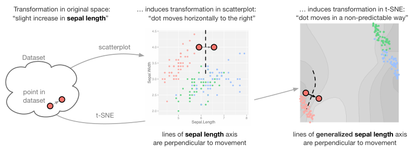
Consider van der Maaten and Hinton’s t-SNE, arguably the most powerful and currently most popular method for NDR [35]. Although practical experience attests to t-SNE’s power to uncover cluster relationships in very challenging datasets, its sensitivity to the hyper-parameters is remarkable [52]. If small changes in parameter settings produce plots that are fundamentally different, we must ask ourselves: are some results generated by NDR methods just bad? Do different parameter settings show different features of the data? More importantly, how do we even answer these questions?
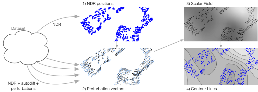
In this work, we design data transformations, which induce transformations on the visualization itself, elucidating the behavior of the NDR method (this is the perspective introduced by Kindlmann and Scheidegger’s algebraic design process [31]). Specifically, we use infinitesimal perturbations — small changes of the data in its original space — to produce infinitesimal changes of the visualization. We then show how these visualization changes can be interpreted as producing effective, non-linear axis legends. In this way, our non-linear axes explain the NDR plot in the same way that axis legends explain the positional encoding in scatterplots. As a result, analysts can understand and evaluate dimensionality reduction plots similarly to how they evaluate linear methods. In fact, we show in Section 3 that our methods exactly recovers the gridlines of typical scatterplots. DimReader is quite general, and can be applied to many different NDR techniques, only requiring access to the source code of its implementation. Specifically, we use a method known as automatic differentiation to produce the necessary gradients for calculating the infinitesimal changes of the visualization [26]. An overview of the process is given in Figure 2.
In summary, our contributions are:
- •
A general framework to explain plots generated by non-linear dimensionality reduction, using infinitesimal perturbations
- •
A practical implementation of the framework using automatic differentiation
- •
A method for discovering good perturbations for a given dataset, useful when the input lacks easily interpretable dimensions (and hence, lacks easily-defined perturbations)
- •
2 Related Work
Projection methods have received a considerable amount of attention in information visualization. In this section, we review the work that is most directly related to our research, but cannot hope to cover the entirety of the field. For a comprehensive view on multidimensional scaling and dimensionality reduction, we recommend Born and Grönen’s textbook [5], and Fodor’s survey [23].
Projection methods in information visualization
The observation that pairwise similarities (or distances) can be converted into low-dimensional representations by a mathematical formulation comes from Torgerson and his now-classical theory of multidimensional scaling [48]. In information visualization, force-directed methods have long been used as a dimensionality reduction technique, from fully-automatic methods [12, 36, 28], to methods which take some amount of interaction, either through placement of exemplar points [37, 30, 21] or through direct interaction with projection parameters [29]. Although interactive methods offer a better hope for understandability because the perturbation analysis we discuss can happen “in the analyst’s head” during interaction, we argue that the visual encoding these techniques provide can still be unclear. The technique we propose here can be applied to essentially all of the methods above, and offers an attractive complement to both automated and interactive projection methods.
Perturbation Analysis for data science
The idea of understanding a system by examining its behavior under perturbations is well-established in the engineering and statistics literature. In the 1970’s, Cook introduced the notion we now know as Cook’s distance [17], which measures the influence of a point on the parameters of linear regression models. In the context of visualization, Bergner et al. point to sensitivity analysis as one of the requirements in understanding computer simulations [4]. In this paper, we use perturbation analysis as a central tool to recover readable axes from NDR methods, in a sense incorporating sensitivity analyses into familiar visual metaphors.
Automatic Differentiation
Perturbation analysis is clearly an important tool for understanding systems, but the issue of how to implement it in existing computer systems is crucial. Automatic differentiation (which we explain in detail in Section 3) provides a way to compute derivatives of arbitrary functions in a computer program, provided access to the source code (or similar structural information about the computation) is available [26]. To the best of our knowledge, the most mature software library employing automatic differentiation is Ceres, written in C++ and employing template metaprogramming [1]. DimReader is implemented in Python for simplicity and terseness, but could easily be redesigned in C++.
Guidance and validation of projection results
One of the issues with NDR is that it’s hard to know what a plot is actually showing[50]. This has resulted in a variety of papers which offer guidance and design principles on how to interpret projections, based on a combination of real-world experience, synthetic examples, and theoretical arguments [9, 42, 43, 40, 33]. This work is essential to the current practice, we argue, because current NDR methods do not offer explanations of their own results — there are much fewer research papers offering guidance for understanding and interpreting traditional scatterplots. As we show in Section 4, our technique provides a way for a projection method to explain itself. Although analyst guidance and validation will always be a part of a well-designed analysis infrastructure, our technique could mitigate some of the problems that have been observed in deployed systems, where projection methods are ultimately discarded because of readability issues [7, 27].
Augmented visual representations
There is another avenue of attack on the readability problem of NDR methods. Often, researchers will augment the results of the projections with visual diagnostics that pinpoint potential problems. Seifert et al. augment the projection by showing how the projection’s stress (roughly the discrepancy between source-space distances and target-space distances) varies spatially in the NDR plot [44]. In [3] and [34], the projection is augmented to show uncertainty measures and distortions in NDR’s respectively. Cutura et. al’s VisCoDeR allows users to compare and explore different dimensionality reductions by augmenting the projection to allow users to explore how dimensions are mapped in the dimensionality reduction results as well as the high-dimensional proximity of projected points to a selected point in the projection [19]. Stahnke and co-authors described methods to probe a projection, through carefully designed user interactions and custom visual encodings [46]. Our method for extracting effective axes can be seen as a way to allow any NDR method to augment itself with metaphors that have a well-defined analogy in the linear case, as can be seen in Section 4, and Figure 7 specifically. In Section 4.3, we provide a more direct comparison to some of the methods used in Stahnke et al.’s work.
Explainable visualizations
Every plot assumes an audience that can read it, and visualization literacy remains an active area of research [6]. Often, novel metaphors are necessary because of the data or task complexity [8]. We argue that generalizing well-established techniques such as axis legends to NDR can help explain those techniques. Gleicher’s Explainers take user interaction to design specific projections for input data [24]. In contrast, our technique extracts axes inherent in the non-linear projections. Coimbra et al. explain projections through enhanced biplots [16]. Similar to our technique, they show axes for the dimensions of the input data in the low dimensional plot. Because of the non-linearity of these dimensionality reductions, the biplot axis will change based on the projected position of the sampled point whereas our technique captures the axis lines for the entire projection. A similar approach is proposed by Cavallo and Demiralp in Prolines, a technique for interacting with data points in both low- and high-dimensional spaces [11]. Prolines allow efficient, direct manipulation of the output points, but require access to efficient forward and backward projection, limits its applicability. Flow-based scatterplots [13] and Generalized Sensitivity Scatterplots [14] show the sensitivity of a dimension in a scatterplot with respect to other dimensions in the dataset. Similar to our technique, these methods use derivatives to determine the sensitivities. Our technique differs by showing sensitivity of the projection with respect to the original data rather than sensitivity between dimensions in the original data. The data context map from Cheng et. al. provides a way to simultaneously look at clusters of data points and the location of the most dominant values of each attribute with the assumption that the attribute values always decrease as points move farther away from it. [15]. Our technique differs by showing the behavior of a dimension throughout the entire projection, not just the location of the most dominant value.
3 Technique
Our technique is broken into two parts: (1) explaining an NDR method using a known perturbation (DimReader ) and (2) searching for good perturbations when there is no known perturbation (after which DimReader can be applied).
In principle, all that DimReader requires is the ability to compute derivatives of the projection coordinates with respect to each of the input points. For extremely simple techniques (such as scatterplots and other fixed linear projections), these derivatives can easily be evaluated in closed form. However, more sophisticated methods such as Isomap, LLE, and t-SNE involve long computation chains, for which the evaluation of the derivative would introduce significant development overhead. Instead of trying to solve them in closed form, we take central advantage of automatic differentiation. [26]. As we describe next, automatic differentiation allows us to calculate the derivative of a projection with minimal implementation effort.
3.1 Automatic Differentiation
In this paper, we use a particular form of automatic differentiation known as forward-mode automatic differentiation. In what follows, we will refer to it as “autodiff”.
In forward-mode autodiff, the program’s derivative with respect to a specified variable is computed alongside the function value, by using an extended number system. In this system, we replace numbers in the program with dual numbers that have the form where holds the original value of the number and carries the derivative of with respect to our variable of interest. When we initialize a variable , we set to one if that is the variable we want to differentiate with respect to (since ) and zero otherwise. When the projection is run with dual numbers in place of regular numbers, in addition to calculating the projected points, it calculates their derivatives through applications of the chain rule and derivative rules (product rule, quotient rule, etc.).
Note that autodiff is always performed at a specific value, and with respect to a specific variable. It produces two numbers as a result: the function value and the partial derivative with respect to the chosen variable. This has two important consequences for our design. First, we need to decide over exactly which variables we will take derivatives. Second, we need to execute the program many times in order to evaluate many different derivatives. This will become important in Section 4.4.
3.2 DimReader Process
3.2.1 Overview of the process
To apply DimReader to an NDR method, there are four steps. Each of these steps is discussed in a subsection below.
- •
A user chooses a perturbation of interest, which defines an infinitesimal change for each data point (possibly in different directions).
- •
The NDR method is executed many times using dual numbers, from which we obtain the perturbation vectors, one for each input point.
- •
From the perturbation vectors, a scalar field whose gradient matches the perturbation vectors is computed.
- •
The isolines of this scalar field, which are perpendicular to the gradient, are extracted using Marching Squares. They form the effective axes.
3.2.2 Choosing which perturbation to use
The first step of our method involves a choice of the perturbation of the dataset. A perturbation is a small change to a specific dimension (or set of dimensions) for each data point in the original, high-dimensional space. Thus, the choice of perturbation corresponds, effectively, to an analyst answering the following question: “if each data point were slightly different in this specific way, what would happen to the visualization?” In order to recover different features of the NDR method and its effect on the dataset of interest, different perturbations can be designed. In the following, we discuss choosing a perturbation in a dataset with interpretable dimensions. We discuss discovering perturbations for other datasets in Section 3.4. In automatic differentiation, perturbations are represented by the derivative part of the dual number for the original data points. The perturbation of a data point with dimensions has the form of a unit vector with elements where the value of each element specifies how much the corresponding dimension is perturbed relative to the rest of the dimensions.
Datasets with interpretable dimensions
Some datasets have interpretable columns. Take the iris dataset, for example, which is used in Figure 2. In that case, a perturbation that changes each of the input points in the direction of a given dimension will reconstruct, for an NDR method, curved axes lines that correspond, roughly to the linear grid lines in scatterplots. Concretely speaking, we evaluate each input point as , where the value is positioned at the dimension of interest.
3.2.3 Extracting derivatives from NDR methods
In this section, we describe two techniques used in DimReader to extract the perturbation vectors ,the changes to the projected coordinates resulting from a perturbation on the input, for a given projection. The first technique is simple, straightforward, and provides a good intuition for the overall strategy. Unfortunately, this technique requires as many executions of the NDR method as there are input points in the dataset, which often means the overall performance can suffer. The second technique, on the other hand, only requires as many runs as the logarithm of the number of input points. We give pseudo-code for the two approaches in Figure 4.
DimReader needs access to the source code for the NDR method at this step so the method can be executed with dual numbers. In principle, the source code can be executed without any modifications aside from converting the input points into dual numbers. In practice, some issues arise because of efficiency concerns and library limitations. We discuss these issues at length in Section 4.

Perturbing one point at a time
After a perturbation is chosen, the NDR technique is executed with automatic differentiation for every point in the dataset. On execution , the point is perturbed (that is, we replace with where is the specified perturbation of ). The NDR technique will return the projection coordinates, , for all points, along with the derivative of the projection coordinates with respect to the perturbation of , . We use the derivative of each coordinate in the reduced point as the vector that describes the change in the coordinate, and discard the rest of the information of the run. The pseudocode for this is given on the top half of Figure 4.
Perturbing many points at a time
The method described above is inefficient, requiring evaluations of the NDR method. A naive attempt to optimize the method would evaluate the projection derivatives with respect to all of the points (and hence all of the per-point perturbations) at once, and only run the autodiff version of the code once. Unfortunately, this does not work for many perturbations, because most DR methods are invariant to dataset translations. The perturbation of only one input point at a time offers interesting insight into the NDR method, but if we move all of the points at once in the same direction, NDR methods such as Isomap, LLE, and t-SNE will produce exactly the same projection (the perturbation vectors will be all zeros).
We solve this problem by adding a small amount of randomization. Instead of perturbing one point at a time, we can choose half of the points at random to perturb, while the other half does not change. We then store the projection vectors for the points we chose to perturb, and repeat the process until we have actually perturbed all of the input points. After each round, we expect to halve the number of unperturbed points, which gives an expected number of repeated runs which is logarithmic on the number of input points. The pseudocode for this is given on the bottom half of Figure 4. We found that the DimReader plots produced by perturbing many points at a time are indistinguishable from the plots produced by perturbing one point at a time.
Ignoring changes in unperturbed points
In some cases, perturbing a point has an effect on points other than its corresponding projected point . However, the effects on other points are small enough that we can effectively ignore them. In Figure 5, we show that the effect of perturbing each point on the other points, () tends to be near zero and very rarely is significant. We show this result for the iris dataset, but have found it to be true in general for t-SNE in all datasets we checked. Intuitively, we expect a good dimensionality reduction to be robust to a small change in a single point, and thus the residual effect on the rest of the points to be insignificant.
3.2.4 Reconstructing the direction field
Once we have the projected points and their derivatives (that is, the perturbation vectors), we need to reconstruct the direction field, in order to extract perpendicular lines. We achieve this by computing a scalar field whose gradient best matches the vectors. We use a simple least-squares reconstruction technique, adapted from Ferreira et al.’s vector-field clustering work [22], which we illustrate in Figure 6. We first decompose the output plane in a rectangular grid, and split each grid square into two triangles, giving a triangular mesh of the output space. The resolution of this grid needs to be decided ahead of time, and we use a 10x10 grid in our examples for this paper. We model a scalar field on the output plane as a piecewise-linear function on the grid values. Each point and its perturbation vector is interpreted as a linear constraint on the vertices of its corresponding triangle. To find the best-fitting scalar field, we solve it in a least-squares sense, regularizing the system to ensure a unique solution [22].

3.2.5 Extracting perpendicular lines
The final step is quite simple. With the scalar field expressed as values in a triangular mesh, we can use marching squares to extract isocontours [2]. By construction, the gradient of this scalar field matches the perturbations. Since isolines are perpendicular to a function’s gradient [41], the resulting curves will tend to be perpendicular to the perturbations. As we show in Figure 2, these isoline can be thought of as generalized axes lines.
3.3 Interpreting DimReader Plots
In our plots, the projected points would move perpendicular to the isolines nearest to them if the input were perturbed in the specified way. An increase in the corresponding dimension would move the point from light to dark. The relative density of the isocontours can be interpreted similarly to the behavior in scalar fields. Narrowly-spaced isocontours indicate a high sensitivity to changes in the independent variable, (in our case, projection coordinates). Widely-spaced isocontours indicate low spatial sensitivity: a change in the projection coordinates is not expected to change the outcome variable by much. Curved isolines indicate that the same perturbation has a different effect on different points. Isolines that fan out (go from narrowly-spaced to widely-spaced as in Figure 8) indicate that the sensitivity of the plot is changing from more sensitive on one side to less sensitive on the other.
3.4 Discovering Good Perturbations
We may not always know good perturbations for a dataset, such as the MNIST digits where it is not clear what the best way to perturb each image would be. To help solve this problem, we offer two methods to recover good perturbations. We define good perturbations as perturbations on the input that change the projection the most under the given constraints. Both of the methods require that we have a tangent map, , for the projection. The tangent map allows for efficient calculation of the perturbation vector, , for a given projection, without running the projection itself. Given a perturbation on the input , results in the perturbation vector , i.e. where is the projected coordinates. The vector consists of the perturbation of each input point concatenated into a single vector (end to end) and the perturbation vector consists of the perturbation vector of each projected point () concatenated into a single vector. A single column of can be recovered by a perturbation vector that has a single entry of 1 and the rest zeros (i.e. perturbing a single dimension of a single point). By doing this for each dimension of every point, the entire tangent map can be recovered.
One observation about the tangent map is that the values we need for calculating the perturbation vectors lie in blocks along the diagonal, where is the dimension of the projection (typically 2) and d is the dimension of the input data. Because we ignore the effect a given perturbation on all other points (as discussed in 3.2.2), we set the rest of the matrix to zero. We exploit the block structure of the tangent map in both of our methods for finding the best perturbation.

3.4.1 Perturb all points in the same direction
The first method for recovering the best perturbation is to find the single perturbation that when applied to all points changes the projection the most. The formulation for this method is:
where is the block on the diagonal of for point i. This can be rewritten as . To find the maximum, we take the derivative with respect to and set it to zero: . The best perturbation vector is the eigenvector of the matrix with the largest eigenvalue. This gives us a single perturbation, , that when applied to all points maximizes the change in the projection. is constrained to have unit length to prevent the method from choosing an arbitrarily large perturbation.
3.4.2 Perturb each point individually
The second method for recovering the best perturbation is to find different perturbations for each point that collectively change the projection the most constrained so that points that are projected to similar places have similar perturbations. The formulation is as follows:
where is the block on the diagonal for point i, is the perturbation for the point i, is a free parameter for how much smoothing we want, and is the similarity between the projection of points i and j, and . This similarity is defined as . is a free parameter set by the user that determines how close points have to be in the projection to be considered similar. We can rewrite the above equation as follows:
We observe that takes form similar to a Laplacian matrix, multiplied by the entire perturbation vector (the concatenation of all of the individual perturbations, ) on both sides: . differs from a standard Laplacian matrix in that rather than having diagonal values and off diagonal values , it has diagonal values and off diagonal values where is identity matrix.
Furthermore, the equation can be rewritten in terms of the whole matrix, , and the entire perturbation vector, giving us the following equation which incorporates the constraint on the length of :
Taking the derivative with respect to and setting it to zero, we get
The entire perturbation vector, , is the eigenvector of the matrix with the largest eigenvalue.
Choosing and .
controls the width of a gaussian centered on each point. Examining the results of the projection itself gives some information about plausible values for . For example, points outside further than three standard deviations from each other are essentially treated independently, but at the same time, we don’t want a that creates a gaussian which covers the entire projection. For choosing , we should be looking at the resulting perturbations. If a single point is heavily dominating the perturbation (i.e. it moves much more than the rest of the points) then is likely too small. In contrast, if all points are perturbed in almost exactly the same way, this is an indication that may be too large.
4 Implementation and Experiments
In this section, we discuss the implementation of our techniques along with a suite of experiments designed to explore the capabilities, performance, and limitations of DimReader. We will show how DimReader directly addresses the following gaps identified in Sedlmair et al.’s interview study about gaps between theory and practice in dimensionality reduction (DR) [42]. These include the interpretation gap: “what do the results mean?”; guidance gap, “what algorithm to use?”, and the non-linear unmapping gap: “how do projection dimensions relate to input dimensions?”.
Our current prototype for DimReader is implemented in Python and numpy [51]. Our t-SNE implementation is closely based on van der Maaten’s Python code [49], while the LLE and Isomap implementations are from-scratch. The entire method takes about 3,500 lines of Python, including implementations of Marching Squares, the classes for autodiff, and the linear solvers described below.
4.1 DimReader
In the following we look at a well known dataset, the iris dataset, with known perturbations, and simple projection algorithms, in order to better understand the behavior of the technique [32].
4.1.1 Linear projections
We start with showing results of linear projections as a basic sanity check on the behavior of DimReader. Figure 7 shows a typical example of the axes reconstructed by DimReader when using linear projections. Since linear projections can be exactly represented by a matrix multiplication, the derivatives of input points position with respect to one direction will always be constant vectors. As a result, the reconstructed scalar field is almost (except for the influence of the regularization terms) a linear ramp, and so the contour lines are evenly spaced and parallel, which indicate that changes in the input variable will behave identically across the entire field. Despite their limited power, this property is one of the main advantages of linear projections.
4.1.2 Isomap
Isomap was one of the first NDR techniques to recover curved manifolds well in practice [47]. Isomap builds a weighted graph which approximates the manifold, where edges have weight equal to the distance between points, and each point has edges to its nearest neighbors ( is specified by the user). The global distance between two points is defined to be the shortest-path metric on the graph. The low-dimensional projection is constructed from the shortest-path metric using classical MDS [5].
We implemented Isomap not only because of its historical significance and relatively high-quality results, but also because it highlights an interesting property of automatic differentiation: it works over code bases that we tend to not think of as differentiable. Specifically, the operations in Dijkstra’s algorithm for shortest paths are all well defined for dual numbers, and so we naturally can extract the sensitivity of shortest-path distances with respect to changes in the input points [18].
Interaction with numerical linear algebra routines
The final step of Isomap is Classical MDS, and this presents unique challenges for our autodiff implementation based on operator overloading. Specifically, Classical MDS requires the computation of eigenvectors, and since Python libraries for numerical linear algebra are implemented through high-performance libraries like Lapack, the operator-overloading functionality is not present. To solve this issue, we implement the eigenvalue computation through power iterations [25], since matrix-vector multiplication of dual numbers has efficient dual-number implementations in terms of matrices of values and terms.
Isomap Experiments
Because Isomap uses classical MDS (which is essentially a linear projection), we should expect that, to some degree, Isomap would behave much like linear projections. This is indeed the case with simpler datasets, such as the Iris dataset, shown in Figure 7. However, there are some interesting differences. Consider the generalized axis for the “sepal width” variable which DimReader recovers. Even though the point positions generated by Isomap are quite similar to that of PCA, the sensitivity of the projection differs dramatically from the cluster of Setosa samples to that of Virginica and Versicolor samples. Even more interestingly, it seems that the sensitivity is caused by only some of the Setosa samples. This differentiation is not present in the linear projection, and would not be clear from the Isomap plot alone. In this example, DimReader helps overcome Sedlmair’s interpretation gap by providing an explanation for why Isomap spread the points in the Setosa cluster (Isomap is sensitive to differences in the Sepal Width in this cluster) that would otherwise be unknown.

4.1.3 Locally Linear Embedding
The next algorithm we highlight is Roweis and Saul’s Locally Linear Embedding [39] (LLE). Like Isomap, LLE uses a nearest-neighbor graph to recover a global view of the dataset. LLE computes edge weights for the nearest neighbor graph, such that each vertex can be best reconstructed by a linear combination of its neighbors using those weights. On a second step, the projection coordinates are recovered by finding positions on the plane that best respect the weights.
Interaction with numerical linear algebra routines
Similarly to Isomap, our autodiff implementation of LLE involves a small degree of adaptation. In the case of Isomap, we required the computation of the largest eigenvalues of a matrix. In the case of LLE, we need to compute the smallest non-zero eigenvalues. Our implementation uses inverse power iteration [25]. Inverse power iteration, in turn, requires a linear system solver, which presents similar issues for dual number implementations. Our solution is to implement a black-box linear system solver using conjugate gradients [45].
LLE Experiments
Locally Linear Embedding is a popular method due to its performance [39], but is known to produce distorted projections [20]. In this section, we illustrate how DimReader might help pinpoint such problems. Consider the projection of the iris dataset in Figure 7. Note that neither of the recovered axes quite cross the projection perpendicularly on the left side of the arc (the Versicolor and Virginica cluster): no direction of perturbation on the input moves the points diagonally along that cluster. This suggests that the shape of the cluster is an artifact of the projection method. Compare this with the Isomap projection in Figure 7: Isomap has perturbations which cross each of the clusters perpendicularly (Sepal Width for Setosa and Sepal Length for Versicolor and Virginica). Thus, Isomap is more faithful to the underlying data than LLE. This is evidence that DimReader helps bridge Sedlmair et. al’s guidance gap [42], giving an indication for which NDR algorithm performs better for this data.
4.1.4 t-SNE
t-SNE is among the most powerful techniques for dimensionality reduction, and also one of the hardest to interpret appropriately [35, 52]. As such, it is a natural target for DimReader. In addition, t-SNE is significantly different from Isomap and LLE in both formulation and implementation. This provides us with an opportunity to explore practical issues of using DimReader to explain its results.
We highlight two separate issues to discuss: the presence of multiple local minima, and its formulation in terms of the gradient of an energy function. While the first issue presents challenges for implementations that depend on repeated executions, the second issue allows us to achieve a significant speedup.
Multiple minima
The energy function that t-SNE minimizes has more than one local minimum. This means that any source of randomness in the implementation will cause multiple runs to possibly diverge, presenting a challenge for our approach. Most implementations of t-SNE require an initial guess for the projection, and we take central advantage of this. Specifically, in our first execution of t-SNE we use a random initial guess and regular floating-point numbers to calculate a local minimum that is then used as the initial guess for subsequent runs. In the initial run we also capture variables that serve as parameters for subsequent runs to ensure that they reach the same local minimum.
Gradient descent
t-SNE is implemented as an explicit gradient descent formulation through an additive update of the parameters. Specifically, the main loop of t-SNE is roughly as follows:
As a result, when the loop exits, we know that the gradient of the energy with respect to the position will be close to zero. This means that to recover any one perturbation of the t-SNE formulation with respect to an input point, all that is required is to run one single iteration of t-SNE with dual numbers. By providing the dual-number implementation the result of the execution of the floating-point implementation (as explained in the previous paragraph), the loop will execute at most once before exiting – in fact, in order for the sensitivity of the positions with respect to the input to be recorded in the pos variable, we must force the loop to execute at least once. Still, since t-SNE typically executes between 100 and 1000 iterations in this loop, this simple optimization achieves a significant speedup.
t-SNE Experiments
T-SNE is often considered to be the state of the art in NDR methods, but one of the main objections to its use in practice is the opaque nature of its optimization criteria [52]. It is unclear how effectively the projection recovers high dimensional information. Consider the t-SNE axes in Figure 7. t-SNE is detecting variation in the petal length and petal width of the Virginica and Versicolor cluster and subsequently spreading the cluster based on these dimensions. This helps explain how petal length behaves in the projection, providing evidence that DimReader helps bridge the non-linear unmapping gap [42].
4.2 Discovering Perturbations
The implementation of the equations in 3.4 for discovering perturbations is straightforward as long as the machine has sufficient memory to hold the expanded laplacian matrix, . This matrix becomes very large for very high-dimensional data and thus requires significant memory. To solve this problem, we were again able to exploit the block structure of the tangent map as well as the structure of the Laplacian matrix: the diagonal values are and the off diagonal values are . We implemented a version of power iteration that does not require access to the matrix but instead requires a function that, when given a vector , returns . The multiplication function calculates elements of the output vector individually and thus does not require the entire matrix.
Using this method, we uncovered perturbations for several datasets projected with t-SNE. In the following experiments, we use the method in Section 3.4.2 to find individual perturbations for each point.
4.2.1 Iris
We first look at the best perturbation for the Iris dataset. Figure 8 shows the DimReader plot for this perturbation as well as a plot for each dimension that shows how much that dimension was perturbed in each point through the color (the darker purple a point is, the more it was perturbed). The DimReader plot shows that the best perturbation only perturbs points in the Setosa (red) cluster. In the individual dimension plots, the Setosa cluster is perturbed primarily in the Sepal length and Sepal width dimensions which tells us that in this projection, points in the Setosa cluster are sensitive to changes in the Sepal dimensions. Comparing 8 to the t-SNE plots in Figure 7, the movement of the Setosa cluster with the discovered perturbation is similar to the movement when the sepal width or sepal length is perturbed.
4.2.2 MNIST Digits
Figure 9 (A) shows an sample of discovered perturbations in the projection. The perturbation images often resemble a variation of their corresponding digit or a nearby digit (due to the constraints defined in Section 3.4.2). These perturbations show us that t-SNE is capturing meaningful information about the dataset. In Figure 9 (A), the perturbation that moves the ”seven” the most turns the ”seven” into a “two” and moves it toward the cluster of “two”s. Thus, DimReader, is showing evidence that t-SNE is capturing information about what constitutes a “two” and is using that information to separate out the two’s into their own (imperfect) cluster.

4.2.3 MNIST Fashion
The MNIST Fashion dataset is similar to the digits dataset in that each point represents a pixel image and there are 10 different classes of images (articles of clothing) but is more complicated than the digits dataset. A t-SNE plot with selected perturbations found by our technique is shown in Figure 9 (B). Just as in the digits perturbations, there is structure in these perturbations. In the example in Figure 1 (C), our technique is finding perturbations that capture information about how t-SNE is projecting the data. DimReadertells us, that for the heel in the middle, the perturbation that moves this point the most, changes it from a heel into a flat shoe. This also shows us that t-SNE understand the difference between flat shoes and heels and is able to separate them.
4.3 Synthetic Examples
In this section we will look at the DimReader plot with two synthetic examples, the swiss roll and the interlocked rings, and compare them to the value heatmaps for each dimension from Stahnke et. al’s Probing Projections.
4.3.1 Swiss Roll
The swiss roll dataset is calculated from the equations , , where and . Figure 10 shows perturbations of the U,V, and X dimensions.

PCA
In the dimension, the DimReader plot shows that increasing the in the original data moves the projected points to the left. In comparison, the value heatmap for the dimension is difficult to read due to the high variance in between neighboring points. This highlights a fundamental difference between DimReader and value heatmaps: DimReader is showing what the projection is doing while value heatmaps show the values of a dimension based on the placement of points. If we created a projection that simply mapped each point to its PCA coordinates through a table lookup, the value heatmaps would not change whereas the DimReader plots would show nothing because changing any of the dimensions would not change the projection.
The DimReader plot for the dimension shows that changing the dimension would move the point along the spiral, from red to blue. The isolines, however, are irregular from green to orange. These irregularities could be due to the resolution of the grid or the regularization. One direction for future work is to automatically determine the appropriate grid resolution and regularization for a projection.
t-SNE
In the DimReader plot for t-SNE, the dimension behaves exactly as we would expect, increasing as we move from red to blue. The spacing of the lines around the curve, specifically how the curves are wider on the outside than on the inside, indicates the bending does not reflect the underlying data but rather is caused by the projection.
In the DimReader plot for , t-SNE has flipped the green and yellow segment (the points move to the bottom left rather than the upper right). This appears less clear from the value heatmap alone.
In the plots for , the highest values in the heatmap do not match the area in the DimReader plot where the biggest change occurs.
4.3.2 Interlocked Rings
The DimReader plots and value heatmaps generated for the interlocked rings dataset are shown in Figure 11.
PCA
The PCA plots from DimReader show that changing X or Z would move the points upward and changing the Y dimension move points to the right. Again, the plots here highlight the difference between our technique and the value heatmaps: the heatmaps of x and z tell us that the x and z values are only changing over one ring each whereas our technique is showing that PCA will move the rings vertically if the x or z dimension is changed. DimReader shows what the projection does, whereas heatmaps shows where the values go.
t-SNE
T-SNE has separated the two rings well. In the DimReader plot of the X dimension, the red ring will move from left to right when the X dimension is changed. Comparing the X dimension to the Y dimension, for the red ring, the two axes are nearly perpendicular to one another. This suggests that t-SNE is primarily using these two dimensions for projecting the red ring. Furthermore, in the red ring the X dimension changes much quicker than the Y dimension (the lines are closer together) which indicates that t-SNE is distorting the shape of the red ring. Similar observations can be made about the green ring with the Y and Z dimensions. Again, the Y and Z are nearly perpendicular in the green ring. In the Y dimension, the axes change their behavior when they reach the gap in the green ring. Points in this region move more slowly when changed which in turn tells us that this is likely a tear in the ring caused by t-SNE that does not reflect the structure of the underlying data. It is not as clear from the value heatmaps that the gap is a tear in the data caused by the projection.
4.4 Performance
4.4.1 Known Perturbations
In this section, we report performance figures for the prototype implementation of DimReader. Although we were reasonably careful with algorithmic and high-level design decisions that impact performance, we did not make a significant effort to make DimReader fast. We expect carefully-implemented versions of our proposal in high-performance languages such as C++ or Java to be significantly faster, possibly by an order of magnitude (typically the performance difference between Python and aggressively optimized, compiled languages).
A table showcasing typical results is included in Figure 12. The performance of DimReader for a given NDR method is dependent on two main factors: the number of input points and the overhead incurred by dual numbers. We need to execute a number of repeated runs proportional to the base-2 logarithm of the number of input points, and that is essentially unavoidable. We note that for the case of LLE and t-SNE, the optimizations we described in the previous section make the execution of the dual-number version of the projection much faster than that of the regular numbers. As a result, DimReader can extract axes with a relatively small performance overhead.
For cases such as Isomap, on the other hand, where we performed no such optimizations, the performance of our method suffers a bit. We argue that this is an acceptable tradeoff: DimReader still works in an acceptable amount of time in the general case, but more careful implementations can be significantly more efficient.
4.4.2 Discovering Perturbations
The most expensive part of searching for a perturbation is calculating the tangent map. The tangent map is and requires executions of DimReader to build it. For datasets with a large number of data points and dimensions, this quickly becomes slow. Once we have the matrix, the performance for finding the best perturbation largely depends on whether or not we can the expanded Laplacian matrix, , (described in Section 4.2) in memory. If we can’t and have to use power iteration, the performance depends on the speed of our multiplication function as well as the amount of time it takes power iteration to converge. We did not make a significant effort to increase the performance for calculating the matrix or searching for perturbations; this remains for future work.
5 Discussion
Can we trust DimReader plots?
While we have shown that DimReader can help determining how NDR plots can be trusted, a natural question to ask is: can the DimReader plots themselves be trusted? One natural scenario in which this comes up is when perturbation vectors of nearby projections disagree with one another. It’s always possible to show the vectors themselves as a diagnostic of the quality of the reconstructed axis lines, but a proper, user-centric evaluation of the settings in which DimReader’s axes are more informative than naked NDR plots is clearly necessary, and will be the subject of future work.
Inverse readings
DimReader enables interpretation of forward transformations: given a perturbation of an input and a visualization, DimReader provides an answer. But a different natural reading is the inverse: given a projected point and a direction of movement in the projection, what changes in the data could generate such movement? In principle, the derivative information obtained by autodiff also captures this inverse relationship [10], but the fact that we are dealing with projections makes the problem fundamentally harder. A full investigation is beyond the scope of this work.
More algorithms, better infrastructure
While DimReader shows that it is possible to adapt a large number of existing NDR methods to run within an autodiff framework, one goal is to provide DimReader axes to as much existing visualization infrastructure as practically possible. In such scenarios, reducing the implementation effort even further would be desirable. The majority of our difficulties porting algorithms to automatic differentiation arose due to difficulties in evaluating derivatives of linear-algebraic concepts, such as solutions of a linear system and eigenvectors. Some of these have explicit formulas [38], but incorporating them in an autodiff system effectively and efficiently is a fundamental challenge beyond the scope of our work. We note, in addition, that our choice of automatic differentiation is not strictly necessary. Other methods exist to evaluate function derivatives, including manual derivation of the expressions. When using DimReader with a specific NDR method, these alternatives might be more attractive. This might be particularly true whenever approximations of the derivative can be computed more efficiently than autodiff.
6 Conclusion
In this paper, we identified infinitesimal perturbations as a tool to enable interpretation of NDR plots, and presented DimReader, a technique that produces generalized axes for studying such perturbations. While much work remains to be done, DimReader strikes a favorable balance between generality and power, highlighting strengths and weaknesses of a variety of NDR methods, and providing a novel perspective into what NDR methods are actually visualizing.
Acknowledgements
We acknowledge fruitful discussions of dimensionality reduction with Sean Stephens, Luiz Gustavo Nonato, and Joshua Levine on the energy formulation of t-SNE. This work has been partially supported by the NSF under the TRIPODS program, award number CCF-1740858, and IIS-1513651.
References
- [1] S. Agarwal, K. Mierle, and Others. Ceres solver. \urlhttp://ceres-solver.org.
- [2] E. Angel. Interactive computer graphics: A top-down approach using OpenGL, 2003.
- [3] M. Aupetit. Visualizing distortions and recovering topology in continuous projection techniques. Neurocomputing, 70(7-9):1304–1330, 2007.
- [4] S. Bergner, M. Sedlmair, T. Moller, S. N. Abdolyousefi, and A. Saad. Paraglide: Interactive parameter space partitioning for computer simulations. IEEE Transactions on Visualization and Computer Graphics, 19(9):1499–1512, 2013.
- [5] I. Borg and P. J. Groenen. Modern multidimensional scaling: Theory and applications. Springer Science & Business Media, 2005.
- [6] J. Boy, R. A. Rensink, E. Bertini, and J.-D. Fekete. A principled way of assessing visualization literacy. IEEE Transactions on Visualization and Computer Graphics, 20(12):1963–1972, 2014.
- [7] M. Brehmer, S. Ingram, J. Stray, and T. Munzner. Overview: The design, adoption, and analysis of a visual document mining tool for investigative journalists. IEEE Transactions on Visualization and Computer Graphics, 20(12):2271–2280, 2014.
- [8] M. Brehmer and T. Munzner. A multi-level typology of abstract visualization tasks. IEEE Transactions on Visualization and Computer Graphics, 19(12):2376–2385, 2013.
- [9] A. Buja and D. F. Swayne. Visualization methodology for multidimensional scaling. Journal of Classification, 19(1):7–43, 2002.
- [10] M. P. Carmo. Differential geometry of surfaces. Differential Forms and Applications, pp. 77–98, 1994.
- [11] M. Cavallo and Ç. Demiralp. A visual interaction framework for dimensionality reduction based data exploration. ACM Human Factors in Computing Systems (CHI), 2018.
- [12] M. Chalmers. A linear iteration time layout algorithm for visualising high-dimensional data. In Proceedings of the 7th conference on Visualization’96, pp. 127–ff. IEEE Computer Society Press, 1996.
- [13] Y.-H. Chan, C. D. Correa, and K.-L. Ma. Flow-based scatterplots for sensitivity analysis. In Visual Analytics Science and Technology (VAST), 2010 IEEE Symposium on, pp. 43–50. IEEE, 2010.
- [14] Y.-H. Chan, C. D. Correa, and K.-L. Ma. The generalized sensitivity scatterplot. IEEE transactions on visualization and computer graphics, 19(10):1768–1781, 2013.
- [15] S. Cheng and K. Mueller. The data context map: Fusing data and attributes into a unified display. IEEE transactions on visualization and computer graphics, 22(1):121–130, 2016.
- [16] D. B. Coimbra, R. M. Martins, T. T. Neves, A. C. Telea, and F. V. Paulovich. Explaining three-dimensional dimensionality reduction plots. Information Visualization, 15(2):154–172, 2016.
- [17] R. D. Cook. Detection of influential observation in linear regression. Technometrics, 19(1):15–18, 1977.
- [18] T. H. Cormen. Introduction to algorithms. MIT press, 2009.
- [19] R. Cutura, S. Holzer, M. Aupetit, and M. Sedlmair. Viscoder: A tool for visually comparing dimensionality reduction algorithms.
- [20] D. L. Donoho and C. Grimes. Hessian eigenmaps: Locally linear embedding techniques for high-dimensional data. Proceedings of the National Academy of Sciences, 100(10):5591–5596, 2003.
- [21] A. Endert, C. Han, D. Maiti, L. House, and C. North. Observation-level interaction with statistical models for visual analytics. In Visual Analytics Science and Technology (VAST), 2011 IEEE Conference on, pp. 121–130. IEEE, 2011.
- [22] N. Ferreira, J. T. Klosowski, C. E. Scheidegger, and C. T. Silva. Vector field k-means: Clustering trajectories by fitting multiple vector fields. Computer Graphics Forum, 32(3pt2):201–210, 2013.
- [23] I. K. Fodor. A survey of dimension reduction techniques. Center for Applied Scientific Computing, Lawrence Livermore National Laboratory, 9:1–18, 2002.
- [24] M. Gleicher. Explainers: Expert explorations with crafted projections. IEEE Transactions on Visualization and Computer Graphics, 19(12):2042–2051, 2013.
- [25] G. H. Golub and C. F. Van Loan. Matrix computations, vol. 3. JHU Press, 2012.
- [26] A. Griewank and A. Walther. Evaluating derivatives: principles and techniques of algorithmic differentiation. SIAM, 2008.
- [27] S. Ingram. Personal communication, 2017.
- [28] S. Ingram, T. Munzner, and M. Olano. Glimmer: Multilevel mds on the gpu. IEEE Transactions on Visualization and Computer Graphics, 15(2):249–261, 2009.
- [29] D. H. Jeong, C. Ziemkiewicz, B. Fisher, W. Ribarsky, and R. Chang. ipca: An interactive system for pca-based visual analytics. Computer Graphics Forum, 28(3):767–774, 2009.
- [30] P. Joia, D. Coimbra, J. A. Cuminato, F. V. Paulovich, and L. G. Nonato. Local affine multidimensional projection. IEEE Transactions on Visualization and Computer Graphics, 17(12):2563–2571, 2011.
- [31] G. Kindlmann and C. Scheidegger. An algebraic process for visualization design. IEEE Transactions on Visualization and Computer Graphics, 20(12):2181–2190, 2014.
- [32] R. M. Kirby and C. T. Silva. The need for verifiable visualization. IEEE Computer Graphics and Applications, 28(5), 2008.
- [33] J. Lee and M. Verleysen. Quality assessment of nonlinear dimensionality reduction based on k-ary neighborhoods. In New Challenges for Feature Selection in Data Mining and Knowledge Discovery, pp. 21–35, 2008.
- [34] S. Lespinats and M. Aupetit. Checkviz: Sanity check and topological clues for linear and non-linear mappings. In Computer Graphics Forum, vol. 30, pp. 113–125. Wiley Online Library, 2011.
- [35] L. v. d. Maaten and G. Hinton. Visualizing data using t-sne. Journal of Machine Learning Research, 9(Nov):2579–2605, 2008.
- [36] A. Morrison, G. Ross, and M. Chalmers. A hybrid layout algorithm for sub-quadratic multidimensional scaling. In Information Visualization, 2002. INFOVIS 2002. IEEE Symposium on, pp. 152–158. IEEE, 2002.
- [37] F. V. Paulovich, L. G. Nonato, R. Minghim, and H. Levkowitz. Least square projection: A fast high-precision multidimensional projection technique and its application to document mapping. IEEE Transactions on Visualization and Computer Graphics, 14(3):564–575, 2008.
- [38] K. B. Petersen, M. S. Pedersen, et al. The matrix cookbook. Technical University of Denmark, 7:15, 2008.
- [39] S. T. Roweis and L. K. Saul. Nonlinear dimensionality reduction by locally linear embedding. science, 290(5500):2323–2326, 2000.
- [40] D. Sacha, L. Zhang, M. Sedlmair, J. A. Lee, J. Peltonen, D. Weiskopf, S. C. North, and D. A. Keim. Visual interaction with dimensionality reduction: A structured literature analysis. IEEE Transactions on Visualization and Computer Graphics, 23(1):241–250, 2017.
- [41] H. M. Schey. Div, grad, curl, and all that. Norton, 1973.
- [42] M. Sedlmair, M. Brehmer, S. Ingram, and T. Munzner. Dimensionality reduction in the wild: Gaps and guidance. Dept. Comput. Sci., Univ. British Columbia, Vancouver, BC, Canada, Tech. Rep. TR-2012-03, 2012.
- [43] M. Sedlmair, T. Munzner, and M. Tory. Empirical guidance on scatterplot and dimension reduction technique choices. IEEE Transactions on Visualization and Computer Graphics, 19(12):2634–2643, 2013.
- [44] C. Seifert, V. Sabol, and W. Kienreich. Stress maps: analysing local phenomena in dimensionality reduction based visualisations. In IEEE Int. symposium on Visual Analytics Science and Technology., 2010.
- [45] J. R. Shewchuk. An introduction to the conjugate gradient method without the agonizing pain. Technical report, Carnegie-Mellon University. Department of Computer Science, 1994.
- [46] J. Stahnke, M. Dörk, B. Müller, and A. Thom. Probing projections: Interaction techniques for interpreting arrangements and errors of dimensionality reductions. IEEE Transactions on Visualization and Computer Graphics, 22(1):629–638, 2016.
- [47] J. B. Tenenbaum, V. De Silva, and J. C. Langford. A global geometric framework for nonlinear dimensionality reduction. science, 290(5500):2319–2323, 2000.
- [48] W. S. Torgerson. Multidimensional scaling of similarity. Psychometrika, 30(4):379–393, 1965.
- [49] L. van der Maaten. A Python implementation of t-SNE. \urlhttps://lvdmaaten.github.io/tsne/.
- [50] A. Vellido, J. D. Martín-Guerrero, and P. J. Lisboa. Making machine learning models interpretable. In ESANN, vol. 12, pp. 163–172. Citeseer, 2012.
- [51] S. v. d. Walt, S. C. Colbert, and G. Varoquaux. The numpy array: a structure for efficient numerical computation. Computing in Science & Engineering, 13(2):22–30, 2011.
- [52] M. Wattenberg, F. Viégas, and I. Johnson. How to use t-sne effectively. Distill, 2016. http://distill.pub/2016/misread-tsne.