VIDOSAT: High-dimensional Sparsifying Transform Learning for Online Video Denoising

Denoising is one of the most important problems in video processing. The ubiquitous use of relatively low-quality smart phone cameras has also led to the increasing importance of video denoising. Recovering high-quality video from noisy footage also improves robustness in high-level vision tasks [3, 4].

Though image denoising algorithms, such as the popular BM3D method [5] can be applied to each video frame independently, most of the video denoising techniques (or more generally, methods for reconstructing dynamic data from measurements [6, 7]) exploit the spatio-temporal correlation in dynamic image sequences. Natural videos have local structures that are sparse or compressible in some transform domain, or in certain dictionaries, e.g., discrete cosince transform (DCT) [8] and wavelets [9]. Prior works exploited this fact and proposed video (or high-dimensional data) denoising algorithms based on adaptive sparse approximation [10] or Wiener filtering [11]. Videos also typically involve various kinds of motion or dynamics in the scene, e.g., moving objects or humans, rotations, etc. Recent state-of-the-art video and image denoising algorithms utilize block matching (BM) to group local patches over space and time (to account for motion), and apply denoising jointly for such matched data [5, 11, 12]. Table I summarizes the key attributes of the popular and related video denoised methods, as well as the proposed methods.

Many of the aforementioned video denoising methods exploit sparsity in a fixed transform domain (e.g., DCT) as part of their framework. Several recent works have shown that the data-driven adaptation of sparse signal models (e.g., based on training signals, or directly from corrupted measurements) usually leads to high quality results (e.g., compared to fixed or analytical models) in many applications [13, 14, 15, 16, 17, 18, 19, 20, 21, 22, 23, 24]. Synthesis dictionary learning is the best-known adaptive sparse representation technique [25, 13]. However, obtaining optimal sparse representations of signals in synthesis dictionary models, known as synthesis sparse coding, is NP-hard (Non-deterministic Polynomial-time hard) in general. The commonly used approximate sparse coding algorithms [26, 27, 28, 29] typically still involve relatively expensive computations for large-scale problems.

As an alternative, the sparsifying transform model suggests that the signal $\mathbf{u}$ is approximately sparsifiable using a transform $\mathbf{W}\in\mathbb{R}^{m\times n}$, i.e., $\mathbf{Wu=x+e}$, with $\mathbf{x}\in\mathbb{R}^{m}$ a sparse vector called the sparse code and $\mathbf{e}$ a modeling error term in the transform domain. A key advantage of this model over the synthesis dictionary model, is that for a given transform $\mathbf{W}$, the optimal sparse code $\mathbf{x}$ of sparsity level $s$ minimizing the modeling error $\|\mathbf{e}\|_{2}$ is obtained exactly and cheaply by simple thresholding of $\mathbf{W}\mathbf{u}$ to its $s$ largest magnitude components. Another advantage is that with $\mathbf{u}$ being given data, the transform model does not involve a product between $\mathbf{W}$ and unknown data, so learning algorithms for $\mathbf{W}$ can be simpler and more reliable. Recent works proposed learning sparsifying transforms [19, 30] with cheap algorithms that alternate between updating the sparse approximations of training signals in a transform domain using simple thresholding-based transform sparse coding, and efficiently updating the sparsifying transform. Various properties have been found to be useful for learned transforms such as double sparsity [20], union-of-transforms [21], rotation and flip invariance [31], etc. Transform learning-based techniques have been shown to be useful in various applications such as sparse data representations, image denoising, inpainting, segmentation, magnetic resonance imaging (MRI), and computed tomography (CT) [21, 32, 31, 33, 34, 35, 36, 24, 37, 38].

In prior works on batch transform learning [19, 30, 21, 31], the transform was adapted using all the training data, which is efficient and comes with a convergence guarantee. When processing large-scale streaming data, it is also important to compute results online, or sequentially over time. Our recent work [39, 40] proposed online transform learning, which sequentially adapts the sparsifying transform and transform-sparse coefficients for sequentially processed signals. This approach involves cheap computation and limited memory requirement. Compared to popular techniques for online synthesis dictionary learning [41], the online adaptation of sparsifying transforms allows for cheaper or exact updates [39], and is thus well suited for high-dimensional data applications.

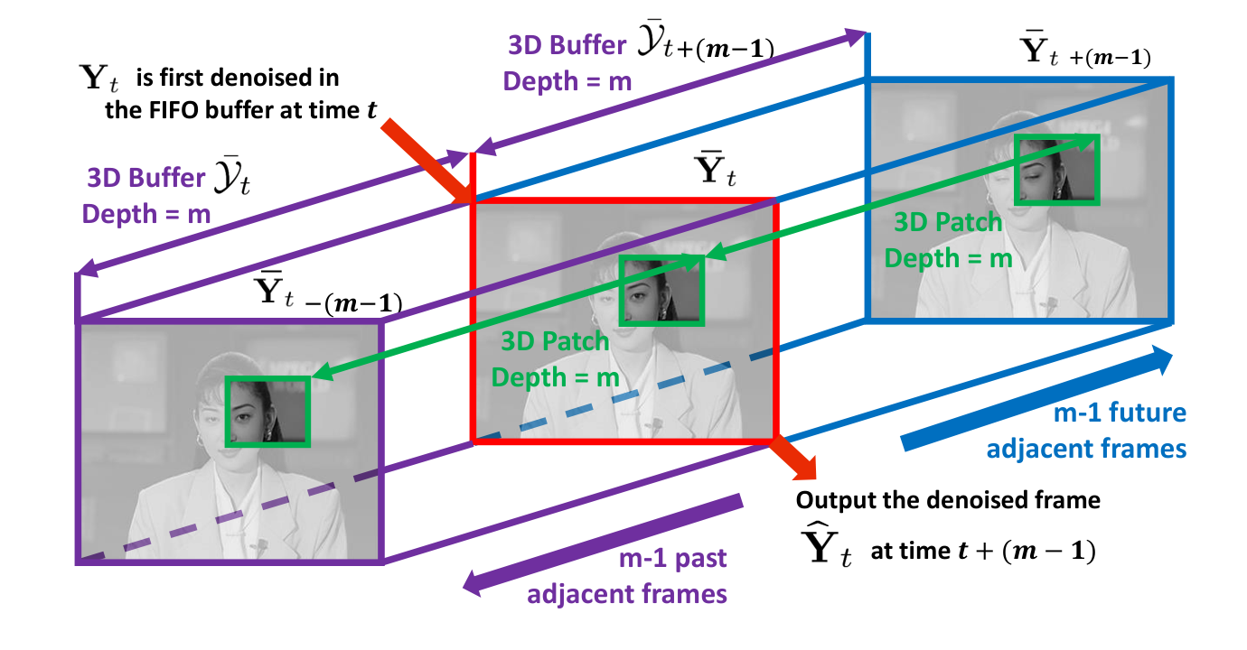
While the data-driven adaptation of synthesis dictionaries for the purpose of denoising image sequences or volumetric data [15, 10] has been studied in some recent papers, the usefulness of learned sparsifying transforms has not been explored in these applications. Video data typically contain correlation along the temporal dimension, which will not be captured by learning sparsifying transforms for the 2D patches of the video frames. We focus on video denoising using high-dimensional online transform learning. We refer to our proposed framework as VIdeo Denoising by Online SpArsifying Transform learning (VIDOSAT). Spatio-temporal (3D) patches are constructed using local 2D patches of the corrupted video, and the sparsifying transform is adapted to these 3D patches on-the-fly. Fig.1 illustrates one way of constructing the (vectorized) spatio-temporal patches or tensors from the streaming video, and Fig.2 is a flow-chart of the proposed VIDOSAT framework. Though we consider 3D spatio-temporal tensors formed by 2D patches for gray-scale video denoising in this work, the proposed denoising methods readily apply to higer-dimensional data (e.g., color video [42], hyperspectral images, dynamic 3D MRI, etc) as well.

As far as we know, this is the first online video denoising method using adaptive sparse signal modeling, and the first application of high-dimensional sparsifying transform learning to spatio-temporal data. Our methodology and results are summarized as follows:

• •

  The proposed video denoising framework processes noisy frames in an online, sequential fashion to produce streaming denoised video frames. The algorithms require limited storage of a few video frames, and modest computation, scaling linearly with the number of pixels per frame. As such, our methods would be able to handle high definition / high rate video enabling real-time output with controlled delay, using modest computational resources.

• •

  The online transform learning technique exploits the spatio-temporal structure of the video tensors (patches) using adaptive 3D transform-domain sparsity to process them sequentially. The denoised tensors are aggregated to reconstruct the streaming video frames.

• •

  We evaluate the video denoising performance of the proposed algorithms for several datasets, and demonstrate their promising performance compared to several prior or related methods.

This paper is an extension of our previous conference work [43] that briefly investigated a specific VIDOSAT method. Compared with this earlier work, here we investigate different VIDOSAT methodologies such as involving block matching (referred to as VIDOSAT-BM). Moreover, we provide detailed experimental results illustrating the properties of the proposed methods and their performance for several datasets, with extensive evaluation and comparison to prior or related methods. We also demonstrate the advantages of VIDOSAT-BM over the VIDOSAT approach of [43].

We use the following notations in this work. Vectors (resp. matrices) are denoted by boldface lowercase (resp. uppercase) letters such as $\mathbf{u}$ (resp. $\mathbf{U}$). We use calligraphic uppercase letters (e.g., $\mathcal{U}$) to denote tensors. We denote the vectorization operator for 3D tensors (i.e., for reshaping a 3D array into a vector) as $\mathrm{vec}(\cdot):\mathbb{R}^{n_{1}\times n_{2}\times m}\rightarrow\mathbb{R}^{n}$. The vectorized tensor is $\mathbf{u}=\mathrm{vec}(\mathcal{U})\in\mathbb{R}^{n}$, with $n=n_{1}n_{2}m$. Correspondingly, the inverse of the vectorization operator $\mathrm{vec}^{-1}(\cdot):\mathbb{R}^{n}\rightarrow\mathbb{R}^{n_{1}\times n_{2}\times m}$ denotes a tensorization operator. The relationship is summarized as follows:

The other major notations of the indices and variables that are used in this work are summarized in Table II. We denote the underlying signal or variable as $\tilde{\mathbf{u}}$, and its noisy measurement (resp. estimate) is denoted as $\mathbf{u}$ (resp. $\hat{\mathbf{u}}$). The other notations used in our algorithms are discussed in later sections.

The rest of the paper is organized as follows. Section II briefly discusses the recently proposed formulations for time-sequential signal denoising based on online and mini-batch sparsifying transform learning [39, 40]. Then, Section III presents the proposed online video processing framework, and two online approaches for denoising dynamic data. Section IV describes efficient algorithms for the proposed formulations. Section V demonstrates the behavior and promise of the proposed algorithms for denoising several datasets. Section VI concludes with proposals for future work.

In prior work [39], we proposed an online signal denoising methodology based on sparsifying transform learning, where the transform is adapted based on sequentially processed data. For time $t=1,2,3$, etc, the problem of updating the adaptive sparsifying transform and sparse code (i.e., the sparse representation in the adaptive transform domain) to account for the new noisy signal $\mathbf{u}_{t}\in\mathbb{R}^{n}$ is

where the $\ell_{0}$ “norm” counts the number of nonzeros in $x_{\tau}$, which is the sparse code of $\mathbf{u}_{\tau}$. Thus $\left\|\mathbf{W}\mathbf{u}_{\tau}-\mathbf{x}_{\tau}\right\|_{2}^{2}$ is the sparsification error (i.e., the modeling error in the transform model) for $\mathbf{u}_{\tau}$ in the transform $\mathbf{W}$. The term $\nu(\mathbf{W})=-\log\,\left|\mathrm{det\,}\mathbf{W}\right|+\left\|\mathbf{W}\right\|_{F}^{2}$ is a transform learning regularizer [19], $\lambda_{\tau}=\lambda_{0}\left\|\mathbf{u}_{\tau}\right\|_{2}^{2}$ with $\lambda_{0}>0$ allows the regularizer term to scale with the first term in the cost, and the weight $\alpha_{\tau}$ is chosen proportional to $\sigma_{\tau}$ (the standard deviation of noise in $\tilde{\mathbf{u}}_{\tau}$). Matrix $\hat{\mathbf{W}}_{t}$ in (P1) is the optimal transform at time $t$, and $\hat{\mathbf{x}}_{t}$ is the optimal sparse code for $\mathbf{u}_{t}$.

Note that at time $t$, only the latest optimal sparse code $\hat{\mathbf{x}}_{t}$ is updated in (P1)¹¹ 1 This is because only the signal $\tilde{\mathbf{u}}_{t}$ is assumed to be stored in memory at time $t$ for the online scheme. along with the transform $\hat{\mathbf{W}}_{t}$. The condition $\mathbf{x}_{\tau}=\hat{\mathbf{x}}_{\tau},\;1\leq\tau\leq t-1$, is therefore assumed. For brevity, we will not explicitly restate this condition (or, its variants) in the formulations in the rest of this paper. Although at each time $t$ the transform is updated based on all the past and present observed data, the online algorithm for (P1) [39] involves efficient operations based on a few matrices of modest size, accumulated sequentially over time.

The regularizer $\nu(\mathbf{W})$ in (P1) prevents trivial solutions and controls the condition number and scaling of the learnt transform [19]. The condition number $\kappa(\mathbf{W})$ is upper bounded by a monotonically increasing function of $\nu(\mathbf{W})$ [19]. In the limit $\lambda_{0}\to\infty$ (and assuming the $\mathbf{u}_{\tau}$, $1\leq\tau\leq t$, are not all zero), the condition number of the optimal transform in (P1) tends to 1. The specific choice of $\lambda_{0}$ (and hence the condition number) depends on the application.

Another useful variation of Problem (P1) involves mini-batch learning, where a block (group), or mini-batch of signals is processed at a time [39]. Assuming a fixed mini-batch size $M$, the $L$th ($L\geq 1$) mini-batch of signals is $\mathbf{U}_{L}=\begin{bmatrix}\mathbf{u}_{LM-M+1}\mid\mathbf{u}_{LM-M+2}\mid&...&\mid\mathbf{u}_{LM}\end{bmatrix}$. For $L=1,2,3$, etc, the mini-batch sparsifying transform learning problem is

where the regularizer weight is $\Lambda_{j}=\lambda_{0}\begin{Vmatrix}\mathbf{U}_{j}\end{Vmatrix}_{F}^{2}$, and the matrix $\mathbf{X}_{L}=\;$ $\begin{bmatrix}\mathbf{x}_{LM-M+1}\mid\mathbf{x}_{LM-M+2}\mid&...&\mid\mathbf{x}_{LM}\end{bmatrix}$ contains the block of sparse codes corresponding to $\mathbf{U}_{L}$.

Since we only consider a finite number of frames or patches in practice (e.g., in the proposed VIDOSAT algorithms), the normalizations by $1/t$ in (P1), $1/C_{t}$ in (1), and $1/LM$ in (P2) correspondingly have no effect on the optimum $\begin{Bmatrix}\hat{\mathbf{W}}_{t},\hat{\mathbf{X}}_{t}\end{Bmatrix}$ or $\begin{Bmatrix}\hat{\mathbf{W}}_{L},\hat{\mathbf{X}}_{L}\end{Bmatrix}$. Thus we drop, for clarity²² 2 In practice, such normalizations may still be useful, to control the dynamic range of various internal variables in the algorithm., normalization factors from (P3) and all subsequent expressions for the cost functions.

Once (P2) is solved, a simple denoised estimate of the noisy block of signals in $\mathbf{U}_{L}$ is obtained as $\hat{\mathbf{U}}_{L}=\hat{\mathbf{W}}_{L}^{-1}\hat{\mathbf{X}}_{L}$. The mini-batch transform learning Problem (P2) is a generalized version of (P1), with (P2) being equivalent to (P1) for $M=1$. Similar to (1), (P2) can be modified to include a forgetting factor. Mini-batch learning can provide potential speedups over the $M=1$ case in applications, but this comes at the cost of higher memory requirements and latency (i.e., delay in producing output) [39].

Fig. 2 illustrates the framework of our proposed online denoising scheme for streaming videos. The frames of the noisy video (assumed to be corrupted by additive i.i.d. Gaussian noise) denoted as $\mathbf{Y}_{\tau}\in\mathbb{R}^{a\times b}$ arrive at $\tau=1,2,3,$ etc. At time $\tau=t$, the newly arrived frame $\mathbf{Y}_{t}$ is added to a fixed-size FIFO (first in first out) buffer (i.e., queue) that stores a block of $m$ consecutive frames $\begin{Bmatrix}\mathbf{Y}_{i}\end{Bmatrix}_{i=t-m+1}^{t}$. The oldest (leftmost) frame is dropped from the buffer at each time instant. We denote the spatio-temporal tensor or 3D array obtained by stacking noisy frames along the temporal dimension as $\mathcal{Y}_{t}=\begin{bmatrix}\mathbf{Y}_{t-m+1}\mid&...&\mid\mathbf{Y}_{t}\end{bmatrix}\in\mathbb{R}^{a\times b\times m}$. We denoise the noisy array $\mathcal{Y}_{t}$ using the proposed VIDOSAT mini-batch denoising algorithms (denoted by the red box in Fig. 2) that are discussed in Sections III-B and IV. These algorithms denoise groups (mini-batches) of 3D patches sequentially and adaptively, by learning sparsifying transforms. Overlapping patches are used in our framework.

The patches output by the mini-batch denoising algorithms are deposited at their corresponding spatio-temporal locations in the fixed-size FIFO output $\bar{\mathcal{Y}}_{t}=\begin{bmatrix}\bar{\mathbf{Y}}_{t-m+1}\mid&...&\mid\bar{\mathbf{Y}}_{t}\end{bmatrix}$ by adding them to the contents of $\bar{\mathcal{Y}}_{t}$. We call this process patch aggregation. The streaming scheme then outputs the oldest frame $\bar{\mathbf{Y}}_{t-m+1}$. The denoised estimate $\hat{\mathbf{Y}}_{t-m+1}$ is obtained by normalizing $\bar{\mathbf{Y}}_{t-m+1}$ pixel-wise by the number of occurrences of each pixel in the aggregated patches. (see Section IV for details).

Though any frame could be denoised and output from $\bar{\mathcal{Y}}_{t}$ instantaneously, we observe improved denoising quality by averaging over multiple denoised estimates at different time. Fig. 3 illustrates how the output buffer varies from time $t$ to $t+(m-1)$, to output the denoised $\hat{\mathbf{Y}}_{t}$. In practice, we set the length of the output buffer $\bar{\mathcal{Y}}$ to be the same as the 3D patch depth $m$, such that each denoised frame $\hat{\mathbf{Y}}_{t}$ is output by averaging over its estimates from all 3D patches that group the $t$th frame with $m-1$ adjacent frames. We refer to this scheme as “two-sided” denoising, since the $t$th frame is denoised together with both past and future adjacent frames ($m-1$ frames on each side), which are highly correlated. Now, data from frame $\mathbf{Y}_{t}$ is contained in 3D patches that also contain data from frame $\mathbf{Y}_{t+m-1}$. Once these patches are denoised, they will contribute (by aggregation into the output buffer) to the final denoised frame $\hat{\mathbf{Y}}_{t}$. Therefore, we must wait for frame $\mathbf{Y}_{t+m-1}$ before producing the final estimate $\hat{\mathbf{Y}}_{t}$. Thus there is a delay of $m-1$ frames between the arrival of the noisy $\mathbf{Y}_{t}$ and the generation of its final denoised estimate $\hat{\mathbf{Y}}_{t}$.

Here, we discuss the mini-batch denoising formulation that is a core part of the proposed online video denoising framework. For each time instant $t$, we denoise $P$ partially overlapping size $n_{1}\times n_{2}\times m$ 3D patches of $\mathcal{Y}_{t}$ whose vectorized versions are denoted as $\begin{Bmatrix}\mathbf{v}_{p}^{t}\end{Bmatrix}_{p=1}^{P}$, with $\mathbf{v}_{p}^{t}\in\mathbb{R}^{n}$, $n=mn_{1}n_{2}$. We sequentially process disjoint groups of $M$ such patches, and the groups or mini-batches of patches (total of $N$ mini-batches, where $P=MN$) are denoted as $\begin{Bmatrix}\mathbf{U}_{L_{k}^{t}}\end{Bmatrix}_{k=1}^{N}$, with $\mathbf{U}_{L_{k}^{t}}\in\mathbb{R}^{n\times M}$. Here, $k$ is the local mini-batch index within the set of $P$ patches of $\mathcal{Y}_{t}$, whereas $L_{k}^{t}\triangleq N\times(t-1)+k$ is the global mini-batch index, identifiying the mini-batch in both time $t$ and location within the set of $P$ patches of $\mathcal{Y}_{t}$.

For each $t$, we solve the following online transform learning problem for each $k=1,2,3,...,N$, to adapt the transform and sparse codes sequentially to the mini-batches in $\mathcal{Y}_{t}$:

Here, the transform is adapted based on patches from all the observed $\mathbf{Y}_{\tau}$, $1\leq\tau\leq t$. The matrix $\mathbf{X}_{j}=\begin{bmatrix}\mathbf{x}_{j,1}\mid...\mid\mathbf{x}_{j,M}\end{bmatrix}\in\mathbb{R}^{n\times M}$ denotes the transform sparse codes corresponding to the mini-batch $\mathbf{U}_{j}$. The sparsity penalty weight $\alpha_{j,i}^{2}$ in (P3) controls the number of non-zeros in $\mathbf{x}_{j,i}$. We set $\alpha_{j,i}=\alpha_{0}\sigma_{j,i}$, where $\alpha_{0}$ is a constant and $\sigma_{j,i}$ is the noise standard deviation for each patch. We use a forgetting factor $\rho^{L_{k}^{t}-j}$ in (P3) to diminish the influence of old frames and old mini-batches.

Once (P3) is solved, the denoised version of the current noisy mini-batch $\hat{\mathbf{U}}_{L_{k}^{t}}$ is computed. The columns of the denoised $\hat{\mathbf{U}}_{L_{k}^{t}}$ are tensorized and aggregated at the corresponding spatial and temporal locations in the output FIFO buffer. Section IV next discusses the proposed VIDOSAT algorithms in full detail.

As discussed in Section III-B, the VIDOSAT algorithm processes each mini-batch $\mathbf{U}_{j}$ in $\mathcal{Y}_{\tau}$ sequentially. We solve the mini-batch transform learning problem (P3) using a simple alternating minimization approach, with one alternation per mini-batch, which works well and saves computation. Initialized with the most recently estimated transform (warm start), we perform two steps for (P3): Sparse Coding, and Mini-batch Transform Update, which compute $\hat{\mathbf{X}}_{j}$ and update $\hat{\mathbf{W}}_{j}$, respectively. Then, we compute the denoised mini-batch $\hat{\mathbf{U}}_{j}$, and aggregate the denoised patches into the output buffer $\bar{\mathcal{Y}}_{\tau}$.

The major steps of the VIDOSAT algorithm A1 for denoising the $k$th mini-batch $\mathbf{U}_{L_{k}^{t}}$ at time $t$ and further processing these denoised patches are described below. To facilitate the exposition and interpretation in terms of the general online denoising algorithm described, various quantities (such as positions of 3D patches in the video stream) are indexed in the text with respect to absolute time $t$. On the other hand, to emphasize the streaming nature of Algorithm A1 and its finite (and modest) memory requirements, indexing of internal variables in the statement of the algorithm is local.

For videos with relatively static scenes, each extracted spatio-temporal tensor $R_{p}\mathcal{Y}_{t}$ in the VIDOSAT Algorithm A1 typically has high temporal correlation, implying high (3D) transform domain sparsity. However, highly dynamic videos usually involve various motions, such as translation, rotation, scaling, etc. Figure 4 demonstrates one example when the 3D patch construction strategy in the VIDOSAT denoising algorithm A1 fails to capture the properties of the moving object. Thus, Algorithm A1 could provide sub-optimal denoising performance for highly dynamic videos. We propose an alternative algorithm, dubbed VIDOSAT-BM, which improves VIDOSAT denoising by constructing 3D patches using block matching.

The proposed VIDOSAT-BM solves the online transform learning problem (P3) with a different methodology for constructing the 3D patches and each mini-batch. The Steps $(2)-(4)$ in Algorithm A1 remain the same for VIDOSAT-BM. We now discuss the modified Steps $(1)$ and $(5)$ in the VIDOSAT-BM denoising algorithm, to which we also refer as Algorithm A2.

3D Patch and Mini-Batch Formation in VIDOSAT-BM: Here, we use a small and odd-valued sliding (temporal) window size $m$ (e.g., we set $m=9$ in the video denoising experiments in Section V, which corresponds to $\sim 0.2$s buffer duration for a video with $40$ Hz frame rate). Within the $m$-frame input FIFO buffer $\mathcal{Y}_{t}$, we approximate the various motions in the video using simple (local) translations [46].

We consider the middle frame $\mathbf{Y}_{t-(m-1)/2}$ in the input FIFO buffer $\mathcal{Y}_{t}$, and sequentially extract all 2D overlapping patches ${\mathbf{Z}}_{p}^{t}\in\mathbb{R}^{n_{1}\times n_{2}}$, $1\leq p\leq P$ in $\mathbf{Y}_{t-(m-1)/2}$, in a 2D spatially contiguous (raster scan) order. For each ${\mathbf{Z}}_{p}^{t}$, we form a $h_{1}\times h_{2}\times m$ pixel local search window centered at the center of ${\mathbf{Z}}_{p}^{t}$ (see the illustration in Fig. 4). We apply a spatial BM operator, denoted $B_{p}$, to find (using exhaustive search) the $(m-1)$ patches, one for each neighboring frame in the search window, that are most similar to ${\mathbf{Z}}_{p}^{t}$ in Euclidean distance. The operator $B_{p}$ stacks the ${\mathbf{Z}}_{p}^{t}$, followed by the $(m-1)$ matched patches, in an ascending order of their Euclidean distance to ${\mathbf{Z}}_{p}^{t}$, to form the $p$th 3D patch $B_{p}{\mathcal{Y}}_{t}\in\mathbb{R}^{n_{1}\times n_{2}\times m}$. Similar BM approaches have been used in prior works on video compression (e.g., MPEG) for motion compensation [46], and in recent works on spatiotemporal medical imaging [1]. The coordinates of all selected 2D patches are recorded to be used later in the denoised patch aggregation step. Instead of constructing the 3D patches from 2D patches in corresponding locations in contiguous frames (i.e., $R_{p}{\mathcal{Y}}_{t}$ in Algorithm A1), we form the patches using BM and work with the vectorized ${\mathbf{v}}_{p}^{t}=\mathrm{vec}(B_{p}{\mathcal{Y}}_{t})\in\mathbb{R}^{n}$ in VIDOSAT-BM. The $k$-th mini-batch is defined as in Algorithm A1 as ${\mathbf{U}}_{L_{k}^{t}}=\begin{bmatrix}{\mathbf{v}}_{M(k-1)+1}^{t}\mid...\mid{\mathbf{v}}_{Mk}^{t}\end{bmatrix}$.

Aggregation: Each denoised 3D patch (tensor) of $\begin{Bmatrix}\mathrm{vec}^{-1}(\hat{\mathbf{v}}_{p}^{t})\end{Bmatrix}_{p\in S_{k}}$ contains the matched (and denoised) 2D patches. They are are sequentially aggregated at their recorded spatial and temporal locations in the output FIFO buffer $\bar{\mathcal{Y}}_{t}$ as $\sum_{p\in S_{k}}B_{p}^{*}\,\mathrm{vec}^{-1}(\hat{\mathbf{v}}_{p}^{t})\rightarrow\bar{\mathcal{Y}}_{t}\in\mathbb{R}^{a\times b\times m}$, where the adjoint $B_{p}^{*}$ is the patch deposit operator in A2. Fig. 5 illustrates the patch deposit procedure for aggregation in A2. Once the aggregation of $\bar{\mathcal{Y}}_{t}$ completes, the oldest frame in $\bar{\mathcal{Y}}_{t}$ is normalized pixel-wise by the number of occurrences of each pixel among patches in the denoising algorithm. Unlike Algorithm A1 where this number of occurrences is the same for all frames, in Algorithm A2 this number is data-dependent and varies from frame to frame and pixel to pixel. We record the number of occurrences of each pixel which is based on the recorded locations of the matched patches, and can be computed online as described. The normalized oldest frame is output by Algorithm A2 for each time instant.

In Algorithm A1, the computational cost of the sparse coding step is dominated by the computation of matrix-vector multiplication $\hat{\mathbf{W}}\mathbf{u}_{i}$, which scales as $O(Mn^{2})$ [39, 43] for each mini-batch. The cost of mini-batch transform update step is $O(n^{3}+Mn^{2})$, which is dominated by full SVD and matrix-matrix multiplications. The cost of the 3D denoised patch reconstruction step also scales as $O(n^{3}+Mn^{2})$ per mini-batch, which is dominated by the computation of matrix inverse $\hat{\mathbf{W}}^{-1}$ and multiplications. As all overlapping patches from a $a\times b\times T$ video are sequentially processed, the computational cost of Algorithm A1 scales as $O(abTn^{3}/M+abTn^{2})$. We set $M=15n$ in practice, so that the cost of A1 scales as $O(abTn^{2})$. The cost of the additional BM step in Algorithm A2 scales as $O(abTmh_{1}h_{2})$, where $h_{1}\times h_{2}$ is the search window size. Therefore, the total cost of A2 scales as $O(abTn^{2}+abTmh_{1}h_{2})$, which is on par with the state-of-the-art video denoising algorithm VBM3D [11], which is not an online method.

References

- [1] H. Yoon, K. S. Kim, D. Kim, Y. Bresler, and J. C. Ye, “Motion adaptive patch-based low-rank approach for compressed sensing cardiac cine mri,” IEEE transactions on medical imaging, vol. 33, no. 11, pp. 2069–2085, 2014.
- [2] K. Kim, Y. D. Son, Y. Bresler, Z. H. Cho, J. B. Ra, and J. C. Ye, “Dynamic pet reconstruction using temporal patch-based low rank penalty for roi-based brain kinetic analysis,” Physics in medicine and biology, vol. 60, no. 5, p. 2019, 2015.
- [3] J. Mairal, F. Bach, J. Ponce, G. Sapiro, and A. Zisserman, “Non-local sparse models for image restoration,” in IEEE 12th Int. Conf. Comput. Vision (ICCV 2009), Sept 2009, pp. 2272–2279.
- [4] P. Vincent, H. Larochelle, I. Lajoie, Y. Bengio, and P.-A. Manzagol, “Stacked denoising autoencoders: Learning useful representations in a deep network with a local denoising criterion,” Journal of Machine Learning Research, vol. 11, no. Dec, pp. 3371–3408, 2010.
- [5] K. Dabov, A. Foi, V. Katkovnik, and K. Egiazarian, “Image denoising by sparse 3-D transform-domain collaborative filtering,” IEEE Transactions on Image Processing, vol. 16, no. 8, pp. 2080–2095, 2007.
- [6] R. Otazo, E. Candès, and D. K. Sodickson, “Low-rank plus sparse matrix decomposition for accelerated dynamic MRI with separation of background and dynamic components,” Magnetic Resonance in Medicine, vol. 73, no. 3, pp. 1125–1136, 2015.
- [7] S. Ravishankar, B. Moore, R. Nadakuditi, and J. Fessler, “Low-rank and adaptive sparse signal (LASSI) models for highly accelerated dynamic imaging,” IEEE Transactions on Medical Imaging, 2017, to appear.
- [8] D. Rusanovskyy and K. Egiazarian, “Video denoising algorithm in sliding 3D dct domain,” in Proc. Advanced Concepts for Intelligent Vision Systems, 2005, pp. 618–625.
- [9] N. Rajpoot, Z. Yao, and R. Wilson, “Adaptive wavelet restoration of noisy video sequences,” in Proc. IEEE Int. Conf. Image Proc., ICIP, vol. 2, 2004, pp. 957–960.
- [10] R. Rubinstein, M. Zibulevsky, and M. Elad, “Double sparsity: Learning sparse dictionaries for sparse signal approximation,” IEEE Transactions on Signal Processing, vol. 58, no. 3, pp. 1553–1564, 2010.
- [11] K. Dabov, A. Foi, and K. Egiazarian, “Video denoising by sparse 3D transform-domain collaborative filtering,” in Signal Processing Conference, 2007 15th European, Sept 2007, pp. 145–149.
- [12] M. Maggioni, G. Boracchi, A. Foi, and K. Egiazarian, “Video denoising, deblocking, and enhancement through separable 4-d nonlocal spatiotemporal transforms,” IEEE Transactions on Image Processing, vol. 21, no. 9, pp. 3952–3966, 2012. [Online]. Available: http://dx.doi.org/10.1109/TIP.2012.2199324
- [13] M. Elad and M. Aharon, “Image denoising via sparse and redundant representations over learned dictionaries,” IEEE Transactions on Image Processing, vol. 15, no. 12, pp. 3736–45, Dec. 2006.
- [14] J. Mairal, M. Elad, and G. Sapiro, “Sparse representation for color image restoration,” IEEE Trans. on Image Processing, vol. 17, no. 1, pp. 53–69, 2008.
- [15] M. Protter and M. Elad, “Image sequence denoising via sparse and redundant representations,” IEEE Transactions on Image Processing, vol. 18, no. 1, pp. 27–35, 2009.
- [16] I. Ramirez, P. Sprechmann, and G. Sapiro, “Classification and clustering via dictionary learning with structured incoherence and shared features,” in Proc. IEEE International Conference on Computer Vision and Pattern Recognition (CVPR) 2010, 2010, pp. 3501–3508.
- [17] S. Ravishankar and Y. Bresler, “MR image reconstruction from highly undersampled k-space data by dictionary learning,” IEEE Trans. Med. Imag., vol. 30, no. 5, pp. 1028–1041, 2011.
- [18] R. Rubinstein, T. Peleg, and M. Elad, “Analysis K-SVD: A dictionary-learning algorithm for the analysis sparse model,” IEEE Transactions on Signal Processing, vol. 61, no. 3, pp. 661–677, 2013.
- [19] S. Ravishankar and Y. Bresler, “Learning sparsifying transforms,” IEEE Transactions on Signal Processing, vol. 61, no. 5, pp. 1072–1086, 2013.
- [20] ——, “Learning doubly sparse transforms for images,” IEEE Trans. Image Process., vol. 22, no. 12, pp. 4598–4612, 2013.
- [21] B. Wen, S. Ravishankar, and Y. Bresler, “Structured overcomplete sparsifying transform learning with convergence guarantees and applications,” International Journal of Computer Vision, vol. 114, no. 2-3, pp. 137–167, 2015.
- [22] J.-F. Cai, H. Ji, Z. Shen, and G.-B. Ye, “Data-driven tight frame construction and image denoising,” Applied and Computational Harmonic Analysis, vol. 37, no. 1, pp. 89 – 105, 2014.
- [23] Z. Zhan, J.-F. Cai, D. Guo, Y. Liu, Z. Chen, and X. Qu, “Fast multiclass dictionaries learning with geometrical directions in mri reconstruction,” IEEE Transactions on Biomedical Engineering, vol. 63, no. 9, pp. 1850–1861, 2016.
- [24] X. Zheng, Z. Lu, S. Ravishankar, Y. Long, and J. A. Fessier, “Low dose CT image reconstruction with learned sparsifying transform,” in Proc. IEEE Wkshp. on Image, Video, Multidim. Signal Proc., Jul. 2016, pp. 1–5.
- [25] M. Aharon, M. Elad, and A. Bruckstein, “K-SVD : An algorithm for designing overcomplete dictionaries for sparse representation,” IEEE Transactions on Signal Processing, vol. 54, no. 11, pp. 4311–4322, 2006.
- [26] Y. C. Pati, R. Rezaiifar, and P. S. Krishnaprasad, “Orthogonal matching pursuit : recursive function approximation with applications to wavelet decomposition,” in Asilomar Conf. on Signals, Systems and Comput., 1993, pp. 40–44 vol.1.
- [27] B. Efron, T. Hastie, I. Johnstone, and R. Tibshirani, “Least angle regression,” Annals of Statistics, vol. 32, pp. 407–499, 2004.
- [28] D. Needell and J. Tropp, “Cosamp: Iterative signal recovery from incomplete and inaccurate samples,” Applied and Computational Harmonic Analysis, vol. 26, no. 3, pp. 301–321, 2009.
- [29] W. Dai and O. Milenkovic, “Subspace pursuit for compressive sensing signal reconstruction,” IEEE Trans. Information Theory, vol. 55, no. 5, pp. 2230–2249, 2009.
- [30] S. Ravishankar and Y. Bresler, “Sparsifying transform learning with efficient optimal updates and convergence guarantees,” IEEE Transactions on Signal Processing, vol. 63, no. 9, pp. 2389–2404, 2015.
- [31] B. Wen, S. Ravishankar, and Y. Bresler, “Learning flipping and rotation invariant sparsifying transforms,” in Image Processing (ICIP), 2016 IEEE International Conference on. IEEE, 2016, pp. 3857–3861.
- [32] S. Ravishankar and Y. Bresler, “Efficient blind compressed sensing using sparsifying transforms with convergence guarantees and application to magnetic resonance imaging,” SIAM Journal on Imaging Sciences, vol. 8, no. 4, pp. 2519–2557, 2015.
- [33] L. Pfister and Y. Bresler, “Model-based iterative tomographic reconstruction with adaptive sparsifying transforms,” in Proc. SPIE Computational Imaging XII, C. A. Bouman and K. D. Sauer, Eds. SPIE, Mar. 2014, pp. 90 200H–90 200H–11.
- [34] ——, “Tomographic reconstruction with adaptive sparsifying transforms,” in Acoustics, Speech and Signal Processing (ICASSP), 2014 IEEE International Conference on. IEEE, 2014, pp. 6914–6918.
- [35] ——, “Learning sparsifying filter banks,” in Proc. SPIE Wavelets & Sparsity XVI, vol. 9597. SPIE, Aug. 2015.
- [36] S. Dev, B. Wen, Y. H. Lee, and S. Winkler, “Ground-based image analysis: A tutorial on machine-learning techniques and applications,” IEEE Geoscience and Remote Sensing Magazine, vol. 4, no. 2, pp. 79–93, 2016.
- [37] S. Ravishankar and Y. Bresler, “Data-driven learning of a union of sparsifying transforms model for blind compressed sensing,” IEEE Transactions on Computational Imaging, vol. 2, no. 3, pp. 294–309, 2016.
- [38] X. Zheng, S. Ravishankar, Y. Long, and J. A. Fessler, “Union of learned sparsifying transforms-based low-dose 3D CT image reconstruction,” in Proc. Intl. Mtg. on Fully 3D Image Recon. in Rad. and Nuc. Med, 2017, to appear.
- [39] S. Ravishankar, B. Wen, and Y. Bresler, “Online sparsifying transform learning - part I: Algorithms,” IEEE Journal of Selected Topics in Signal Processing, vol. 9, no. 4, pp. 625–636, 2015.
- [40] S. Ravishankar and Y. Bresler, “Online sparsifying transform learning - part II: Convergence analysis,” IEEE Journal of Selected Topics in Signal Processing, vol. 9, no. 4, pp. 637–646, 2015.
- [41] J. Mairal, F. Bach, J. Ponce, and G. Sapiro, “Online learning for matrix factorization and sparse coding,” Journal of Machine Learning Research, vol. 11, no. Jan, pp. 19–60, 2010.
- [42] B. Wen, Y. Li, L. Pfister, and Y. Bresler, “Joint adaptive sparsity and low-rankness on the fly: an online tensor reconstruction scheme for video denoising,” in IEEE International Conference on Computer Vision (ICCV), 2017.
- [43] B. Wen, S. Ravishankar, and Y. Bresler, “Video denoising by online 3D sparsifying transform learning,” in IEEE International Conference on Image Processing (ICIP), 2015, pp. 118–122.
- [44] T. Ouni and M. Abid, “Scan methods and their application in image compression,” International Journal of Signal Processing, Image Processing and Pattern Recognition, vol. 5, no. 3, pp. 49–64, 2012.
- [45] S. Mallat, A wavelet tour of signal processing. Academic press, 1999.
- [46] D. Le Gall, “Mpeg: A video compression standard for multimedia applications,” Communications of the ACM, vol. 34, no. 4, pp. 46–58, 1991.
- [47] P. Seeling and M. Reisslein, “Video traffic characteristics of modern encoding standards: H. 264/avc with svc and mvc extensions and h. 265/hevc,” The Scientific World Journal, vol. 2014, 2014.
- [48] B. Wen, Y. Li, and Y. Bresler, “When sparsity meets low-rankness: transform learning with non-local low-rank constraint for image restoration,” in IEEE International Conference on Acoustics, Speech and Signal Processing (ICASSP), 2017, pp. 2297–2301.