跳到论文正文
W Papers独立论文阅读器 arXiv:1710.00862 论文正文 计算阅读时间 · 0%
引用这篇论文根据当前论文元数据生成,正式投稿前建议核对。


License: arXiv.org perpetual non-exclusive license
arXiv:1710.00862v2 [stat.ME] 16 Oct 2017

Testing for Global Network Structure Using Small Subgraph Statistics

Chao Gao1    John Lafferty2
Abstract

We study the problem of testing for community structure in networks using relations between the observed frequencies of small subgraphs. We propose a simple test for the existence of communities based only on the frequencies of three-node subgraphs. The test statistic is shown to be asymptotically normal under a null assumption of no community structure, and to have power approaching one under a composite alternative hypothesis of a degree-corrected stochastic block model. We also derive a version of the test that applies to multivariate Gaussian data. Our approach achieves near-optimal detection rates for the presence of community structure, in regimes where the signal-to-noise is too weak to explicitly estimate the communities themselves, using existing computationally efficient algorithms. We demonstrate how the method can be effective for detecting structure in social networks, citation networks for scientific articles, and correlations of stock returns between companies on the S&P 500.

and

11footnotetext: Department of Statistics, University of Chicago; email: chaogao@galton.uchicago.edu22footnotetext: Department of Statistics and Data Science, Yale University; email: john.lafferty@yale.edu

1 Introduction

The statistical properties of graphs and networks have been intensively studied in recent years, resulting in a rich and detailed body of knowledge on stochastic graph models. Examples include graphons and the stochastic block model (Holland et al.,, 1983; Lovász,, 2012), preferential attachment models (de Solla Price,, 1976; Barabási and Albert,, 1999), and other generative network models (Bollobás,, 2001). This work often seeks to model the network structures observed in “naturally occurring” settings, such as social media. The focus has been on developing simple models that can be rigorously studied, while still capturing some of the phenomena observed in actual data. Related work has developed procedures to find structure in networks, for example using spectral algorithms for finding communities (Rohe et al.,, 2011; Jin,, 2015; Arias-Castro and Verzelen,, 2014). Another line of research has studied estimation and detection of signals on graphs where the structure of the signal is exploited to develop efficient procedures (Padilla et al.,, 2016; Arias-Castro et al.,, 2011).

In this work our focus is on understanding how global structural properties of networks might be inferred from purely local properties. In the absence of a probability model to generate the graph, this is a classical mathematical topic. For example, convex polyhedra and planar graphs satisfy the invariant χ=2\chi=2, where the Euler-Poincaré characteristic χ=V−E+F\chi=V-E+F is defined in terms of the number of vertices, edges and faces of the polyhedron or associated planar graph. More general relations between local structure and global invariants lie at the heart of combinatorics and algebraic topology; topological data analysis is the study of such relations under a data sampling model. In this paper we study how the presence of communities in a network is related to relations between the densities of small subgraphs, such as edges, vees, and triangles.

Our investigation was in part inspired by the work of Ugander et al., (2013), who present striking data on the empirical distributions of 3-node and 4-node subgraphs of Facebook friend networks, comparing them to the distributions that would be obtained under an Erdős-Rényi model. In particular, it is noted that the small subgraph frequencies of the Facebook subnetworks can be close to the corresponding probabilities under an Erdős-Rényi model, even though the subnetworks are expected to exhibit community structure. However, the subgraph frequencies are not arbitrary. In fact, the global graph structure places purely combinatorial restrictions on the subgraph probabilities, sometimes called homomorphism constraints (Razborov,, 2008). The interplay between the structural properties and homomorphism constraints is discussed by Ugander et al., (2013), who pose the broad research question “What properties of social graphs are ‘social’ properties and what properties are ‘graph’ properties?” Their work develops two complementary methods to shed light on this question. First, they propose a generative model that extends the Erdős-Rényi model and better matches the empirical data. Second, they develop methods to bound the homomorphism constraints that determine the feasible space of subgraph probabilities.
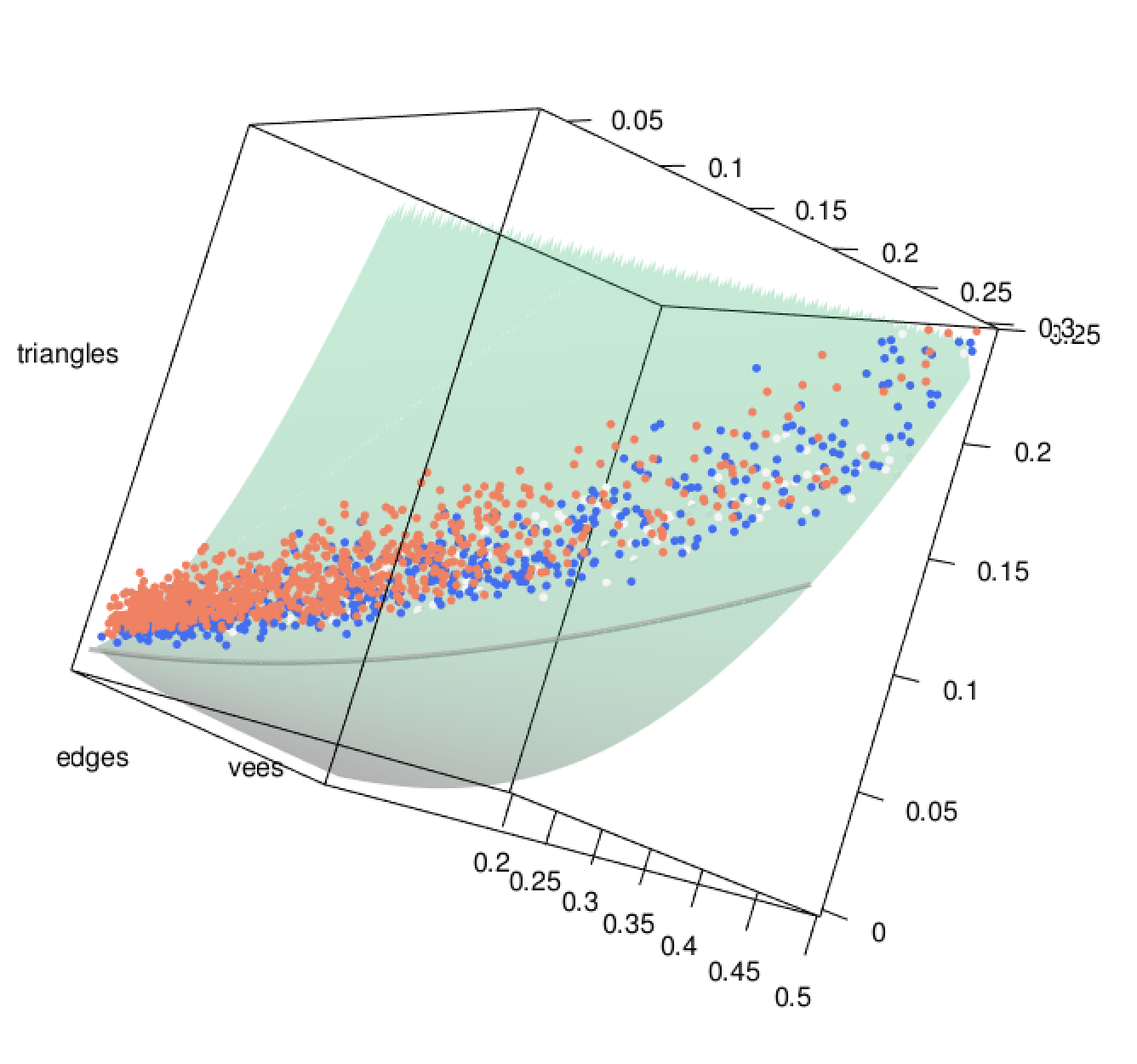
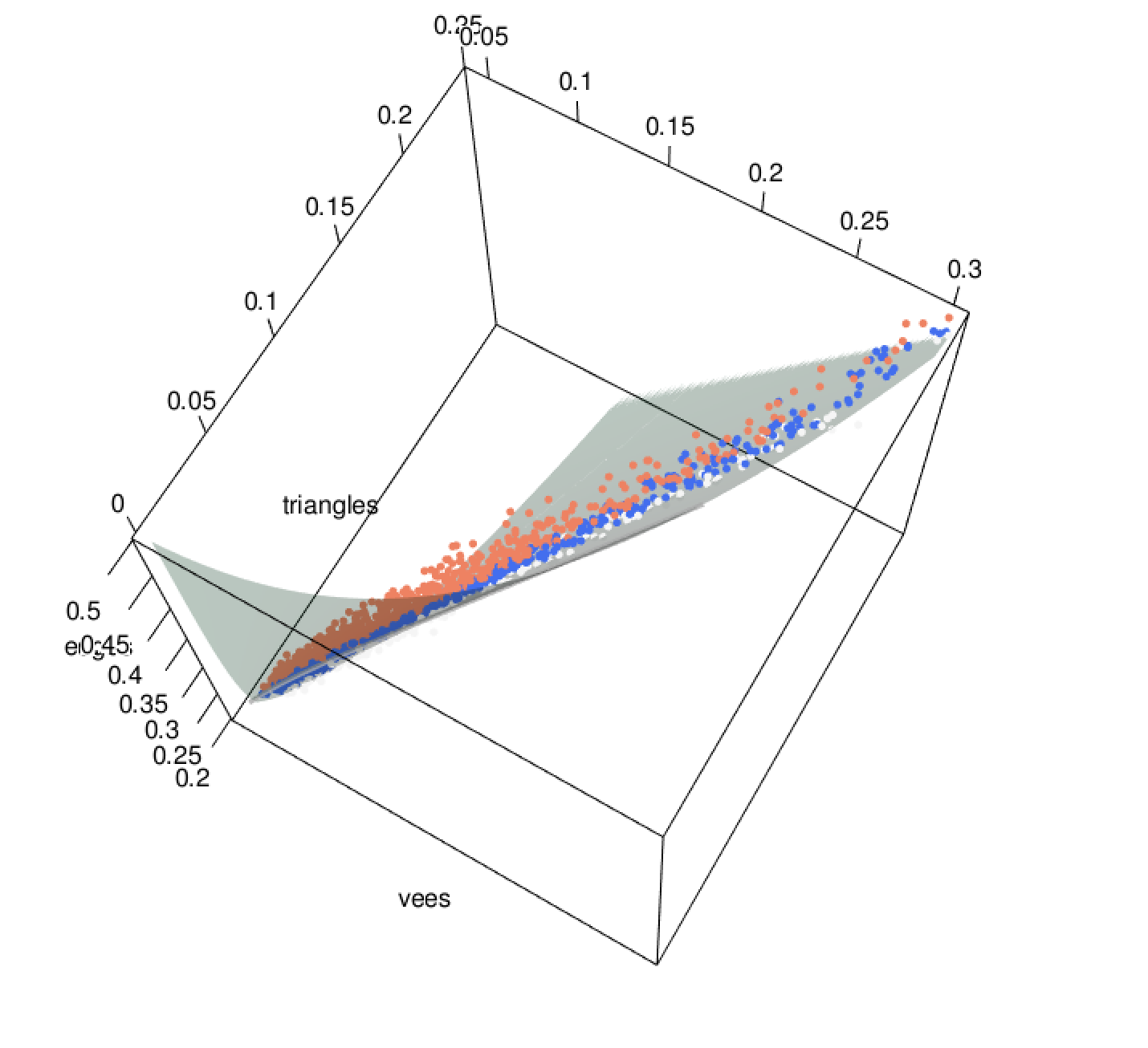
Refer to caption Refer to caption
Fig 1: Top row: Two different views of 3-dimensional plots of the triangle, vee, and edge densities of a collection of Facebook subnetworks. Each point represents a single subnetwork, the induced graph of the friends of a single Facebook user (ego), in the fb100 data. Each subnetwork in this collection has between 20 and 40 nodes. The coordinates (E^,V^,T^)(\widehat{E},\widehat{V},\widehat{T}) of a given point are the relative frequencies of edges, vees, and triangles in the network. The points are colored according to the p-value of the EZ score test: red, smaller than 10−510^{-5}; blue, in the range (10−5,10−2)(10^{-5},10^{-2}); white, larger than 10−210^{-2}. The shaded surface indicates the subfamily of degree-corrected stochastic block models for which χe​v=T−(V/E)3=0\chi_{ev}=T-(V/E)^{3}=0, and no community structure is present. The curve on the surface, visible in the left plot, corresponds to the subfamily of Erdős-Rényi graphs where (E,V,T)=(p,p2,p3)(E,V,T)=(p,p^{2},p^{3}). Qualitatively, we see that even the points that lie relatively close to the Erdős-Zuckerberg surface χe​z=0\chi_{ez}=0, are far from the Erdős-Rényi curve, which may be attributed to degree heterogeneity. Bottom row: Typical Facebook subnetworks with small and large p-values. The left graph, with an EZ score of 8.25 and p-value of 10−1610^{-16}, has clear community structure. The right graph, with an EZ score of 0.498 and p-value of 0.62, exhibits no community structure.

In the present paper we take a statistical approach to distinguishing graphs with community structure from unstructured random graphs using only small subgraph frequencies, framing the problem in terms of statistical testing. The starting point for our analysis is the degree-corrected stochastic block model, a simple generative model for random networks that captures two salient properties that are observed empirically in social networks and other data—community structure and degree heterogeneity. While the precise specification of the model is deferred to the following section, it is characterized by a few key parameters, including the number of communities k≥1k\geq 1, the within-community connectivity probability aa, and the between-community connectivity probability bb. For random networks, we define

χe​z=T−(VE)3,\chi_{ez}=T-\left(\frac{V}{E}\right)^{3},

where now EE, VV, and TT are the expected densities of edges ( ), vees ( ), and triangles ( ) in the graph. A simple calculation, which we present in the following section, shows that under the degree-corrected stochastic block model,

χe​z=(k−1)​(a−bk)3.\chi_{ez}=(k-1)\left(\frac{a-b}{k}\right)^{3}. (1.1)

We thus see that χe​z=0\chi_{ez}=0 if and only if the network has no communities, under the assumed model, meaning that a=ba=b or k=1k=1. In particular, an Erdős-Rényi random graph with edge probability pp satisfies

χe​z=p3−(p2p)3=0.\chi_{ez}=p^{3}-\left(\frac{p^{2}}{p}\right)^{3}=0.

Since χe​z=0\chi_{ez}=0 distinguishes unstructured random networks from those with community structure, within the large class of degree-corrected stochastic block models, we refer to χe​z\chi_{ez} as the Erdős-Zuckerberg characteristic, or the EZ characteristic, for short.

Starting from the simple relation in (1.1), this paper explores the mathematical, statistical, and empirical properties of the Erdős-Zuckerberg characteristic as a test for global community structure. We find that this simple functional has remarkable properties, both theoretically and empirically. We develop a testing framework for the null hypothesis corresponding to χe​z=0\chi_{ez}=0, and analyze its power and scaling behavior. Empirically, we find that the test is effective on the types of Facebook subnetworks studied by Ugander et al., (2013). In particular, graphs with small p-values under this test exhibit clear community structure, while unstructured subnetworks typically lie close to the cubic surface defined by the invariant χe​z=0\chi_{ez}=0, with correspondingly large p-values; see Figure 1. However, even the unstructured subnetworks are relatively far from the curve in this surface traced out by the Erdős-Rényi subfamily, and a closely related test based on an Erdős-Rényi null hypothesis is ineffective.

In related work, Mossel et al., (2012) prove a Poisson limit law for counts of cycles in stochastic block models, and Maugis et al., (2017) consider the use of small subgraph counts to test whether a collection of networks is drawn from a known graphon null model. Bubeck et al., (2014) study tests based on signed triangles for distinguishing Erdős-Rényi graphs from random geometric graphs in the dense regime. Banerjee, (2016) and Banerjee and Ma, (2017) study tests based on signed circles and establish a relation to the likelihood ratio statistic for stochastic block models. Ambroise and Matias, (2012) and Allman et al., (2011) study moment estimators for the parameters of stochastic block models; these estimators were used recently by Kloumann et al., (2017) in the context of seed set expansion and node ranking in personalized search.

In the following section we provide further detail on the relation (1.1), which is the key equation in our testing approach, and then develop a central limit theorem for this characteristic based on empirical estimates of the densities of edges, vees and triangles. The power and scaling behavior of the resulting test is analyzed in Section 2.2. In Section 2.4 we comment on a related test when the null model is chosen to be an Erdős-Rényi model rather than a configuration model, the essential difference being degree heterogeneity. The discussion in this section sheds light on the empirical findings shown in Figure 1, where the Facebook subnetworks are relatively far from the Erdős-Rényi subfamily, but close to the surface defined by χe​z=0\chi_{ez}=0. Section 3 gives illustrations of our testing framework on Facebook social networks, citations from statistics journal articles, and stock returns of companies on the S&P 500. In each of these settings, we find that the Erdős-Zuckerberg test gives interesting and interpretable results, and is effective at identifying community structure using only the local information available in two and three node subgraph statistics. Finally, in the supplementary material, we give some extensions of the Erdős-Zuckerberg characteristic and present the proofs of the results of the paper. Section A introduces a rigorous framework of tests for neighborhood graphs. Section B considers correlation structures for multivariate Gaussian data, and derives an analogous test for community structure under this model.

2 The Erdős-Zuckerberg Test

One of the most popular network models of community structure is the degree-corrected stochastic block model (DCBM) (Dasgupta et al.,, 2004; Karrer and Newman,, 2011). Under this model, a random adjacency matrix AA is generated according to Ai​j|θi​j∼Bernoulli​(θi​j)A_{ij}\,|\,\theta_{ij}\sim\text{Bernoulli}(\theta_{ij}) independently for each edge (i,j)(i,j), where the mean parameters θi​j\theta_{ij} have a blockwise low rank structure that models degree heterogeneity and community structure. For community structure, latent variables Zi∼Uniform​([k])Z_{i}\sim\text{Uniform}([k]) are generated independently for each node ii, where the integer k≥1k\geq 1 is the number of communities. For degree heterogeneity, variables Wi∼𝒲W_{i}\sim\mathcal{W} are generated independently for each node from a distribution 𝒲\mathcal{W}; the value WiW_{i} can be thought of as a measure of the “sociability” of node ii. Conditional on ZZ and WW, the mean parameters θi​j\theta_{ij} are then given by

θi​j|W,Z={Wi​Wj​a,Zi=Zj,Wi​Wj​b,Zi≠Zj,\theta_{ij}\,|\,W,Z=\begin{cases}W_{i}W_{j}a,&Z_{i}=Z_{j},\\ W_{i}W_{j}b,&Z_{i}\neq Z_{j},\end{cases} (2.1)

where aa is the within-community connectivity probability, and bb is the between-community connectivity probability.

Thus, the distribution of {Ai​j}1≤i<j≤n\{A_{ij}\}_{1\leq i<j\leq n} is fully determined by the parameters aa, bb, kk and the distribution 𝒲\mathcal{W}. The parameterization (2.1) is not identifiable, since the model is invariant to multiplying aa and bb by some arbitrary number t>0t>0, and dividing each WiW_{i} by t\sqrt{t}. Thus, without loss of generality, we introduce the constraint

𝔼⁡(W2)=1,{\mathbb{E}}(W^{2})=1, (2.2)

for the distribution 𝒲\mathcal{W}, so that the parameters aa and bb are uniquely determined.

The problem of community detection in the setting of the DCBM has been well studied in the literature (Lei and Rinaldo,, 2015; Gulikers et al.,, 2015; Zhao et al.,, 2012; Jin,, 2015; Chen et al.,, 2015). Gao et al., (2016) derive the minimax rate of the problem with respect to the Hamming loss. All of this work assumes there exists a clustering structure in the model and the number of clusters kk is given. In the current paper, we shift the focus to testing for community structure, without estimating kk or the clusters themselves. Under the DCBM, the lack of such structure is equivalent to k=1k=1 or a=ba=b.

The following result is central to our testing procedure and analysis.

Proposition 2.1.

Define the population edge, vee, and triangle probabilitities by

E\displaystyle E =\displaystyle= ℙ⁡(A12=1),\displaystyle{\mathbb{P}}(A_{12}=1), (2.3)
V\displaystyle V =\displaystyle= ℙ⁡(A12​A13=1),\displaystyle{\mathbb{P}}(A_{12}A_{13}=1), (2.4)
T\displaystyle T =\displaystyle= ℙ⁡(A12​A13​A23=1).\displaystyle{\mathbb{P}}(A_{12}A_{13}A_{23}=1). (2.5)

Then under the degree-corrected stochastic block model (2.1) and assuming the identifiability condition (2.2), we have

E\displaystyle E =\displaystyle= (𝔼​W)2​(1k​a+k−1k​b),\displaystyle({\mathbb{E}}W)^{2}\left(\frac{1}{k}a+\frac{k-1}{k}b\right), (2.6)
V\displaystyle V =\displaystyle= (𝔼​W)2​(1k​a+k−1k​b)2,\displaystyle({\mathbb{E}}W)^{2}\left(\frac{1}{k}a+\frac{k-1}{k}b\right)^{2}, (2.7)
T\displaystyle T =\displaystyle= 1k2​a3+3​(k−1)k2​a​b2+(k−1)​(k−2)k2​b3.\displaystyle\frac{1}{k^{2}}a^{3}+\frac{3(k-1)}{k^{2}}ab^{2}+\frac{(k-1)(k-2)}{k^{2}}b^{3}. (2.8)

From these relations, it follows that

χe​z≡T−(VE)3=(k−1)​(a−b)3k3.\chi_{ez}\equiv T-\left(\frac{V}{E}\right)^{3}=\frac{(k-1)(a-b)^{3}}{k^{3}}. (2.9)
Proof.

The identities follow from direct calculation. For example, because {Wi}\{W_{i}\} and {Zi}\{Z_{i}\} are sampled independently, we have that

E=𝔼⁡(A12)\displaystyle E={\mathbb{E}}(A_{12}) =𝔼⁡(𝔼⁡(A12|Z1,Z2,W1,W2))\displaystyle={\mathbb{E}}\bigl({\mathbb{E}}(A_{12}\,|\,Z_{1},Z_{2},W_{1},W_{2})\bigr)
=𝔼⁡(W1​W2​(a​𝟙​(Z1=Z2)+b​𝟙​(Z1≠Z2))CLOSE\displaystyle={\mathbb{E}}\left(W_{1}W_{2}\bigl(a\mathbbm{1}(Z_{1}=Z_{2})+b\mathbbm{1}(Z_{1}\neq Z_{2}\bigr)\right)
=𝔼⁡(W1​W2​(a​1k+b​k−1k))\displaystyle={\mathbb{E}}\left(W_{1}W_{2}\Bigl(a\frac{1}{k}+b\frac{k-1}{k}\Bigr)\right)
=(𝔼​W)2​(a​1k+b​k−1k).\displaystyle=({\mathbb{E}}W)^{2}\Bigl(a\frac{1}{k}+b\frac{k-1}{k}\Bigr).

Equations (2.7) and (2.8) are derived similarly, using the constraint 𝔼⁡(W2)=1{\mathbb{E}}(W^{2})=1. The relation (2.9) is then seen to hold after some algebra. ∎

The relation (2.9) implies that k=1k=1 or a=ba=b if and only if χe​z=0\chi_{ez}=0, which characterizes whether or not the network has community structure. When χe​z=0\chi_{ez}=0, the model is reduced to θi​j=a​Wi​Wj\theta_{ij}=a\/W_{i}W_{j}, which is also recognized as the configuration model (van der Hofstad,, 2016), and closely related to the Chung-Lu model of random graphs with expected degrees (Chung and Lu,, 2002). If χe​z>0\chi_{ez}>0, then the network has an assortative clustering structure; such a network will induce more triangles compared with the configuration model. Conversely, the network will have disassortative clustering structure if χe​z<0\chi_{ez}<0, in which case there will be fewer triangles. We see both types of structure in our empirical studies, described below.

2.1 The EZ test

We now develop a statistical test for the null hypothesis H0:χe​z=0H_{0}:\chi_{ez}=0. The empirical versions of relations (2.3)–(2.5) are

E^\displaystyle\widehat{E} =\displaystyle= 1(n2)​∑1≤i<j≤nAi​j,\displaystyle\frac{1}{{n\choose 2}}\sum_{1\leq i<j\leq n}A_{ij},
V^\displaystyle\widehat{V} =\displaystyle= 1(n3)​∑1≤i<j<l≤nAi​j​Ai​l+Ai​j​Aj​l+Ai​l​Aj​l3,\displaystyle\frac{1}{{n\choose 3}}\sum_{1\leq i<j<l\leq n}\frac{A_{ij}A_{il}+A_{ij}A_{jl}+A_{il}A_{jl}}{3},
T^\displaystyle\widehat{T} =\displaystyle= 1(n3)​∑1≤i<j<l≤nAi​j​Ai​l​Aj​l.\displaystyle\frac{1}{{n\choose 3}}\sum_{1\leq i<j<l\leq n}A_{ij}A_{il}A_{jl}.

Therefore, we can reject the null hypothesis once the magnitude of the plug-in test statistic

χ^e​z≡T^−(V^/E^)3\widehat{\chi}_{ez}\equiv\widehat{T}-\left({\widehat{V}}/{\widehat{E}}\right)^{3} (2.10)

passes a threshold. The following result gives the asymptotic distribution of χ^e​z\widehat{\chi}_{ez}, and allows us to set the threshold and significance level of the test.

Theorem 2.2.

Assume 𝔼​W4=O⁡(1){\mathbb{E}}W^{4}=O(1) and n−1≪a≍b≪n−2/3n^{-1}\ll a\asymp b\ll n^{-2/3}. Suppose

δ=limn(k−1)​(a−b)36​(nk⁡(a+(k−1)​b))3/2∈[0,∞).\delta=\lim_{n}\frac{(k-1)(a-b)^{3}}{\sqrt{6}}\left(\frac{n}{k(a+(k-1)b)}\right)^{3/2}\in[0,\infty). (2.11)

Then the following three convergence results hold:

(n3)​χ^e​zT^\displaystyle\frac{\sqrt{{n\choose 3}}\;\widehat{\chi}_{ez}}{\sqrt{\widehat{T}}} ↝N⁡(δ,1)\displaystyle\leadsto N(\delta,1) (2.12)
(n3)​χ^e​z(V^/E^)3\displaystyle\frac{\sqrt{{n\choose 3}}\;\widehat{\chi}_{ez}}{\sqrt{\left({\widehat{V}}/{\widehat{E}}\right)^{3}}} ↝N⁡(δ,1)\displaystyle\leadsto N(\delta,1) (2.13)
2​(n3)​(T^−(V^/E^)3/2)\displaystyle{\textstyle 2{\sqrt{{n\choose 3}}}\left(\sqrt{\widehat{T}}-\left({\widehat{V}}/{\widehat{E}}\right)^{3/2}\right)} ↝N⁡(δ,1).\displaystyle\leadsto N(\delta,1). (2.14)

Theorem 2.2 shows that the asymptotic distribution of the testing statistic is Gaussian. We can either normalize (n3)​χ^e​z\sqrt{{n\choose 3}}\,\widehat{\chi}_{ez} by T^\sqrt{\widehat{T}} or by (V^/E^)3\sqrt{\left({\widehat{V}}/{\widehat{E}}\right)^{3}}. However, it may be possible that T^=0\widehat{T}=0 or V^=0\widehat{V}=0. Thus, we prefer the normalization by 12​(T^+(V^/E^)3/2)\frac{1}{2}\Bigl(\sqrt{\widehat{T}}+\left({\widehat{V}}/{\widehat{E}}\right)^{3/2}\Bigr), which results in (2.14). This square-root normalization can be seen as a form of variance-stabilizing transformation (Anscombe,, 1948).

The assumption n−1≪a≍b≪n−2/3n^{-1}\ll a\asymp b\ll n^{-2/3} controls the sparsity of the graph. It covers the most interesting nontrivial range studied in the community detection literature, which is from n−1n^{-1} to n−1​log⁡nn^{-1}\log n. Below the order of n−1n^{-1}, the graph is so sparse that consistent community detection is not possible (Mossel et al.,, 2012; Mossel et al.,, 2013). Above the order of n−1​log⁡nn^{-1}\log n, the graph carries sufficient information and strong consistency of community detection can be proved (Bickel and Chen,, 2009; Abbe et al.,, 2016).

2.2 Power of the EZ test

The mean of the asymptotic distribution is given in (2.11). When χe​z=0\chi_{ez}=0, we get δ=0\delta=0, and the asymptotic distribution is N⁡(0,1)N(0,1). Therefore, the p-value of the test can be calculated from the standard Gaussian quantile function. When k→∞k\rightarrow\infty, the order of (2.11) is

δ≍(n​(a−b)2k4/3​(a+b))3/2.\delta\asymp\left(\frac{n(a-b)^{2}}{k^{4/3}(a+b)}\right)^{3/2}.

This leads to the following result on the power of the test.

Theorem 2.3.

Assume 𝔼​W4=O⁡(1){\mathbb{E}}W^{4}=O(1) and n−1≪a≍b≪n−2/3n^{-1}\ll a\asymp b\ll n^{-2/3}. Suppose

n​(a−b)2k4/3​(a+b)⟶∞.\frac{n(a-b)^{2}}{k^{4/3}(a+b)}\longrightarrow\infty. (2.15)

Then, for any constant t≍1t\asymp 1, we have

ℙ⁡(|2​(n3)​(T^−(V^/E^)3/2)|>t)→1.{\mathbb{P}}\left(\bigl|{\textstyle 2{\sqrt{{n\choose 3}}}\left(\sqrt{\widehat{T}}-\left({\widehat{V}}/{\widehat{E}}\right)^{3/2}\right)}\bigr|>t\right)\rightarrow 1.

This result characterizes the power of the proposed test under the condition (2.15). Conditions of a similar form are common in the community detection literature. For example, in the setting of the DCBM, Gao et al., (2016) require n​(a−b)2k5​(a+b)→∞\frac{n(a-b)^{2}}{k^{5}(a+b)}\rightarrow\infty for minimax optimal community detection. The scaling in (2.15) is the same except for a much weaker dependence on kk, indicating that the problem of testing for network structure may be statistically easier than network clustering.

When k=O⁡(1)k=O(1), the condition (2.15) reduces to n​(a−b)2a+b→∞\frac{n(a-b)^{2}}{a+b}\rightarrow\infty. The optimality of this condition has been studied in the setting of the stochastic block model, which is a special setting of the DCBM. For example, when k=2k=2, Mossel et al., (2012) show that distinguishing between an Erdős-Rényi model and a stochastic block model is impossible when n​(a−b)22​(a+b)<1\frac{n(a-b)^{2}}{2(a+b)}<1. On the other hand, Mossel et al., (2012); Banerjee, (2016); Banerjee and Ma, (2017) show that when n​(a−b)22​(a+b)>1\frac{n(a-b)^{2}}{2(a+b)}>1, there exists a consistent test to distinguish Erdős-Rényi model and a stochastic block model. For a growing number of communities kk, the impossibility result was extended by Banks et al., (2016), showing that an Erdős-Rényi model is indistinguishable from a stochastic block model if n​(a−b)2k​log⁡k​(a+b)\frac{n(a-b)^{2}}{k\log k(a+b)} is bounded by some constant. Here, we simplify the expression by assuming that a≍ba\asymp b.

In this paper, we study the more general setting of the DCBM. Therefore, established lower bounds for the stochastic block model also apply here. The Erdős-Zuckerberg test requires the condition n​(a−b)2k4/3​(a+b)→∞\frac{n(a-b)^{2}}{k^{4/3}(a+b)}\rightarrow\infty, which is nearly optimal compared to these lower bound results.

2.3 Computation of the test statistic for sparse networks

Sparse matrix multiplication can be used to efficiently compute the test statistic χ^e​z\widehat{\chi}_{ez}. If AA is the binary adjacency matrix of the graph, then (Al)i​j(A^{l})_{ij} is the number of paths of length ll from ii to jj. It follows that

E^\displaystyle\widehat{E} =12​(n2)​⟨𝟙,A⟩\displaystyle=\frac{1}{2{n\choose 2}}\left\langle\mathbbm{1},\,A\right\rangle (2.16)
V^\displaystyle\widehat{V} =16​(n3)​(⟨𝟙,A2⟩−tr(A2))\displaystyle=\frac{1}{6{n\choose 3}}\left(\left\langle\mathbbm{1},\,A^{2}\right\rangle-\mathop{\rm tr}(A^{2})\right) (2.17)
T^\displaystyle\widehat{T} =16​(n3)​tr(A3)\displaystyle=\frac{1}{6{n\choose 3}}\mathop{\rm tr}(A^{3}) (2.18)

where tr(⋅)\mathop{\rm tr}(\cdot) denotes the matrix trace, ⟨A,B⟩=tr(AT​B)\left\langle A,\,B\right\rangle=\mathop{\rm tr}(A^{T}B) is the matrix inner product, and the symbol 𝟙\mathbbm{1} denotes a matrix of all ones. These relations were used to efficiently calculate the test statistic in the experiments presented in Section 3.

2.4 An EZ test for stochastic block models

When 𝒲\mathcal{W} becomes a delta measure on 11, the DCBM reduces to the SBM. A simplified Erdős-Zuckerberg characteristic holds in this setting, which only requires the estimation of the edge and the triangle densities.

Proposition 2.4.

When 𝔼​W=𝔼​W2=1{\mathbb{E}}W={\mathbb{E}}W^{2}=1, we have

T−E3=(k−1)​(a−b)3k3.T-E^{3}=\frac{(k-1)(a-b)^{3}}{k^{3}}.

This result is easily derived from Proposition 2.9 via the relation V=E2V=E^{2} when 𝔼​W=1{\mathbb{E}}W=1 by (2.6) and (2.7). Analogous results to Theorem 2.2 and Theorem 2.3 also hold for the plug-in statistic T^−E^3\widehat{T}-\widehat{E}^{3} under the SBM. In particular, 2​(n3)​(T^−E^3)↝N⁡(δ,1)2\sqrt{{n\choose 3}}\left(\sqrt{\widehat{T}}-\sqrt{\widehat{E}^{3}}\right)\leadsto N(\delta,1), where δ\delta shares the same definition in (2.11). Moreover, the power of the corresponding test goes to one under the alternative hypothesis of a stochastic block model with the same signal-to-noise ratio condition (2.15). See Gao and Lafferty, (2017) for further detail.

While the form of this test is similar, there is a significant difference between the Erdős-Zuckerberg characterizations for the SBM and the DCBM. Consider a DCBM with k=1k=1—in other words, a configuration model. By Proposition 2.9, T−(V/E)3=0T-\left({V}/{E}\right)^{3}=0. However, a simple calculation using the expressions in (2.6)–(2.8) gives

T−E3=a3​(1−(1−Var​(W))3).T-E^{3}=a^{3}(1-(1-\text{Var}(W))^{3}).

Thus, as long as Var​(W)>0\text{Var}(W)>0, the statistic satisfies T−E3>0T-E^{3}>0.

This calculation shows that while the configuration model is the benchmark of triangle frequency used in our EZ test, this model will have more triangles compared with the benchmark of an Erdős-Rényi model. This phenomenon is apparent in the plots of Figure 1, where the surface indicates the subfamily of degree-corrected stochastic block models for which χe​v=T−(V/E)3=0\chi_{ev}=T-(V/E)^{3}=0, and no community structure is present. The curve on the surface, visible in the upper left plot, corresponds to the subfamily of Erdős-Rényi graphs where (E,V,T)=(p,p2,p3)(E,V,T)=(p,p^{2},p^{3}). Each point represents a Facebook subnetwork; the points that lie relatively close to the Erdős-Zuckerberg surface χe​z=0\chi_{ez}=0 are still far from the Erdős-Rényi curve. This is attributable to degree heterogeneity in the Facebook networks, which is captured by the configuration model.

3 Examples

In this section we describe experiments with the proposed testing framework on three types of data: social networks, citations from journal articles, and stock returns of companies on the S&P 500. In each setting, we demonstrate the performance of the test qualitatively, by showing examples of the networks that have large and small p-values. For each of the three data sets, we find that the Erdős-Zuckerberg test gives interesting and intepretable results, and is effective at identifying community structure.

3.1 Facebook friend networks

The current work was motivated by the empirical findings of Ugander et al., (2013), which compared the distributions of 3-node and 4-node subgraphs of Facebook friend networks to those obtained under an Erdős-Rényi baseline model. In this section we apply our testing method to Facebook subnetworks similar to those used in this previous work.


Fig 2: Facebook neighborhood graphs, each with between 30 and 40 nodes, extracted from the Carnegie Mellon University portion of the Facebook 100 dataset. Top: 12 randomly selected graphs with p-values smaller than 10−1210^{-12}, under the EZ test. Bottom: 12 graphs with p-values larger than 0.1. The results for other universities are similar. Community structure is readily apparent in the top graphs, and lacking in the bottom graphs.

The data we use are from the “Facebook 100” dataset, comprised of Facebook friend networks from 100 U.S. universities, collected in 2005. In addition to the friend relations user attributes such as dorm, gender, graduation year, and academic major are included in the data; however, we do not use these attributes in our analysis.

The data are divided into separate networks for each of the 100 universities. For a given university, we form the induced graph of a given user ee by forming an adjacency matrix A(e)=(Ai​j(e))A^{(e)}=\bigl(A^{(e)}_{ij}\bigr) with respect to the friends of ee, with Ai​j(e)=1A^{(e)}_{ij}=1 if ii is a friend of jj (or vice-versa), and Ai​j(e)=0A^{(e)}_{ij}=0 otherwise. A discussion of the inferential properties of selecting neighborhood graphs this way is given in the supplementary material (see Section A).

We display sample results for the Carnegie Mellon University subnetwork; the results for other universities are qualitatively very similar. Restricting to subgraphs having between 30 and 40 nodes results in 556 graphs for the CMU subnetwork. The p-values were computed according to the Erdős-Zuckerberg test implied by equation (2.14). A histogram of these 556 p-values is displayed in Figure 3, where it is seen that most of the p-values are very small, indicating significant structure. Figure 2 shows 12 randomly selected graphs having large (>0.1>0.1) and small (<10−12<10^{-12}) p-values under the test. Community structure is readily apparent in the graphs with small p-values. Structure is absent in the graphs with large p-values, while they clearly have degree heterogeneity, as modeled by the configuration model.

   
Fig 3: Histograms of p-values of the Facebook graphs and journal citation graphs. Left: histogram of the 556 neighborhood graphs in the Carnegie Mellon subnetwork that have between 30 and 40 nodes. Most of the graphs have significant community structure according to the EZ test. Right: histogram of the p-values for subnetworks of the citation data. In the case, the p-values are typically large, indicating a lack of community structure.

3.2 Citation networks from statistics journals

The data used to illustrate the proposed test in this section are associated with citations from several statistics journals, including the Annals of Statistics, Biometrika, the Journal of the American Statistical Association, and the Journal of the Royal Statistical Society, Series B. The citations are from papers published between 2003 and 2012 (Ji and Jin,, 2016).

We work with the “giant component” of the citation network from this dataset, where each node in the network corresponds to one of 2,654 authors. A directed edge from author ii to jj indicates that author ii has cited one or more papers by author jj. We extract subnetworks A(a)=(Ai​j(a))A^{(a)}=(A^{(a)}_{ij}) for a given author aa. This graph is over the authors cited by aa, with Ai​j(a)=1A^{(a)}_{ij}=1 if ii cites jj (or vice-versa), and Ai​j(a)=0A^{(a)}_{ij}=0 otherwise.

Fig 4: Two networks from the statistics citation data. Top: induced network for the statistician Michael I. Jordan (Berkeley), with a small p-value of 9×10−59\times 10^{-5} and an EZ score of 3.913.91. Clustering structure is evident in the subnetwork, with three groups that might be labeled “nonparametric Bayes,” “statistical learning theory” and “North Carolina statistics.” Bottom: network for Christopher Genovese (Carnegie Mellon), with a p-value of 2×10−122\times 10^{-12}. The EZ score for this network has a negative value of −7.03-7.03, indicating a model with a<ba<b, and a smaller number of triangles compared with a configuration model. The nodes on the periphery are highly connected to the inner cluster, but not highly connected among themselves. (Some of the node labels have been removed for better readability.)

For these data, 387 authors have induced graphs of size 15 or larger. A histogram of the p-values for these graphs is shown in the right plot of Figure 3. This shows that the p-values are much closer to uniform, indicating a general lack of community structure, compared with the Facebook networks. Two sample graphs that have small p-values are shown in Figure 4. The top graph shows the induced graph for Berkeley statistician Michael I. Jordan (Berkeley). This graph has a p-value of 9×10−59\times 10^{-5} and an EZ score of 3.913.91. Three communities are apparent in the subnetwork; knowledge of the authors in these groups leads one to interpret them as “nonparametric Bayes,” “statistical learning theory” and “North Carolina statistics.” A similar discovery is also made by Jin et al., (2017) with a different analysis under a mixed-membership model. The bottom network is interesting because it has a large negative EZ score of −7.03-7.03. This is the network associated with Christopher Genovese, from Carnegie Mellon University. The dense core of the network includes researchers from CMU, and other statisticians who work in similar areas. The nodes on the periphery are highly connected to the inner cluster, but very weakly connected among themselves. Thus, researchers in this outer group tend not to cite each other, but cite (or are cited by) researchers in the inner group.

3.3 Correlations among stocks on the S&P 500

In this third illustration, we treat correlations among the returns of stocks on the S&P 500. The data are derived from prices posted on the Yahoo Finance site, finance.yahoo.com. The daily closing prices were obtained for 452 stocks that consistently were in the S&P 500 index between January 1, 2003 through January 1, 2011. We restrict to the subset of the data between January 1, 2003 to January 1, 2008, before the onset of the 2008–2009 financial crisis. After this event, stocks tended to become much more tightly correlated as investors became more cautious. We consider the variables Xt,j=log⁡(St,j/St​−​1,j)X_{t,j}=\log(S_{t,j}/S_{t−1,j}) where St,jS_{t,j} denotes the closing price of stock jj on day tt. The 452 stocks are categorized into 10 Global Industry Classification Standard (GICS) sectors, including Consumer Discretionary (70 stocks), Consumer Staples (35 stocks), Energy (37 stocks), Financials (74 stocks), Health Care (46 stocks), Industrials (59 stocks), Information Technology (64 stocks), Materials (29 stocks), Telecommunications Services (6 stocks), and Utilities (32 stocks).

Stocks within a sector are generally strongly correlated–stocks within an industry tend to move together. For a given company, we form a subnetwork that is analogous to the Facebook subnetworks considered in Section 3.1 (see also Section A). Specifically, we create an edge Ai​j=1A_{ij}=1 between companies ii and jj if their returns are strongly correlated, and each is strongly correlated with the given company. We take “strongly correlated” to mean a Spearman rank correlation in the 95th percentile, which is a correlation above 0.45.

Example networks are shown in Figure 5; three have apparent community structure, one shows no apparent community structure. For example, the upper right figure shows the correlation graph for Consol Energy, which is based outside of Pittsburgh, PA, and has interests in coal and natural gas production; its customers include electric utilities and steel mills.11 1 Wikipedia, https://en.wikipedia.org/wiki/Consol_Energy Two communities are seen in the graph, with companies from the Energy sector (including oil companies and other energy companies) and the Materials sector (including the US Steel Corporation and Alcoa Inc.).

SCANA Corp, p=1.7×10⁻⁷p=1.7\times 10^{-7} CONSOL Energy, p=0.0043p=0.0043
Agilent Technologies, p=0.0095p=0.0095 Family Dollar Stores, p=0.97p=0.97
Fig 5: Example correlation graphs for companies on the S&P 500. For a given company we form a subnetwork among all companies having high correlation (larger than 0.450.45) with that company. We then compute the EZ score and p-value for this correlation graph. This figure shows four representative subnetworks, three with relatively small p-values and cluster structure, and one with a large p-value and no apparent cluster structure. The node labels are the GICS industry of the company corresponding to that node.

4 Summary

Our results show how global structural characteristics of networks can be inferred from local subgraph frequencies, without requiring the global community structure to be explicitly estimated. We develop a testing framework based on the simple invariant χe​z=T−(V/E)3=0\chi_{ez}=T-(V/E)^{3}=0 satisfied by all configuration models that lack community structure. Our theory indicates that the signal-to-noise ratio required for the hypothesis test to find community structure, when it is present, is weaker than what is required by existing procedures that rely on explicitly estimating the communities. Experiments with social network data, scientific citations and equity returns show that the test can be very effective. Our findings shed light on the question of how global graph properties are reflected in local subgraph statistics. Lower bounds for detecting community structure, as well as the development of more powerful tests for particular settings such as Gaussian data and time series, are promising directions for further study.

Acknowledgements

The authors thank Rina Barber and Tracy Ke for many helpful comments on this work, including the suggestion of the configuration null model. We also thank Fengnan Gao for suggesting the martingale central limit theorem in Hall and Heyde, (2014), and Scarlett Li for help with the simulations. The research of JL is supported in part by NSF grant DMS-1513594 and ONR grant N00014-12-1-0762. The research of CG is supported in part by NSF grant DMS-1712957.

References

  • Abbe et al., (2016) Abbe, E., Bandeira, A. S., and Hall, G. (2016). Exact recovery in the stochastic block model. Information Theory, IEEE Transactions on, 62(1):471–487.
  • Allman et al., (2011) Allman, E. S., Matias, C., and Rhodes, J. A. (2011). Parameter identifiability in a class of random graph mixture models. Journal of Statistical Planning and Inference, 141(5):1719–1736.
  • Ambroise and Matias, (2012) Ambroise, C. and Matias, C. (2012). New consistent and asymptotically normal parameter estimates for random graph mixture models. Journal of the Royal Statistical Society Series B, 74(1):3–35.
  • Anscombe, (1948) Anscombe, F. J. (1948). The transformation of Poisson, binomial and negative-binomial data. Biometrika, 35(3/4):246–254.
  • Arias-Castro et al., (2011) Arias-Castro, E., Candès, E., and Durand, A. (2011). Detection of an anomalous cluster in a network. Ann. Statist., 39(1):278–304.
  • Arias-Castro and Verzelen, (2014) Arias-Castro, E. and Verzelen, N. (2014). Community detection in dense random networks. Ann. Statist., 42(3):940–969.
  • Banerjee, (2016) Banerjee, D. (2016). Contiguity and non-reconstruction results for planted partition models: the dense case. arXiv preprint arXiv:1609.02854.
  • Banerjee and Ma, (2017) Banerjee, D. and Ma, Z. (2017). Optimal hypothesis testing for stochastic block models with growing degrees. working manuscript.
  • Banks et al., (2016) Banks, J., Moore, C., Neeman, J., and Netrapalli, P. (2016). Information-theoretic thresholds for community detection in sparse networks. In Conference on Learning Theory, pages 383–416.
  • Barabási and Albert, (1999) Barabási, A. L. and Albert, R. (1999). Emergence of scaling in random networks. Science, 286(5439):509–512.
  • Bickel and Chen, (2009) Bickel, P. J. and Chen, A. (2009). A nonparametric view of network models and Newman–Girvan and other modularities. Proceedings of the National Academy of Sciences, 106(50):21068–21073.
  • Bollobás, (2001) Bollobás, B. (2001). Random Graphs. Cambridge University Press.
  • Bubeck et al., (2014) Bubeck, S., Ding, J., Eldan, R., and Rácz, M. (2014). Testing for high-dimensional geometry in random graphs. arXiv:1411.5713.
  • Bunea et al., (2015) Bunea, F., Giraud, C., and Luo, X. (2015). Minimax optimal variable clustering in g-models via cord. arXiv preprint arXiv:1508.01939.
  • Chen et al., (2015) Chen, Y., Li, X., and Xu, J. (2015). Convexified modularity maximization for degree-corrected stochastic block models. arXiv preprint arXiv:1512.08425.
  • Chung and Lu, (2002) Chung, F. and Lu, L. (2002). The average distance in random graphs with given expected degrees. Proceedings of National Academy of Sciences (PNAS), 99(25):15879–15882.
  • Dasgupta et al., (2004) Dasgupta, A., Hopcroft, J. E., and McSherry, F. (2004). Spectral analysis of random graphs with skewed degree distributions. In Foundations of Computer Science, 2004. Proceedings. 45th Annual IEEE Symposium on, pages 602–610. IEEE.
  • de Solla Price, (1976) de Solla Price, D. (1976). A general theory of bibliometric and other cumulative advantage processes. J. Amer. Soc. Inform. Sci., 27(5):292–306.
  • Gao and Lafferty, (2017) Gao, C. and Lafferty, J. (2017). Testing network structure using relations between small subgraph probabilities. arXiv preprint arXiv:1704.06742.
  • Gao et al., (2016) Gao, C., Ma, Z., Zhang, A. Y., and Zhou, H. H. (2016). Community detection in degree-corrected block models. arXiv preprint arXiv:1607.06993.
  • Gulikers et al., (2015) Gulikers, L., Lelarge, M., and Massoulié, L. (2015). An impossibility result for reconstruction in a degree-corrected planted-partition model. arXiv preprint arXiv:1511.00546.
  • Hall and Heyde, (2014) Hall, P. and Heyde, C. C. (2014). Martingale limit theory and its application. Academic press.
  • Holland et al., (1983) Holland, P. W., Laskey, K., and Leinhardt, S. (1983). Stochastic blockmodels: First steps. Social Networks, 5(2):109–137.
  • Isserlis, (1918) Isserlis, L. (1918). On a formula for the product-moment coefficient of any order of a normal frequency distribution in any number of variables. Biometrika, 12:134–139.
  • Ji and Jin, (2016) Ji, P. and Jin, J. (2016). Coauthorship and citation networks for statisticians. Ann. Appl. Stat., 10(4):1779–1812.
  • Jin, (2015) Jin, J. (2015). Fast community detection by SCORE. Ann. Statist., 43(1):57–89.
  • Jin et al., (2017) Jin, J., Ke, Z. T., and Luo, S. (2017). Estimating network memberships by simplex vertex hunting. arXiv preprint arXiv:1708.07852.
  • Johnstone and Lu, (2009) Johnstone, I. M. and Lu, A. Y. (2009). On consistency and sparsity for principal components analysis in high dimensions. Journal of the American Statistical Association, 104(486):682–693.
  • Karrer and Newman, (2011) Karrer, B. and Newman, M. E. (2011). Stochastic blockmodels and community structure in networks. Physical Review E, 83(1):016107.
  • Kloumann et al., (2017) Kloumann, I., Ugander, J., and Kleinberg, J. (2017). Block models and personalized PageRank. Proceedings of the National Academy of Sciences (PNAS), 114(1):33–38.
  • Lei and Rinaldo, (2015) Lei, J. and Rinaldo, A. (2015). Consistency of spectral clustering in stochastic block models. The Annals of Statistics, 43(1):215–237.
  • Lovász, (2012) Lovász, L. (2012). Large Networks and Graph Limits, volume 60 of Colloquium Publications. American Mathematical Society.
  • Maugis et al., (2017) Maugis, P.-A. G., Priebe, C. E., Olhede, S. C., and Wolfe, P. J. (2017). Statistical inference for network samples using subgraph counts. arXiv:1701.00505.
  • Mossel et al., (2012) Mossel, E., Neeman, J., and Sly, A. (2012). Reconstruction and estimation in the planted partition model. arXiv preprint arXiv:1202.1499.
  • Mossel et al., (2013) Mossel, E., Neeman, J., and Sly, A. (2013). A proof of the block model threshold conjecture. arXiv preprint arXiv:1311.4115.
  • Padilla et al., (2016) Padilla, O. H. M., Scott, J. G., Sharpnack, J., and Tibshirani, R. J. (2016). The DFS fused lasso: Linear-time denoising over general graphs. arXiv:1608.03384.
  • Razborov, (2008) Razborov, A. (2008). On the minimal density of triangles in graphs. Combinatorics, Probability and Computing, 17(4):603–618.
  • Rohe et al., (2011) Rohe, K., Chatterjee, S., and Yu, B. (2011). Spectral clustering and the high-dimensional stochastic blockmodel. The Annals of Statistics, 39(4):1878–1915.
  • Tipping and Bishop, (1999) Tipping, M. E. and Bishop, C. M. (1999). Probabilistic principal component analysis. Journal of the Royal Statistical Society: Series B (Statistical Methodology), 61(3):611–622.
  • Ugander et al., (2013) Ugander, J., Backstrom, L., and Kleinberg, J. (2013). Subgraph frequencies: Mapping the empirical and extremal geography of large graph collections. In Proceedings of the 22nd international conference on World Wide Web, pages 1307–1318. ACM.
  • van der Hofstad, (2016) van der Hofstad, R. (2016). Random graphs and complex networks.
  • Wick, (1950) Wick, G. C. (1950). The evaluation of the collision matrix. Physical Review, 80(2):268–272.
  • Zhao et al., (2012) Zhao, Y., Levina, E., and Zhu, J. (2012). Consistency of community detection in networks under degree-corrected stochastic block models. The Annals of Statistics, 40(4):2266–2292.

A An Application to Neighborhood Graphs

The Facebook friend networks we study in the paper are all neighborhood graphs. In this section, we introduce a rigorous probabilistic setting for studying neighborhood graphs and derive an analogous EZ characterization.

Consider an adjacency matrix {Ai​j}0≤i<j≤n\{A_{ij}\}_{0\leq i<j\leq n} of n+1n+1 nodes. For the 00th node, its neighborhood nodes are ℳ={i∈[n]:A0​i=1}\mathcal{M}=\left\{i\in[n]:A_{0i}=1\right\}. Then, the neighborhood graph is the induced subgraph of ℳ\mathcal{M}.

Suppose there is a clustering structure in the network. We are interested in testing whether the 00th node belongs a single cluster or multiple clusters. We propose the following natural setting for this problem. First, assume {Ai​j}1≤i<j≤n\{A_{ij}\}_{1\leq i<j\leq n} are sampled from a DCBM with parameters a,b,ka,b,k and distribution 𝒲\mathcal{W} for the degree latent variable with 𝔼​W2=1\mathbb{E}W^{2}=1. Recall that ZiZ_{i} is a uniform random variable that takes value in [k][k], and it stands for the label of the cluster that the iith node belongs to. Then, there is a subset ℛ⊂[k]\mathcal{R}\subset[k] with cardinality |ℛ|=r|\mathcal{R}|=r, such that A0​i∼Bernoulli​(p)A_{0i}\sim\text{Bernoulli}(p) if Zi∈ℛZ_{i}\in\mathcal{R} and A0​i=0A_{0i}=0 otherwise independently for each i∈[n]i\in[n]. Because of the symmetry of the model, we can assume ℛ=[r]\mathcal{R}=[r] without loss of generality. The model setting implicitly requires r≤kr\leq k.

The subgraph frequencies of edge, V-shape and triangle in the neighborhood graph are

E\displaystyle E =\displaystyle= ℙ⁡(A12=1|1,2∈ℳ),\displaystyle\mathbb{P}(A_{12}=1|1,2\in\mathcal{M}), (A.1)
V\displaystyle V =\displaystyle= ℙ⁡(A12​A13=1|1,2,3∈ℳ),\displaystyle\mathbb{P}(A_{12}A_{13}=1|1,2,3\in\mathcal{M}), (A.2)
T\displaystyle T =\displaystyle= ℙ⁡(A12​A13​A23=1|1,2,3∈ℳ).\displaystyle\mathbb{P}(A_{12}A_{13}A_{23}=1|1,2,3\in\mathcal{M}). (A.3)

With direct calculation, the Erdős-Zuckerberg characterization also holds for the above definitions.

Proposition A.1.

Under the setting described above,

E\displaystyle E =\displaystyle= (𝔼​W)2​(1r​a+r−1r​b),\displaystyle(\mathbb{E}W)^{2}\left(\frac{1}{r}a+\frac{r-1}{r}b\right), (A.4)
V\displaystyle V =\displaystyle= (𝔼​W)2​(1r​a+r−1r​b)2,\displaystyle(\mathbb{E}W)^{2}\left(\frac{1}{r}a+\frac{r-1}{r}b\right)^{2}, (A.5)
T\displaystyle T =\displaystyle= 1r2​a3+3​(r−1)r2​a​b2+(r−1)​(r−2)r2​b3.\displaystyle\frac{1}{r^{2}}a^{3}+\frac{3(r-1)}{r^{2}}ab^{2}+\frac{(r-1)(r-2)}{r^{2}}b^{3}. (A.6)

As a consequence,

T−(VE)3=(r−1)​(a−b)3r3.T-\left(\frac{V}{E}\right)^{3}=\frac{(r-1)(a-b)^{3}}{r^{3}}.

We can use this result to test whether the 00th node belongs a single cluster or not, which is equivalent to testing whether (r−1)​(a−b)=0(r-1)(a-b)=0 or not. The forms given by (A.1)-(A.3) suggests empirical subgraph frequencies using only the neighborhood graph. For example, since

E=ℙ⁡(A12=1,A01=1,A02=1)ℙ⁡(A01=1,A02=1)=𝔼​A12​A01​A02𝔼​A01​A02,E=\frac{\mathbb{P}(A_{12}=1,A_{01}=1,A_{02}=1)}{\mathbb{P}(A_{01}=1,A_{02}=1)}=\frac{\mathbb{E}A_{12}A_{01}A_{02}}{\mathbb{E}A_{01}A_{02}},

a natural estimator for EE is

E^=1(n2)​∑1≤i<j≤nAi​j​A0​i​A0​j1(n2)​∑1≤i<j≤nA0​i​A0​j=1(m2)​∑1≤i<j≤nAi​j​A0​i​A0​j,\widehat{E}=\frac{\frac{1}{{n\choose 2}}\sum_{1\leq i<j\leq n}A_{ij}A_{0i}A_{0j}}{\frac{1}{{n\choose 2}}\sum_{1\leq i<j\leq n}A_{0i}A_{0j}}=\frac{1}{{m\choose 2}}\sum_{1\leq i<j\leq n}A_{ij}A_{0i}A_{0j}, (A.7)

where m=|ℳ|m=|\mathcal{M}| so that ∑1≤i<j≤nA0​i​A0​j=(m2)\sum_{1\leq i<j\leq n}A_{0i}A_{0j}={m\choose 2}. Similarly, estimators for VV and TT are

V^\displaystyle\widehat{V} =\displaystyle= 13​(m3)​∑1≤i<j<k≤n(Ai​j​Ai​k+Ai​j​Aj​k+Ai​k​Aj​k)​A0​i​A0​j​A0​k,\displaystyle\frac{1}{3{m\choose 3}}\sum_{1\leq i<j<k\leq n}(A_{ij}A_{ik}+A_{ij}A_{jk}+A_{ik}A_{jk})A_{0i}A_{0j}A_{0k}, (A.8)
T^\displaystyle\widehat{T} =\displaystyle= 1(m3)​∑1≤i<j<k≤nAi​j​Aj​k​Ai​k​A0​i​A0​j​A0​k.\displaystyle\frac{1}{{m\choose 3}}\sum_{1\leq i<j<k\leq n}A_{ij}A_{jk}A_{ik}A_{0i}A_{0j}A_{0k}. (A.9)

The E^,V^,T^\widehat{E},\widehat{V},\widehat{T} are subgraph frequencies for the neighborhood graph.

Theorem A.2.

Assume 𝔼​W4=O⁡(1)\mathbb{E}W^{4}=O(1), n​r​p​ak→∞\frac{nrpa}{k}\rightarrow\infty, p=o⁡(1)p=o(1) and a6≍b6=o⁡((kn​r)3∧p2​(kn​r)4)a^{6}\asymp b^{6}=o\left(\left(\frac{k}{nr}\right)^{3}\wedge p^{2}\left(\frac{k}{nr}\right)^{4}\right). Suppose

δ=limn(r−1)​(a−b)36​(𝔼​mr⁡(a+(r−1)​b))3/2∈[0,∞).\delta=\lim_{n}\frac{(r-1)(a-b)^{3}}{\sqrt{6}}\left(\frac{\mathbb{E}m}{r(a+(r-1)b)}\right)^{3/2}\in[0,\infty).

Then,

2​(m3)​(T^−(V^E^)3/2)↝N⁡(δ,1).2\sqrt{{m\choose 3}}\left(\sqrt{\widehat{T}}-\left(\frac{\widehat{V}}{\widehat{E}}\right)^{3/2}\right)\leadsto N(\delta,1).

Theorem A.2 can be viewed as an extension of Theorem 2.2. The results of Theorem 2.2 are recovered when r=kr=k and p=1p=1. In the setting of neighborhood graphs, the roles of kk and nn in Theorem 2.2 are replaced by rr and mm (or 𝔼​m\mathbb{E}m) in Theorem A.2. Similar to Theorem 2.3, we also present a result for the asymptotic power of the test.

Theorem A.3.

Assume 𝔼​W4=O⁡(1)\mathbb{E}W^{4}=O(1), n​r​p​ak→∞\frac{nrpa}{k}\rightarrow\infty, p=o⁡(1)p=o(1) and a6≍b6=o⁡((kn​r)3∧p2​(kn​r)4)a^{6}\asymp b^{6}=o\left(\left(\frac{k}{nr}\right)^{3}\wedge p^{2}\left(\frac{k}{nr}\right)^{4}\right). Suppose

(𝔼​m)​(a−b)2r4/3​(a+b)→∞.\frac{(\mathbb{E}m)(a-b)^{2}}{r^{4/3}(a+b)}\rightarrow\infty. (A.10)

Then, for any constant t≍1t\asymp 1, we have

ℙ⁡(|2​(m3)​(T^−(V^E^)3/2)|>t)→1.\mathbb{P}\left(\left|2{\sqrt{{m\choose 3}}\left(\sqrt{\widehat{T}}-\left(\frac{\widehat{V}}{\widehat{E}}\right)^{3/2}\right)}\right|>t\right)\rightarrow 1.

B Testing for Structure in Gaussian Correlations

In multivariate analysis, it is important to identify community structures in variables. In this section, we show how an analogous EZ test can be derived to find community structure in multivariate data X=(X1,…,Xp)T∈ℝpX=(X_{1},...,X_{p})^{T}\in\mathbb{R}^{p}. Specifically, we consider the multivariate Gaussian model X|θ∼N⁡(0,Σ)X\,|\,\theta\sim N(0,\Sigma), where Σ\Sigma is a p×pp\times p covariance matrix with diagonal entries 11, and off-diagonal entries Σj​l=θj​l\Sigma_{jl}=\theta_{jl} where θ\theta follows the DCBM. Thus, we model the correlation matrix as Corr​(Xj,Xl|θj​l)=θj​l\text{Corr}(X_{j},X_{l}\,|\,\theta_{jl})=\theta_{jl} for j≠lj\neq l, where

θj​l|W,Z=Wj​Wl​(a​𝟙​(Zj=Zl)+b​𝟙​(Zj≠Zl)CLOSE,\theta_{jl}\,|\,W,Z=W_{j}W_{l}(a\mathbbm{1}(Z_{j}=Z_{l})+b\mathbbm{1}(Z_{j}\neq Z_{l}), (B.1)

as in (2.1). A similar model for variable clustering was considered in Bunea et al., (2015) without the latent variables {Wj}\{W_{j}\}. In this setting, under the null hypothesis of no community structure (a=ba=b or k=1k=1), the covariance Σ\Sigma can be decomposed into the sum of a diagonal matrix and a rank-one matrix. This is the spiked covariance model commonly adopted in the PCA literature (Tipping and Bishop,, 1999; Johnstone and Lu,, 2009).

Defining

E\displaystyle E =𝔼⁡(𝔼⁡(X1​X2|θ)),\displaystyle={\mathbb{E}}\bigl({\mathbb{E}}(X_{1}X_{2}\,|\,\theta)\bigr), (B.2)
V\displaystyle V =𝔼⁡(𝔼⁡(X1​X2|θ)​𝔼​(X2​X3|θ)),\displaystyle={\mathbb{E}}\bigl({\mathbb{E}}(X_{1}X_{2}\,|\,\theta)\,{\mathbb{E}}(X_{2}X_{3}\,|\,\theta)\bigr), (B.3)
T\displaystyle T =𝔼⁡(𝔼⁡(X1​X2|θ)​𝔼​(X2​X3|θ)​𝔼​(X1​X3|θ)),\displaystyle={\mathbb{E}}\bigl({\mathbb{E}}(X_{1}X_{2}\,|\,\theta)\,{\mathbb{E}}(X_{2}X_{3}\,|\,\theta)\,{\mathbb{E}}(X_{1}X_{3}\,|\,\theta)\bigr), (B.4)

we see that the same relations (2.6)–(2.9) stated in Proposition 2.9 hold in this Gaussian setting. To estimate E,VE,V and TT from data, we exploit Wick’s formula (Isserlis,, 1918; Wick,, 1950) in the form 𝔼⁡(∏j=12​h−1Xj)=0{\mathbb{E}}\left(\prod_{j=1}^{2h-1}X_{j}\right)=0 and

𝔼⁡(∏j=12​hXj)\displaystyle{\mathbb{E}}\left(\prod_{j=1}^{2h}X_{j}\right) =∑𝔼⁡(∏𝔼⁡(Xj​Xl|θ)),\displaystyle=\sum{\mathbb{E}}\left(\prod{\mathbb{E}}(X_{j}X_{l}\,|\,\theta)\right), (B.5)

where the sum is over all ways of partitioning the components X1,…,X2​hX_{1},\ldots,X_{2h} into disjoint pairs, and the product is over those hh pairs. In particular, we have

𝔼⁡(X1​X22​X3)\displaystyle{\mathbb{E}}\left(X_{1}X_{2}^{2}X_{3}\right) =2​𝔼​(𝔼⁡(X1​X2|θ)​𝔼​(X2​X3|θ))+𝔼⁡(𝔼⁡(X1​X3|θ)​𝔼​(X22|θ))\displaystyle=2{\mathbb{E}}\bigl({\mathbb{E}}(X_{1}X_{2}\,|\,\theta)\,{\mathbb{E}}(X_{2}X_{3}\,|\,\theta)\bigr)+{\mathbb{E}}\left({\mathbb{E}}(X_{1}X_{3}\,|\,\theta)\,{\mathbb{E}}(X_{2}^{2}\,|\,\theta)\right)
=2​V+E,\displaystyle=2V+E, (B.6)

since we assume that 𝔼⁡(Xj2|θ)=1{\mathbb{E}}(X_{j}^{2}\,|\,\theta)=1 and 𝔼⁡(W2)=1{\mathbb{E}}(W^{2})=1. Similarly, we have that

𝔼⁡(X12​X22​X32)\displaystyle{\mathbb{E}}\left(X_{1}^{2}X_{2}^{2}X_{3}^{2}\right) =𝔼⁡(𝔼​(X12|θ)3)+6​𝔼​(𝔼​(X1​X2|θ)2​𝔼​(X32|θ))+8​T\displaystyle={\mathbb{E}}\left({\mathbb{E}}(X_{1}^{2}\,|\,\theta)^{3}\right)+6{\mathbb{E}}\left({\mathbb{E}}(X_{1}X_{2}\,|\,\theta)^{2}{\mathbb{E}}(X_{3}^{2}\,|\,\theta)\right)+8T (B.7)
=1+6​𝔼​(𝔼​(X1​X2|θ)2)+8​T\displaystyle=1+6{\mathbb{E}}\left({\mathbb{E}}(X_{1}X_{2}\,|\,\theta)^{2}\right)+8T (B.8)
=1+3​(𝔼⁡(X12​X22)−1)+8​T\displaystyle=1+3\left({\mathbb{E}}(X_{1}^{2}X_{2}^{2})-1\right)+8T (B.9)
=3​𝔼​(X12​X22)+8​T−2.\displaystyle=3{\mathbb{E}}\left(X_{1}^{2}X_{2}^{2}\right)+8T-2. (B.10)

Therefore, given an i.i.d. sample {Xi}i=1n\{X_{i}\}_{i=1}^{n} of size nn, unbiased estimates of EE, VV, and TT are given by E^=1n​∑i=1nE^i\widehat{E}=\frac{1}{n}\sum_{i=1}^{n}\widehat{E}_{i}, V^=1n​∑i=1nV^i\widehat{V}=\frac{1}{n}\sum_{i=1}^{n}\widehat{V}_{i}, and T^=1n​∑i=1nT^i\widehat{T}=\frac{1}{n}\sum_{i=1}^{n}\widehat{T}_{i}, where

E^i\displaystyle\widehat{E}_{i} =1(p2)​∑j<lXi​j​Xi​l,\displaystyle=\frac{1}{\binom{p}{2}}\sum_{j<l}X_{ij}X_{il}, (B.11)
V^i\displaystyle\widehat{V}_{i} =16​(p3)​∑j<l<m(Xi​j2​Xi​l​Xi​m+Xi​j​Xi​l2​Xi​m+Xi​j​Xi​l​Xi​m2)−12​E^i,\displaystyle=\frac{1}{6\binom{p}{3}}\sum_{j<l<m}\left(X_{ij}^{2}X_{il}X_{im}+X_{ij}X_{il}^{2}X_{im}+X_{ij}X_{il}X_{im}^{2}\right)-\frac{1}{2}\widehat{E}_{i}, (B.12)
T^i\displaystyle\widehat{T}_{i} =18​(p3)​∑j<l<mXi​j2​Xi​l2​Xi​m2−38​(p2)​∑j<lXi​j2​Xi​l2+14.\displaystyle=\frac{1}{8\binom{p}{3}}\sum_{j<l<m}X_{ij}^{2}X_{il}^{2}X_{im}^{2}-\frac{3}{8\binom{p}{2}}\sum_{j<l}X_{ij}^{2}X_{il}^{2}+\frac{1}{4}. (B.13)

Let AA be a block-diagonal matrix with the iith block

Aj​l(i)={Xi​j​Xi​lif j≠l,0otherwise.A^{(i)}_{jl}=\begin{cases}X_{ij}X_{il}&\text{if $j\neq l$},\\ 0&\text{otherwise.}\end{cases}

Then, as in (2.16)–(2.18), the quantities E^\widehat{E}, V^\widehat{V}, and T^\widehat{T} can be computed using matrix operations as

E^\displaystyle\widehat{E} =12​n​(p2)​⟨𝟙,A⟩,\displaystyle=\frac{1}{2n\binom{p}{2}}\left\langle\mathbbm{1},\,A\right\rangle, (B.14)
V^\displaystyle\widehat{V} =112​n​(p3)​(⟨𝟙,A2⟩−tr(A2))−12​E^,\displaystyle=\frac{1}{12n\binom{p}{3}}\left(\left\langle\mathbbm{1},\,A^{2}\right\rangle-\mathop{\rm tr}(A^{2})\right)-\frac{1}{2}\widehat{E}, (B.15)
T^\displaystyle\widehat{T} =148​n​(p3)​tr(A3)−316​n​(p2)​‖A‖2+14,\displaystyle=\frac{1}{48n\binom{p}{3}}\mathop{\rm tr}(A^{3})-\frac{3}{16n\binom{p}{2}}\|A\|^{2}+\frac{1}{4}, (B.16)

where ‖A‖=⟨A,A⟩\|A\|=\sqrt{\left\langle A,\,A\right\rangle} is the Frobenius norm.

As before, we reject the null hypothesis once the magnitude of the testing statistic χ^e​z=T^−(V^/E^)3\widehat{\chi}_{ez}=\widehat{T}-\left({\widehat{V}}/{\widehat{E}}\right)^{3} passes a threshold. For the network models discussed in Section 2, the square root transformation automatically normalizes the testing statistic, as shown in Theorem 2.2. Here, we need a different normalization for the Gaussian covariance model. Under some mild conditions, we have the decomposition

χ^e​z−χe​z=1n​∑i=1nΔi+rn,\widehat{\chi}_{ez}-\chi_{ez}=\frac{1}{n}\sum_{i=1}^{n}\Delta_{i}+r_{n},

where rnr_{n} is a negligible term, and

Δi=T^i−𝔼⁡(T^i|θ)−3​V2E3​(V^i−𝔼⁡(V^i|θ))+3​V3E4​(E^i−𝔼⁡(E^i|θ)).\Delta_{i}=\widehat{T}_{i}-{\mathbb{E}}(\widehat{T}_{i}\,|\,\theta)-3\frac{V^{2}}{E^{3}}(\widehat{V}_{i}-{\mathbb{E}}(\widehat{V}_{i}\,|\,\theta))+3\frac{V^{3}}{E^{4}}(\widehat{E}_{i}-{\mathbb{E}}(\widehat{E}_{i}\,|\,\theta)).

This suggests a natural estimator of the variance given by

σ^2=1n−1​∑i=1n(Qi−Q¯n)2,\widehat{\sigma}^{2}=\frac{1}{n-1}\sum_{i=1}^{n}(Q_{i}-\overline{Q}_{n})^{2},

where

Qi=Ti−3​V^2E^3​V^i+3​V^3E^4​E^i,Q_{i}=T_{i}-3\frac{\widehat{V}^{2}}{\widehat{E}^{3}}\widehat{V}_{i}+3\frac{\widehat{V}^{3}}{\widehat{E}^{4}}\widehat{E}_{i},

and Q¯n=1n​∑i=1nQi\overline{Q}_{n}=\frac{1}{n}\sum_{i=1}^{n}Q_{i}.

Theorem B.1.

Assume 𝔼​W4=O⁡(1){\mathbb{E}}W^{4}=O(1), p−1∨n−1/2≪|a|≍|b|p^{-1}\vee n^{-1/2}\ll|a|\asymp|b|, and a4=o⁡(1∧(p/n))a^{4}=o(1\wedge(p/n)), and suppose that

δ=limnn​(k−1)​(a−b)3k3​932​(1k​a2+k−1k​b2)∈[0,∞).\delta=\lim_{n}\frac{\sqrt{n}(k-1)(a-b)^{3}}{k^{3}\sqrt{\frac{9}{32}\left(\frac{1}{k}a^{2}+\frac{k-1}{k}b^{2}\right)}}\in[0,\infty).

Then as n⟶∞n\longrightarrow\infty, we have

n​(T^−(V^E^)3)σ^2↝N⁡(δ,1).\frac{\sqrt{n}\left(\widehat{T}-\left(\frac{\widehat{V}}{\widehat{E}}\right)^{3}\right)}{\sqrt{\widehat{\sigma}^{2}}}\leadsto N(\delta,1). (B.17)

Theorem B.1 characterizes the asymptotic behavior of the testing statistic. Note that for a growing number of communities kk, the magnitude of the mean |δ||\delta| is of order n​|a−b|3/k2​a{\sqrt{n}|a-b|^{3}}/{k^{2}a}, which is the natural signal-to-noise ratio of the problem. When this quantity tends to infinity, the power of the test approaches one.

Theorem B.2.

Assume 𝔼​W4=O⁡(1){\mathbb{E}}W^{4}=O(1), p−1∨n−1/2≪|a|≍|b|p^{-1}\vee n^{-1/2}\ll|a|\asymp|b|, and a4=o⁡(1∧(p/n))a^{4}=o(1\wedge(p/n)). Suppose

n​|a−b|3k2​a⟶∞.\frac{\sqrt{n}|a-b|^{3}}{k^{2}a}\longrightarrow\infty.

Then, for any constant t≍1t\asymp 1, we have

ℙ⁡(|nσ^2​(T^−(V^E^)3)|>t)⟶1.{\mathbb{P}}\left(\left|\sqrt{\frac{n}{\widehat{\sigma}^{2}}}\left(\widehat{T}-\left(\frac{\widehat{V}}{\widehat{E}}\right)^{3}\right)\right|>t\right)\longrightarrow 1.

C Proofs

In this section, we give proofs of all theorems in the paper. The main results are proved in Section C.1 with the assistance of some technical lemmas, whose proofs are deferred to Section C.2 and Section C.3.

C.1 Proofs of Main Results

The proofs of Theorem 2.2 and Theorem 2.3 requires the following lemmas, whose proofs will be given in Section C.2.

Lemma C.1.

Assume 𝔼​W4=O⁡(1)\mathbb{E}W^{4}=O(1) and n−1≪a≍b=o⁡(1)n^{-1}\ll a\asymp b=o(1). Then

𝔼​(E^−E)2=O⁡(a2n),and𝔼​(V^−V)2=O⁡(a4n).\mathbb{E}(\widehat{E}-E)^{2}=O\left(\frac{a^{2}}{n}\right),\quad\text{and}\quad\mathbb{E}(\widehat{V}-V)^{2}=O\left(\frac{a^{4}}{n}\right).
Lemma C.2.

Assume 𝔼​W4=O⁡(1)\mathbb{E}W^{4}=O(1) and n−1≪a≍b≪n−2/3n^{-1}\ll a\asymp b\ll n^{-2/3}. Then

𝔼​(T^−T)2≍a3n3and(n3)​(T^−T)T↝N⁡(0,1).\mathbb{E}(\widehat{T}-T)^{2}\asymp\frac{a^{3}}{n^{3}}\quad\text{and}\quad\frac{\sqrt{{n\choose 3}}(\widehat{T}-T)}{\sqrt{T}}\leadsto N(0,1).
Proof of Theorem 2.2.

We first give the expansion

T^−(V^E^)3\displaystyle\widehat{T}-\left(\frac{\widehat{V}}{\widehat{E}}\right)^{3} =\displaystyle= T−(VE)3+(T^−T)\displaystyle T-\left(\frac{V}{E}\right)^{3}+(\widehat{T}-T) (C.1)
−3​(VE)2​V^−VE−3​(VE)2​(1E^−1E)​V\displaystyle-3\left(\frac{V}{E}\right)^{2}\frac{\widehat{V}-V}{E}-3\left(\frac{V}{E}\right)^{2}\left(\frac{1}{\widehat{E}}-\frac{1}{E}\right)V
−3​(VE)2​(V^−V)​(1E^−1E)\displaystyle-3\left(\frac{V}{E}\right)^{2}(\widehat{V}-V)\left(\frac{1}{\widehat{E}}-\frac{1}{E}\right)
−3​(VE)​(V^E^−VE)2−(V^E^−VE)3.\displaystyle-3\left(\frac{V}{E}\right)\left(\frac{\widehat{V}}{\widehat{E}}-\frac{V}{E}\right)^{2}-\left(\frac{\widehat{V}}{\widehat{E}}-\frac{V}{E}\right)^{3}.

By Lemma C.1 and Lemma C.2, T−(VE)3+T^−TT-\left(\frac{V}{E}\right)^{3}+\widehat{T}-T is the dominating term. Therefore,

(n3)​(T^−(V^E^)3)T↝N⁡(δ,1),\frac{\sqrt{{n\choose 3}}\left(\widehat{T}-\left(\frac{\widehat{V}}{\widehat{E}}\right)^{3}\right)}{\sqrt{T}}\leadsto N(\delta,1),

where

δ=limn(n3)​(T−(VE)3)T.\delta=\lim_{n}\frac{\sqrt{{n\choose 3}}\left({T}-\left(\frac{{V}}{{E}}\right)^{3}\right)}{\sqrt{T}}.

Moreover, under the assumption, we have

T^T=(1+oP​(1))​(V^E^)3T=(1+oP​(1)).\frac{\widehat{T}}{T}=(1+o_{P}(1))\frac{\left(\frac{\widehat{V}}{\widehat{E}}\right)^{3}}{T}=(1+o_{P}(1)).

This gives the desired results. ∎

Proof of Theorem 2.3.

Similar to the argument that we have used in the proof of Theorem 2.2, T−(VE)3+T^−TT-\left(\frac{V}{E}\right)^{3}+\widehat{T}-T is the dominating term of T^−(V^E^)3\widehat{T}-\left(\frac{\widehat{V}}{\widehat{E}}\right)^{3}. Thus, the dominating term of 2​(n3)​(T^−(V^E^)3/2)2{\sqrt{{n\choose 3}}\left(\sqrt{\widehat{T}}-\left(\frac{\widehat{V}}{\widehat{E}}\right)^{3/2}\right)} is

2​(n3)​T−(VE)3+T^−TT^+(V^E^)3/2.2\sqrt{{n\choose 3}}\frac{T-\left(\frac{V}{E}\right)^{3}+\widehat{T}-T}{\sqrt{\widehat{T}}+\left(\frac{\widehat{V}}{\widehat{E}}\right)^{3/2}}.

Under the assumption,

|2​(n3)​T−(VE)3T^+(V^E^)3/2|→∞,\left|2\sqrt{{n\choose 3}}\frac{T-\left(\frac{V}{E}\right)^{3}}{\sqrt{\widehat{T}}+\left(\frac{\widehat{V}}{\widehat{E}}\right)^{3/2}}\right|\rightarrow\infty,

in probability, and

|2​(n3)​T^−TT^+(V^E^)3/2|=OP​(1).\left|2\sqrt{{n\choose 3}}\frac{\widehat{T}-T}{\sqrt{\widehat{T}}+\left(\frac{\widehat{V}}{\widehat{E}}\right)^{3/2}}\right|=O_{P}(1).

Hence, the desired result follows. ∎

To prove Theorem A.2 and Theorem A.3, we need the following lemmas, and their proofs will be given in Section C.2. Recall the definitions of E^\widehat{E}, V^\widehat{V} and T^\widehat{T} in (A.7)-(A.9).

Lemma C.3.

Assume 𝔼​W4=O⁡(1)\mathbb{E}W^{4}=O(1), n​r​p​ak→∞\frac{nrpa}{k}\rightarrow\infty, p=o⁡(1)p=o(1) and a≍b=o⁡(1)a\asymp b=o(1). Then

(E^−E)2=OP​(a2​(kp​r​n))and(V^−V)2=OP​(a4​(kp​r​n)).(\widehat{E}-E)^{2}=O_{P}\left(a^{2}\left(\frac{k}{prn}\right)\right)\quad\text{and}\quad(\widehat{V}-V)^{2}=O_{P}\left(a^{4}\left(\frac{k}{prn}\right)\right).
Lemma C.4.

Assume 𝔼​W4=O⁡(1)\mathbb{E}W^{4}=O(1), n​r​p​ak→∞\frac{nrpa}{k}\rightarrow\infty, p=o⁡(1)p=o(1) and a6≍b6=o⁡((kn​r)3∧p2​(kn​r)4)a^{6}\asymp b^{6}=o\left(\left(\frac{k}{nr}\right)^{3}\wedge p^{2}\left(\frac{k}{nr}\right)^{4}\right). Then,

𝔼​(T^−T)2≍a3​k3n3​r3and(n3)​(rk)3​(T^−T)T↝N⁡(0,1).\mathbb{E}(\widehat{T}-T)^{2}\asymp\frac{a^{3}k^{3}}{n^{3}r^{3}}\quad\text{and}\quad\frac{\sqrt{{n\choose 3}\left(\frac{r}{k}\right)^{3}}(\widehat{T}-T)}{\sqrt{T}}\leadsto N(0,1).
Proofs of Theorem A.2 and Theorem A.3.

The results follow the same argument used in the proofs of Theorem 2.2 and Theorem 2.3. We note that under the required conditions, we have

(m3)(n3)​(rk)3=1+oP​(1),\frac{{m\choose 3}}{{n\choose 3}\left(\frac{r}{k}\right)^{3}}=1+o_{P}(1),

so that (n3)​(rk)3{n\choose 3}\left(\frac{r}{k}\right)^{3} can be replaced by (m3){m\choose 3}. ∎

To prove Theorem B.1 and Theorem B.2, we need the following lemmas, and their proofs will be given in Section C.2.

Lemma C.5.

Assume 𝔼​W4=O⁡(1)\mathbb{E}W^{4}=O(1) and p−1≪|a|≍|b|=o⁡(1)p^{-1}\ll|a|\asymp|b|=o(1). Then

(E^−E)2=OP​(a2n+a2p),(V^−V)2=OP​(a2n+a4p).(\widehat{E}-E)^{2}=O_{P}\left(\frac{a^{2}}{n}+\frac{a^{2}}{p}\right),\quad(\widehat{V}-V)^{2}=O_{P}\left(\frac{a^{2}}{n}+\frac{a^{4}}{p}\right).
Lemma C.6.

Assume 𝔼​W4=O⁡(1)\mathbb{E}W^{4}=O(1) and p−1∨n−1/2≪|a|≍|b|=o(1∧(p/n)1/4)p^{-1}\vee n^{-1/2}\ll|a|\asymp|b|=o(1\wedge(p/n)^{1/4}). Then,

(T^−T)2≍Pa2nandT^−T𝔼​Var​(T^|θ)↝N(0,1).(\widehat{T}-T)^{2}\asymp_{P}\frac{a^{2}}{n}\quad\text{and}\quad\frac{\widehat{T}-T}{\sqrt{\mathbb{E}\text{Var}(\widehat{T}|\theta)}}\leadsto N(0,1).
Proofs of Theorem B.1 and Theorem B.2.

By Lemma C.5, Lemma C.6, and the expansion (C.1), T−(VE)3+T^−TT-\left(\frac{V}{E}\right)^{3}+\widehat{T}-T is the dominating term that we need to analyze under the conditions. Lemma C.6 implies that

T^−(V^E^)3𝔼​Var​(T^|θ)↝N⁡(δ,1),\frac{\widehat{T}-\left(\frac{\widehat{V}}{\widehat{E}}\right)^{3}}{\sqrt{\mathbb{E}\text{Var}(\widehat{T}|\theta)}}\leadsto N(\delta,1),

where δ=limnn​(T−(VE)3)932​(1k​a2+k−1k​b2)\delta=\lim_{n}\frac{\sqrt{n}\left(T-\left(\frac{V}{E}\right)^{3}\right)}{\sqrt{\frac{9}{32}\left(\frac{1}{k}a^{2}+\frac{k-1}{k}b^{2}\right)}}. Finally, it is sufficient to show σ^2/𝔼​Var​(T^|θ)=1+oP​(1)\widehat{\sigma}^{2}/\mathbb{E}\text{Var}(\widehat{T}|\theta)=1+o_{P}(1). By Lemma C.5, σ^2=(1+oP​(1))​1n−1​∑i=1n(Ti−T¯)2\widehat{\sigma}^{2}=(1+o_{P}(1))\frac{1}{n-1}\sum_{i=1}^{n}(T_{i}-\overline{T})^{2}. Since 𝔼​Ti4=O⁡(a2)\mathbb{E}T_{i}^{4}=O(a^{2}), σ^2/𝔼​Var​(T^|θ)=1+oP​(1)\widehat{\sigma}^{2}/\mathbb{E}\text{Var}(\widehat{T}|\theta)=1+o_{P}(1) holds under the condition. The proof of Theorem B.2 follows the same argument used in the proof of Theorem 2.3. ∎

C.2 Proofs of Auxiliary Results

This section gives proofs of all lemmas in Section C.1. To better organize the proofs, we delay some lengthy calculations in propositions in Section C.3.

Proof of Lemma C.1.

We introduce the notation ηi​j=a𝕀{Zi=Zj}+b𝕀{Zi≠Zj}\eta_{ij}=a\mathbb{I}\{Z_{i}=Z_{j}\}+b\mathbb{I}\{Z_{i}\neq Z_{j}\}. Then, θi​j=Wi​Wj​ηi​j\theta_{ij}=W_{i}W_{j}\eta_{ij}.

First, note that

𝔼​(E^−E)2=𝔼​(E^−𝔼⁡(E^|W,Z))2+𝔼​(𝔼⁡(E^|W,Z)−𝔼⁡(E^|Z))2+𝔼​(𝔼⁡(E^|Z)−E)2.\mathbb{E}(\widehat{E}-E)^{2}=\mathbb{E}(\widehat{E}-\mathbb{E}(\widehat{E}|W,Z))^{2}+\mathbb{E}(\mathbb{E}(\widehat{E}|W,Z)-\mathbb{E}(\widehat{E}|Z))^{2}+\mathbb{E}(\mathbb{E}(\widehat{E}|Z)-E)^{2}.

Thus, we need to bound the three terms on the right hand side of the above equality respectively. The first term has bound

𝔼​(E^−𝔼⁡(E^|W,Z))2=𝔼​Var​(E^|W,Z)≤1(n2)2​∑i<j𝔼​θi​j=O⁡(an2).\mathbb{E}(\widehat{E}-\mathbb{E}(\widehat{E}|W,Z))^{2}=\mathbb{E}\text{Var}(\widehat{E}|W,Z)\leq\frac{1}{{n\choose 2}^{2}}\sum_{i<j}\mathbb{E}\theta_{ij}=O\left(\frac{a}{n^{2}}\right).

By Proposition C.7, the second term is

𝔼​(𝔼⁡(E^|W,Z)−𝔼⁡(E^|Z))2=𝔼​(1(n2)​∑i<jηi​j​(Wi​Wj−(𝔼​W)2))2=O⁡(a2n).\mathbb{E}(\mathbb{E}(\widehat{E}|W,Z)-\mathbb{E}(\widehat{E}|Z))^{2}=\mathbb{E}\left(\frac{1}{{n\choose 2}}\sum_{i<j}\eta_{ij}\left(W_{i}W_{j}-(\mathbb{E}W)^{2}\right)\right)^{2}=O\left(\frac{a^{2}}{n}\right).

The last term has bound

𝔼​(𝔼⁡(E^|Z)−E)2\displaystyle\mathbb{E}(\mathbb{E}(\widehat{E}|Z)-E)^{2} =\displaystyle= (𝔼​W)4​𝔼​(1(n2)​∑i<j(ηi​j−𝔼​ηi​j))2\displaystyle(\mathbb{E}W)^{4}\mathbb{E}\left(\frac{1}{{n\choose 2}}\sum_{i<j}(\eta_{ij}-\mathbb{E}\eta_{ij})\right)^{2}
≤\displaystyle\leq 2(𝔼W)4(a2+b2)𝔼(1(n2)∑i<j(𝕀{Zi=Zj}−ℙ(Zi=Zj)))2\displaystyle 2(\mathbb{E}W)^{4}(a^{2}+b^{2})\mathbb{E}\left(\frac{1}{{n\choose 2}}\sum_{i<j}(\mathbb{I}\{Z_{i}=Z_{j}\}-\mathbb{P}(Z_{i}=Z_{j}))\right)^{2}
=\displaystyle= O⁡(a2n),\displaystyle O\left(\frac{a^{2}}{n}\right),

by Proposition C.8. Under the condition n−1≪an^{-1}\ll a, we get 𝔼​(E^−E)2=O⁡(a2n)\mathbb{E}(\widehat{E}-E)^{2}=O\left(\frac{a^{2}}{n}\right).

Next, we study 𝔼​(V^−V)2\mathbb{E}(\widehat{V}-V)^{2}. Again, it can be decomposed into the sum of three terms.

𝔼​(V^−V)2=𝔼​(V^−𝔼⁡(V^|W,Z))2+𝔼​(𝔼⁡(V^|W,Z)−𝔼⁡(V^|Z))2+𝔼​(𝔼⁡(V^|Z)−V)2.\mathbb{E}(\widehat{V}-V)^{2}=\mathbb{E}(\widehat{V}-\mathbb{E}(\widehat{V}|W,Z))^{2}+\mathbb{E}(\mathbb{E}(\widehat{V}|W,Z)-\mathbb{E}(\widehat{V}|Z))^{2}+\mathbb{E}(\mathbb{E}(\widehat{V}|Z)-V)^{2}.

To study the first term, note that

V^−𝔼⁡(V^|W,Z)\displaystyle\widehat{V}-\mathbb{E}(\widehat{V}|W,Z)
=\displaystyle= 1(n3)​∑i<j<l(Ai​j​Aj​l−θi​j​θj​l)+(Aj​i​Ai​l−θi​j​θi​l)+(Ai​l​Ak​j−θi​l​θj​l)3\displaystyle\frac{1}{{n\choose 3}}\sum_{i<j<l}\frac{(A_{ij}A_{jl}-\theta_{ij}\theta_{jl})+(A_{ji}A_{il}-\theta_{ij}\theta_{il})+(A_{il}A_{kj}-\theta_{il}\theta_{jl})}{3}
=\displaystyle= 1(n3)​∑i<j<l(Ai​j−θi​j)​(Aj​l−θj​l)+(Ai​j−θi​j)​(Ai​l−θi​l)+(Ai​l−θi​l)​(Aj​l−θj​l)3\displaystyle\frac{1}{{n\choose 3}}\sum_{i<j<l}\frac{(A_{ij}-\theta_{ij})(A_{jl}-\theta_{jl})+(A_{ij}-\theta_{ij})(A_{il}-\theta_{il})+(A_{il}-\theta_{il})(A_{jl}-\theta_{jl})}{3}
+1(n2)∑i<j[1n−2∑l∉{i,j}(θj​l+θi​l)](Ai​j−θi​j).\displaystyle+\frac{1}{{n\choose 2}}\sum_{i<j}\left[\frac{1}{n-2}\sum_{l\notin\{i,j\}}(\theta_{jl}+\theta_{il})\right](A_{ij}-\theta_{ij}).

Write

Li​j​l=(Ai​j−θi​j)​(Aj​l−θj​l)+(Ai​j−θi​j)​(Ai​l−θi​l)+(Ai​l−θi​l)​(Aj​l−θj​l)3.L_{ijl}=\frac{(A_{ij}-\theta_{ij})(A_{jl}-\theta_{jl})+(A_{ij}-\theta_{ij})(A_{il}-\theta_{il})+(A_{il}-\theta_{il})(A_{jl}-\theta_{jl})}{3}.

It is not hard to see that Li​j​lL_{ijl} and Li′​j′​l′L_{i^{\prime}j^{\prime}l^{\prime}} are uncorrelated if the sets {i,j,l}\{i,j,l\} and {i′,j′,l′}\{i^{\prime},j^{\prime},l^{\prime}\} are different. Thus,

𝔼​(1(n3)​∑i<j<lLi​j​l)2=1(n3)2​∑i<j<l𝔼​Li​j​l2=O⁡(a2n3).\mathbb{E}\left(\frac{1}{{n\choose 3}}\sum_{i<j<l}L_{ijl}\right)^{2}=\frac{1}{{n\choose 3}^{2}}\sum_{i<j<l}\mathbb{E}L_{ijl}^{2}=O\left(\frac{a^{2}}{n^{3}}\right).

Moreover,

𝔼​(1(n2)​∑i<j[1n−2​∑l∉{i,j}(θj​l+θi​l)]​(Ai​j−θi​j))2=O⁡(a3n2).\mathbb{E}\left(\frac{1}{{n\choose 2}}\sum_{i<j}\left[\frac{1}{n-2}\sum_{l\notin\{i,j\}}(\theta_{jl}+\theta_{il})\right](A_{ij}-\theta_{ij})\right)^{2}=O\left(\frac{a^{3}}{n^{2}}\right).

Thus,

𝔼​(V^−𝔼⁡(V^|W,Z))2=O⁡(a3n2),\mathbb{E}(\widehat{V}-\mathbb{E}(\widehat{V}|W,Z))^{2}=O\left(\frac{a^{3}}{n^{2}}\right),

under the condition n−1≪an^{-1}\ll a. The second term is

𝔼​(𝔼⁡(V^|W,Z)−𝔼⁡(V^|Z))2\displaystyle\mathbb{E}(\mathbb{E}(\widehat{V}|W,Z)-\mathbb{E}(\widehat{V}|Z))^{2}
=\displaystyle= 𝔼⁡(1(n3)​∑i<j<l(Wi2​Wj​Wl−𝔼​W2​(𝔼​W)2)​ηi​j​ηi​l3CLOSE\displaystyle\mathbb{E}\left(\frac{1}{{n\choose 3}}\sum_{i<j<l}\frac{(W_{i}^{2}W_{j}W_{l}-\mathbb{E}W^{2}(\mathbb{E}W)^{2})\eta_{ij}\eta_{il}}{3}\right.
OPEN+(Wj2​Wi​Wl−𝔼​W2​(𝔼​W)2)​ηi​j​ηj​l+(Wl2​Wj​Wi−𝔼​W2​(𝔼​W)2)​ηj​l​ηi​l3)2.\displaystyle\left.+\frac{(W_{j}^{2}W_{i}W_{l}-\mathbb{E}W^{2}(\mathbb{E}W)^{2})\eta_{ij}\eta_{jl}+(W_{l}^{2}W_{j}W_{i}-\mathbb{E}W^{2}(\mathbb{E}W)^{2})\eta_{jl}\eta_{il}}{3}\right)^{2}.
=\displaystyle= O⁡(a4n),\displaystyle O\left(\frac{a^{4}}{n}\right),

by Proposition C.9. The third term is

(𝔼​W2)​(𝔼​W)2​Var​(1(n3)​∑i<j<lηi​j​ηi​l+ηi​j​ηj​l+ηi​l​ηj​l3)=O⁡(a4n),(\mathbb{E}W^{2})(\mathbb{E}W)^{2}\text{Var}\left(\frac{1}{{n\choose 3}}\sum_{i<j<l}\frac{\eta_{ij}\eta_{il}+\eta_{ij}\eta_{jl}+\eta_{il}\eta_{jl}}{3}\right)=O\left(\frac{a^{4}}{n}\right),

by Proposition C.10. Under the condition n−1≪an^{-1}\ll a, we have 𝔼​(V^−V)2=O⁡(a4n)\mathbb{E}(\widehat{V}-V)^{2}=O\left(\frac{a^{4}}{n}\right). ∎

Proof of Lemma C.2.

Recall the notation ηi​j=a𝕀{Zi=Zj}+b𝕀{Zi≠Zj}\eta_{ij}=a\mathbb{I}\{Z_{i}=Z_{j}\}+b\mathbb{I}\{Z_{i}\neq Z_{j}\} that we have used in Lemma C.1. It is helpful to state the decomposition

T^−T=T^−𝔼⁡(T^|W,Z)+𝔼⁡(T^|W,Z)−𝔼⁡(T^|Z)+𝔼⁡(T^|Z)−T.\widehat{T}-T=\widehat{T}-\mathbb{E}(\widehat{T}|W,Z)+\mathbb{E}(\widehat{T}|W,Z)-\mathbb{E}(\widehat{T}|Z)+\mathbb{E}(\widehat{T}|Z)-T.

We are going to argue that T^−𝔼⁡(T^|W,Z)\widehat{T}-\mathbb{E}(\widehat{T}|W,Z) is the dominating term. We first give bounds on the order of 𝔼⁡(T^|W,Z)−𝔼⁡(T^|Z)\mathbb{E}(\widehat{T}|W,Z)-\mathbb{E}(\widehat{T}|Z) and 𝔼⁡(T^|Z)−T\mathbb{E}(\widehat{T}|Z)-T. First, by Proposition C.11,

𝔼​(𝔼⁡(T^|W,Z)−𝔼⁡(T^|Z))2=𝔼​(1(n3)​∑i<j<lηi​j​ηj​l​ηi​l​(Wi2​Wj2​Wl2−(𝔼​W2)3))2=O⁡(a6n).\mathbb{E}\left(\mathbb{E}(\widehat{T}|W,Z)-\mathbb{E}(\widehat{T}|Z)\right)^{2}=\mathbb{E}\left(\frac{1}{{n\choose 3}}\sum_{i<j<l}\eta_{ij}\eta_{jl}\eta_{il}(W_{i}^{2}W_{j}^{2}W_{l}^{2}-(\mathbb{E}W^{2})^{3})\right)^{2}=O\left(\frac{a^{6}}{n}\right).

Then, by Proposition C.12,

𝔼​(𝔼⁡(T^|Z)−T)2=(𝔼​W2)3​Var​(1(n3)​∑i<j<lηi​j​ηj​l​ηi​l)=O⁡(a6n).\mathbb{E}\left(\mathbb{E}(\widehat{T}|Z)-T\right)^{2}=(\mathbb{E}W^{2})^{3}\text{Var}\left(\frac{1}{{n\choose 3}}\sum_{i<j<l}\eta_{ij}\eta_{jl}\eta_{il}\right)=O\left(\frac{a^{6}}{n}\right).

Now we study T^−𝔼⁡(T^|W,Z)\widehat{T}-\mathbb{E}(\widehat{T}|W,Z). It has the following expansion.

T^−𝔼⁡(T^|W,Z)\displaystyle\widehat{T}-\mathbb{E}(\widehat{T}|W,Z) =\displaystyle= 1(n3)​∑i<j<l(Ai​j​Aj​l​Ai​l−θi​j​θj​l​θi​l)\displaystyle\frac{1}{{n\choose 3}}\sum_{i<j<l}(A_{ij}A_{jl}A_{il}-\theta_{ij}\theta_{jl}\theta_{il})
=\displaystyle= 1(n3)​∑i<j<l(Ai​j−θi​j)​(Aj​l−θj​l)​(Ai​l−θi​l)\displaystyle\frac{1}{{n\choose 3}}\sum_{i<j<l}(A_{ij}-\theta_{ij})(A_{jl}-\theta_{jl})(A_{il}-\theta_{il})
+1(n3)∑i<j<l[θi​j(Aj​l−θj​l)(Ai​l−θi​l)+θj​l(Ai​j−θi​j)(Ai​l−θi​l)\displaystyle+\frac{1}{{n\choose 3}}\sum_{i<j<l}\left[\theta_{ij}(A_{jl}-\theta_{jl})(A_{il}-\theta_{il})+\theta_{jl}(A_{ij}-\theta_{ij})(A_{il}-\theta_{il})\right.
+θi​l(Ai​j−θi​j)(Aj​l−θj​l)]\displaystyle\left.+\theta_{il}(A_{ij}-\theta_{ij})(A_{jl}-\theta_{jl})\right]
+3(n2)∑i<j[1n−2∑l∉{i,j}θi​lθj​l](Ai​j−θi​j).\displaystyle+\frac{3}{{n\choose 2}}\sum_{i<j}\left[\frac{1}{n-2}\sum_{l\notin\{i,j\}}\theta_{il}\theta_{jl}\right](A_{ij}-\theta_{ij}).

Write

Hi​j​l=θi​j​(Aj​l−θj​l)​(Ai​l−θi​l)+θj​l​(Ai​j−θi​j)​(Ai​l−θi​l)+θi​l​(Ai​j−θi​j)​(Aj​l−θj​l).H_{ijl}=\theta_{ij}(A_{jl}-\theta_{jl})(A_{il}-\theta_{il})+\theta_{jl}(A_{ij}-\theta_{ij})(A_{il}-\theta_{il})+\theta_{il}(A_{ij}-\theta_{ij})(A_{jl}-\theta_{jl}).

It is not hard to see that Hi​j​lH_{ijl} and Hi′​j′​l′H_{i^{\prime}j^{\prime}l^{\prime}} are uncorrelated if the sets {i,j,l}\{i,j,l\} and {i′,j′,l′}\{i^{\prime},j^{\prime},l^{\prime}\} are different. Thus,

𝔼​(1(n3)​∑i<j<lHi​j​l)2=1(n3)2​∑i<j<l𝔼​Hi​j​l2=O⁡(a4n3).\mathbb{E}\left(\frac{1}{{n\choose 3}}\sum_{i<j<l}H_{ijl}\right)^{2}=\frac{1}{{n\choose 3}^{2}}\sum_{i<j<l}\mathbb{E}H_{ijl}^{2}=O\left(\frac{a^{4}}{n^{3}}\right).

Moreover,

𝔼​(3(n2)​∑i<j[1n−2​∑l∉{i,j}θi​l​θj​l]​(Ai​j−θi​j))2=O⁡(a5n2).\mathbb{E}\left(\frac{3}{{n\choose 2}}\sum_{i<j}\left[\frac{1}{n-2}\sum_{l\notin\{i,j\}}\theta_{il}\theta_{jl}\right](A_{ij}-\theta_{ij})\right)^{2}=O\left(\frac{a^{5}}{n^{2}}\right).

Write

Gi​j​l=(Ai​j−θi​j)​(Aj​l−θj​l)​(Ai​l−θi​l).G_{ijl}=(A_{ij}-\theta_{ij})(A_{jl}-\theta_{jl})(A_{il}-\theta_{il}).

It is not hard to see that Gi​j​lG_{ijl} and Gi′​j′​l′G_{i^{\prime}j^{\prime}l^{\prime}} are uncorrelated if the sets {i,j,l}\{i,j,l\} and {i′,j′,l′}\{i^{\prime},j^{\prime},l^{\prime}\} are different. Therefore,

𝔼​(1(n3)​∑i<j<lGi​j​l)2=1(n3)2​∑i<j<l𝔼​θi​j​θj​l​θi​l​(1−θi​j)​(1−θj​l)​(1−θi​l)=(1+o⁡(1))​T(n3).\mathbb{E}\left(\frac{1}{{n\choose 3}}\sum_{i<j<l}G_{ijl}\right)^{2}=\frac{1}{{n\choose 3}^{2}}\sum_{i<j<l}\mathbb{E}\theta_{ij}\theta_{jl}\theta_{il}(1-\theta_{ij})(1-\theta_{jl})(1-\theta_{il})=(1+o(1))\frac{T}{{n\choose 3}}.

Since T/(n3)≍a3n3T/{n\choose 3}\asymp\frac{a^{3}}{n^{3}}, 1(n3)​∑i<j<lGi​j​l\frac{1}{{n\choose 3}}\sum_{i<j<l}G_{ijl} is the dominating term of T^−T\widehat{T}-T under the condition n−1≪a≍b≪n−2/3n^{-1}\ll a\asymp b\ll n^{-2/3}. Thus, the asymptotic distribution of T^−T\widehat{T}-T is the same as that of 1(n3)​∑i<j<lGi​j​l\frac{1}{{n\choose 3}}\sum_{i<j<l}G_{ijl}.

Define the set

W~n={|1n∑i=1nWi2−𝔼W2|≤n−1/3}.\widetilde{W}_{n}=\left\{\left|\frac{1}{n}\sum_{i=1}^{n}W_{i}^{2}-\mathbb{E}W^{2}\right|\leq n^{-1/3}\right\}.

Under the condition 𝔼​W4=O⁡(1)\mathbb{E}W^{4}=O(1), we obtain ℙ(W~nc)=O(n−1/3)\mathbb{P}(\widetilde{W}_{n}^{c})=O(n^{-1/3}) by Chebyshev’s ienquality. Moreover, for any (W1,…,Wn)∈W~n(W_{1},...,W_{n})\in\widetilde{W}_{n}, we have 1n​∑i=1nWi2=(1+o⁡(1))​𝔼​W2=1+o⁡(1)\frac{1}{n}\sum_{i=1}^{n}W_{i}^{2}=(1+o(1))\mathbb{E}W^{2}=1+o(1). In order to show 1(n3)​∑i<j<lGi​j​l\frac{1}{{n\choose 3}}\sum_{i<j<l}G_{ijl} converges to a Gaussian distribution, we construct a martingale conditioning on ZZ and WW, and then apply the martingale central limit theorem in Hall and Heyde, (2014). Define

Sn,m=∑i=1m−2∑j=i+1m−1∑l=j+1m(Ai​j​Aj​l​Ai​l−θi​j​θj​l​θi​l)∑1≤i<j<l≤nθi​j​θj​l​θi​l​(1−θi​j)​(1−θi​l)​(1−θj​l).S_{n,m}=\frac{\sum_{i=1}^{m-2}\sum_{j=i+1}^{m-1}\sum_{l=j+1}^{m}(A_{ij}A_{jl}A_{il}-\theta_{ij}\theta_{jl}\theta_{il})}{\sqrt{\sum_{1\leq i<j<l\leq n}\theta_{ij}\theta_{jl}\theta_{il}(1-\theta_{ij})(1-\theta_{il})(1-\theta_{jl})}}.

Then, {Sn,m}\{S_{n,m}\} is a conditional martingale with respect to the filtration σ⁡({Ai​j}1≤i<j≤m|W,Z)\sigma(\{A_{ij}\}_{1\leq i<j\leq m}|W,Z). When θi​j\theta_{ij} is a constant for all (i,j)(i,j), this martingale was analyzed in Gao and Lafferty, (2017). In addition, the same analysis in Gao and Lafferty, (2017) can also be applied to the setting here almost without any change. The only difference we need to check here is a lower bound for ∑1≤i<j<l≤nθi​j​θj​l​θi​l​(1−θi​j)​(1−θi​l)​(1−θj​l)\sum_{1\leq i<j<l\leq n}\theta_{ij}\theta_{jl}\theta_{il}(1-\theta_{ij})(1-\theta_{il})(1-\theta_{jl}). Since a≍b=o⁡(1)a\asymp b=o(1), it is of the same order as ∑1≤i<j<l≤nθi​j​θj​l​θi​l\sum_{1\leq i<j<l\leq n}\theta_{ij}\theta_{jl}\theta_{il}, which is lower bounded by (n3)​(a∧b)3≍n3​a3{n\choose 3}(a\wedge b)^{3}\asymp n^{3}a^{3}. Hence, we can apply the same argument in Gao and Lafferty, (2017) and obtain

∑i<j<lGi​j​l∑1≤i<j<l≤nθi​j​θj​l​θi​l​(1−θi​j)​(1−θi​l)​(1−θj​l)|(W,Z)↝N⁡(0,1).\frac{\sum_{i<j<l}G_{ijl}}{\sqrt{\sum_{1\leq i<j<l\leq n}\theta_{ij}\theta_{jl}\theta_{il}(1-\theta_{ij})(1-\theta_{il})(1-\theta_{jl})}}\Big|(W,Z)\leadsto N(0,1).

This asymptotic result holds for all w∈W~nw\in\widetilde{W}_{n} and ZZ. Since ℙ(W~nc)=O(n−1/3)\mathbb{P}(\widetilde{W}_{n}^{c})=O(n^{-1/3}), it also holds without conditioning on WW and ZZ. Moreover, since

1(n3)​∑1≤i<j<l≤nθi​j​θj​l​θi​l​(1−θi​j)​(1−θi​l)​(1−θj​l)=(1+oP​(1))​1(n3)​∑1≤i<j<l≤nθi​j​θj​l​θi​l,\frac{1}{{n\choose 3}}\sum_{1\leq i<j<l\leq n}\theta_{ij}\theta_{jl}\theta_{il}(1-\theta_{ij})(1-\theta_{il})(1-\theta_{jl})=(1+o_{P}(1))\frac{1}{{n\choose 3}}\sum_{1\leq i<j<l\leq n}\theta_{ij}\theta_{jl}\theta_{il},

which is exactly 𝔼⁡(T^|W,Z)\mathbb{E}(\widehat{T}|W,Z). We have just obtained that 𝔼​(T^−𝔼⁡(T^|W,Z))2=O⁡(a3n3)=o⁡(T2)\mathbb{E}(\widehat{T}-\mathbb{E}(\widehat{T}|W,Z))^{2}=O\left(\frac{a^{3}}{n^{3}}\right)=o(T^{2}). Thus,

1(n3)​∑i<j<lGi​j​lT↝N⁡(0,1),\frac{\frac{1}{\sqrt{{n\choose 3}}}\sum_{i<j<l}G_{ijl}}{\sqrt{{T}}}\leadsto N(0,1),

by Slutsky Theorem. Since 1(n3)​∑i<j<lGi​j​l\frac{1}{{n\choose 3}}\sum_{i<j<l}G_{ijl} is the dominating term of T^−T\widehat{T}-T, the desired result is obtained. ∎

Proof of Lemma C.3.

We first introduce some notations. Define

E~\displaystyle\widetilde{E} =\displaystyle= 1(n2)​(r​pk)2​∑1≤i<j≤nAi​j​A0​i​A0​j,\displaystyle\frac{1}{{n\choose 2}\left(\frac{rp}{k}\right)^{2}}\sum_{1\leq i<j\leq n}A_{ij}A_{0i}A_{0j},
V~\displaystyle\widetilde{V} =\displaystyle= 13​(n3)​(r​pk)3​∑1≤i<j<l≤n(Ai​j​Ai​l+Ai​j​Aj​l+Ai​l​Aj​l)​A0​i​A0​j​A0​l.\displaystyle\frac{1}{3{n\choose 3}\left(\frac{rp}{k}\right)^{3}}\sum_{1\leq i<j<l\leq n}(A_{ij}A_{il}+A_{ij}A_{jl}+A_{il}A_{jl})A_{0i}A_{0j}A_{0l}.

By the definition of each A0​iA_{0i}, it can be written as A0​i=𝕀{Zi∈ℛ}SiA_{0i}=\mathbb{I}\{Z_{i}\in\mathcal{R}\}S_{i}, where Si∼Bernoulli​(p)S_{i}\sim\text{Bernoulli}(p). We use the notations

A~i​j=Ai​j𝕀{Zi∈ℛ}𝕀{Zj∈ℛ}andθ~i​j=θi​j𝕀{Zi∈ℛ}𝕀{Zj∈ℛ}.\widetilde{A}_{ij}=A_{ij}\mathbb{I}\{Z_{i}\in\mathcal{R}\}\mathbb{I}\{Z_{j}\in\mathcal{R}\}\quad\text{and}\quad\widetilde{\theta}_{ij}=\theta_{ij}\mathbb{I}\{Z_{i}\in\mathcal{R}\}\mathbb{I}\{Z_{j}\in\mathcal{R}\}.

It is easy to see that A~i​j|(W,Z)∼Bernoulli​(θ~i​j)\widetilde{A}_{ij}|(W,Z)\sim\text{Bernoulli}(\widetilde{\theta}_{ij}). We also define η~i​j=ηi​j𝕀{Zi∈ℛ}𝕀{Zj∈ℛ}\widetilde{\eta}_{ij}=\eta_{ij}\mathbb{I}\{Z_{i}\in\mathcal{R}\}\mathbb{I}\{Z_{j}\in\mathcal{R}\}, so that θ~i​j=Wi​Wj​η~i​j\widetilde{\theta}_{ij}=W_{i}W_{j}\widetilde{\eta}_{ij}.

We first bound (E^−E~)2(\widehat{E}-\widetilde{E})^{2} and (V^−V~)2(\widehat{V}-\widetilde{V})^{2}. Recall that m=∑i=1nA0​im=\sum_{i=1}^{n}A_{0i}. Since A0​i∼Bernoulli​(r​pk)A_{0i}\sim\text{Bernoulli}\left(\frac{rp}{k}\right), by Proposition C.13, we have

((n2)​(r​pk)2−∑i<jA0​i​A0​j)2=(∑i<j(A0​i​A0​j−(r​pk)2))2=OP​((n​r​pk)3),\left({n\choose 2}\left(\frac{rp}{k}\right)^{2}-\sum_{i<j}A_{0i}A_{0j}\right)^{2}=\left(\sum_{i<j}\left(A_{0i}A_{0j}-\left(\frac{rp}{k}\right)^{2}\right)\right)^{2}=O_{P}\left(\left(\frac{nrp}{k}\right)^{3}\right),

and

((n3)​(r​pk)3−∑i<j<lA0​i​A0​j​A0​l)2=(∑i<j<l(A0​i​A0​j​A0​l−(r​pk)3))2=OP​((n​r​pk)5),\left({n\choose 3}\left(\frac{rp}{k}\right)^{3}-\sum_{i<j<l}A_{0i}A_{0j}A_{0l}\right)^{2}=\left(\sum_{i<j<l}\left(A_{0i}A_{0j}A_{0l}-\left(\frac{rp}{k}\right)^{3}\right)\right)^{2}=O_{P}\left(\left(\frac{nrp}{k}\right)^{5}\right),

under the condition n​r​pk→∞\frac{nrp}{k}\rightarrow\infty. This leads to

(E^−E~)2=(∑1≤i<j≤nAi​j​A0​i​A0​j)2​|1∑i<jA0​i​A0​j−1(n2)​(r​pk)2|2=OP​(a2​kn​r​p).(\widehat{E}-\widetilde{E})^{2}=\left(\sum_{1\leq i<j\leq n}A_{ij}A_{0i}A_{0j}\right)^{2}\left|\frac{1}{\sum_{i<j}A_{0i}A_{0j}}-\frac{1}{{n\choose 2}\left(\frac{rp}{k}\right)^{2}}\right|^{2}=O_{P}\left(\frac{a^{2}k}{nrp}\right).

A similar argument leads to

(V^−V~)2=OP​(a4​kn​r​p).(\widehat{V}-\widetilde{V})^{2}=O_{P}\left(\frac{a^{4}k}{nrp}\right).

Next, we give bounds for (E~−E)2(\widetilde{E}-E)^{2} and (V~−V)2(\widetilde{V}-V)^{2}. We use AA to represent {Ai​j}1≤i<j≤n\{A_{ij}\}_{1\leq i<j\leq n}. We have the decomposition

𝔼​(E~−E)2\displaystyle\mathbb{E}(\widetilde{E}-E)^{2} =\displaystyle= 𝔼​(E~−𝔼⁡(E~|A,W,Z))2+𝔼​(𝔼⁡(E~|A,W,Z)−𝔼⁡(E~|W,Z))2\displaystyle\mathbb{E}(\widetilde{E}-\mathbb{E}(\widetilde{E}|A,W,Z))^{2}+\mathbb{E}(\mathbb{E}(\widetilde{E}|A,W,Z)-\mathbb{E}(\widetilde{E}|W,Z))^{2}
+𝔼​(𝔼⁡(E~|W,Z)−𝔼⁡(E~|Z))2+𝔼​(𝔼⁡(E~|Z)−E)2,\displaystyle+\mathbb{E}(\mathbb{E}(\widetilde{E}|W,Z)-\mathbb{E}(\widetilde{E}|Z))^{2}+\mathbb{E}(\mathbb{E}(\widetilde{E}|Z)-E)^{2},

Note that

𝔼⁡(E~|A,W,Z)=(kr)2​1(n2)​∑1≤i<j≤nA~i​j.\mathbb{E}(\widetilde{E}|A,W,Z)=\left(\frac{k}{r}\right)^{2}\frac{1}{{n\choose 2}}\sum_{1\leq i<j\leq n}\widetilde{A}_{ij}.

This gives,

E~−𝔼⁡(E~|A,W,Z)=(kr​p)2​1(n2)​∑1≤i<j≤nA~i​j​(Si​Sj−p2),\widetilde{E}-\mathbb{E}(\widetilde{E}|A,W,Z)=\left(\frac{k}{rp}\right)^{2}\frac{1}{{n\choose 2}}\sum_{1\leq i<j\leq n}\widetilde{A}_{ij}\left(S_{i}S_{j}-p^{2}\right),

where {Si}\{S_{i}\} are independent of {A~i​j}\{\widetilde{A}_{ij}\}. Thus, by Proposition C.17, under the condition n​r​p​ak→∞\frac{nrpa}{k}\rightarrow\infty,

𝔼​(E~−𝔼⁡(E~|A,W,Z))2=O⁡(a2​kp​r​n).\mathbb{E}\left(\widetilde{E}-\mathbb{E}(\widetilde{E}|A,W,Z)\right)^{2}=O\left(\frac{a^{2}k}{prn}\right).

For the second term,

𝔼⁡(E~|A,W,Z)−𝔼⁡(E~|W,Z)=(kr)2​1(n2)​∑1≤i<j≤n(A~i​j−θ~i​j).\mathbb{E}(\widetilde{E}|A,W,Z)-\mathbb{E}(\widetilde{E}|W,Z)=\left(\frac{k}{r}\right)^{2}\frac{1}{{n\choose 2}}\sum_{1\leq i<j\leq n}(\widetilde{A}_{ij}-\widetilde{\theta}_{ij}).

Therefore,

𝔼​(𝔼⁡(E~|A,W,Z)−𝔼⁡(E~|W,Z))2≤(kr)4​1(n2)2​∑1≤i<j≤n𝔼​θ~i​j=O⁡(a​(kr​n)2).\mathbb{E}\left(\mathbb{E}(\widetilde{E}|A,W,Z)-\mathbb{E}(\widetilde{E}|W,Z)\right)^{2}\leq\left(\frac{k}{r}\right)^{4}\frac{1}{{n\choose 2}^{2}}\sum_{1\leq i<j\leq n}\mathbb{E}\widetilde{\theta}_{ij}=O\left(a\left(\frac{k}{rn}\right)^{2}\right).

For the third term,

𝔼⁡(E~|W,Z)−𝔼⁡(E~|Z)=(kr)2​1(n2)​∑1≤i<j≤nη~i​j​(Wi​Wj−(𝔼​W)2).\mathbb{E}(\widetilde{E}|W,Z)-\mathbb{E}(\widetilde{E}|Z)=\left(\frac{k}{r}\right)^{2}\frac{1}{{n\choose 2}}\sum_{1\leq i<j\leq n}\widetilde{\eta}_{ij}\left(W_{i}W_{j}-(\mathbb{E}W)^{2}\right).

By Proposition C.14,

𝔼​(𝔼⁡(E~|W,Z)−𝔼⁡(E~|Z))2=O⁡(a2​(kr​n)).\mathbb{E}\left(\mathbb{E}(\widetilde{E}|W,Z)-\mathbb{E}(\widetilde{E}|Z)\right)^{2}=O\left(a^{2}\left(\frac{k}{rn}\right)\right).

For the last term,

𝔼⁡(E~|Z)−E=(kr)2​1(n2)​∑1≤i<j≤n(η~i​j−𝔼​η~i​j)​(𝔼​W)2.\mathbb{E}(\widetilde{E}|Z)-E=\left(\frac{k}{r}\right)^{2}\frac{1}{{n\choose 2}}\sum_{1\leq i<j\leq n}(\widetilde{\eta}_{ij}-\mathbb{E}\widetilde{\eta}_{ij})(\mathbb{E}W)^{2}.

By Proposition C.20,

𝔼​(𝔼⁡(E~|Z)−E)2=O⁡(a2​(kr​n)).\mathbb{E}\left(\mathbb{E}(\widetilde{E}|Z)-E\right)^{2}=O\left(a^{2}\left(\frac{k}{rn}\right)\right).

Combining above bounds, we get 𝔼​(E~−E)2=O⁡(a2​(kp​r​n))\mathbb{E}(\widetilde{E}-E)^{2}=O\left(a^{2}\left(\frac{k}{prn}\right)\right). This leads to (E^−E)2=OP​(a2​(kp​r​n))(\widehat{E}-E)^{2}=O_{P}\left(a^{2}\left(\frac{k}{prn}\right)\right).

We analyze (V~−V)2(\widetilde{V}-V)^{2} in a similar way. First, we have the decomposition

𝔼​(V~−V)2\displaystyle\mathbb{E}(\widetilde{V}-V)^{2} =\displaystyle= 𝔼​(V~−𝔼⁡(V~|A,W,Z))2+𝔼​(𝔼⁡(V~|A,W,Z)−𝔼⁡(V~|W,Z))2\displaystyle\mathbb{E}(\widetilde{V}-\mathbb{E}(\widetilde{V}|A,W,Z))^{2}+\mathbb{E}(\mathbb{E}(\widetilde{V}|A,W,Z)-\mathbb{E}(\widetilde{V}|W,Z))^{2}
+𝔼​(𝔼⁡(V~|W,Z)−𝔼⁡(V~|Z))2+𝔼​(𝔼⁡(V~|Z)−V)2.\displaystyle+\mathbb{E}(\mathbb{E}(\widetilde{V}|W,Z)-\mathbb{E}(\widetilde{V}|Z))^{2}+\mathbb{E}(\mathbb{E}(\widetilde{V}|Z)-V)^{2}.

Note that

𝔼⁡(V~|A,W,Z)=(kr)3​13​(n3)​∑1≤i<j<l≤n(A~i​j​A~i​l+A~i​j​A~j​l+A~i​l​A~j​l).\mathbb{E}(\widetilde{V}|A,W,Z)=\left(\frac{k}{r}\right)^{3}\frac{1}{3{n\choose 3}}\sum_{1\leq i<j<l\leq n}(\widetilde{A}_{ij}\widetilde{A}_{il}+\widetilde{A}_{ij}\widetilde{A}_{jl}+\widetilde{A}_{il}\widetilde{A}_{jl}).

We can also obtain bounds for 𝔼​(V~−𝔼⁡(V~|A,W,Z))2\mathbb{E}(\widetilde{V}-\mathbb{E}(\widetilde{V}|A,W,Z))^{2}, 𝔼​(𝔼⁡(V~|A,W,Z)−𝔼⁡(V~|W,Z))2\mathbb{E}(\mathbb{E}(\widetilde{V}|A,W,Z)-\mathbb{E}(\widetilde{V}|W,Z))^{2}, 𝔼​(𝔼⁡(V~|W,Z)−𝔼⁡(V~|Z))2\mathbb{E}(\mathbb{E}(\widetilde{V}|W,Z)-\mathbb{E}(\widetilde{V}|Z))^{2}, and 𝔼​(𝔼⁡(V~|Z)−V)2\mathbb{E}(\mathbb{E}(\widetilde{V}|Z)-V)^{2}. Under the condition n​r​p​ak→∞\frac{nrpa}{k}\rightarrow\infty, we have

𝔼​(V~−𝔼⁡(V~|A,W,Z))2=O⁡(a4​kp​r​n),\mathbb{E}(\widetilde{V}-\mathbb{E}(\widetilde{V}|A,W,Z))^{2}=O\left(\frac{a^{4}k}{prn}\right),
𝔼​(𝔼⁡(V~|A,W,Z)−𝔼⁡(V~|W,Z))2=O⁡(a3​(kr​n)2),\mathbb{E}(\mathbb{E}(\widetilde{V}|A,W,Z)-\mathbb{E}(\widetilde{V}|W,Z))^{2}=O\left(a^{3}\left(\frac{k}{rn}\right)^{2}\right),
𝔼​(𝔼⁡(V~|W,Z)−𝔼⁡(V~|Z))2=O⁡(a4​(kr​n)),\mathbb{E}(\mathbb{E}(\widetilde{V}|W,Z)-\mathbb{E}(\widetilde{V}|Z))^{2}=O\left(a^{4}\left(\frac{k}{rn}\right)\right),

and

𝔼​(𝔼⁡(V~|Z)−V)2=O⁡(a4​(kr​n)).\mathbb{E}(\mathbb{E}(\widetilde{V}|Z)-V)^{2}=O\left(a^{4}\left(\frac{k}{rn}\right)\right).

See Proposition C.15, Proposition C.18 and Proposition C.21 for derivations. Thus, (V~−V)2=OP​(a4​kp​r​n)(\widetilde{V}-V)^{2}=O_{P}\left(\frac{a^{4}k}{prn}\right), which leads to (V^−V)2=OP​(a4​kp​r​n)(\widehat{V}-V)^{2}=O_{P}\left(\frac{a^{4}k}{prn}\right). ∎

Proof of Lemma C.4.

Similar to the proof of Lemma C.3, we define

T~=1(n3)​(r​pk)3​∑1≤i<j<l≤nAi​j​Ai​l​Aj​l​A0​i​A0​j​A0​l.\widetilde{T}=\frac{1}{{n\choose 3}\left(\frac{rp}{k}\right)^{3}}\sum_{1\leq i<j<l\leq n}A_{ij}A_{il}A_{jl}A_{0i}A_{0j}A_{0l}.

By Proposition C.13, we have

((n3)​(r​pk)3−∑i<j<lA0​i​A0​j​A0​l)2=(∑i<j<l(A0​i​A0​j​A0​l−(r​pk)3))2=OP​((n​r​pk)5),\left({n\choose 3}\left(\frac{rp}{k}\right)^{3}-\sum_{i<j<l}A_{0i}A_{0j}A_{0l}\right)^{2}=\left(\sum_{i<j<l}\left(A_{0i}A_{0j}A_{0l}-\left(\frac{rp}{k}\right)^{3}\right)\right)^{2}=O_{P}\left(\left(\frac{nrp}{k}\right)^{5}\right),

under the condition n​r​pk→∞\frac{nrp}{k}\rightarrow\infty. Thus,

(T^−T~)2\displaystyle(\widehat{T}-\widetilde{T})^{2} =\displaystyle= (∑1≤i<j<l≤nAi​j​Ai​l​Aj​l​A0​i​A0​j​A0​l)2​|1(n3)​(r​pk)3−1∑i<j<lA0​i​A0​j​A0​l|2\displaystyle\left(\sum_{1\leq i<j<l\leq n}A_{ij}A_{il}A_{jl}A_{0i}A_{0j}A_{0l}\right)^{2}\left|\frac{1}{{n\choose 3}\left(\frac{rp}{k}\right)^{3}}-\frac{1}{\sum_{i<j<l}A_{0i}A_{0j}A_{0l}}\right|^{2}
=\displaystyle= O⁡(a6​kn​r​p).\displaystyle O\left(\frac{a^{6}k}{nrp}\right).

Recall the definition of {Si}\{S_{i}\}, A~i​j\widetilde{A}_{ij}, θ~i​j\widetilde{\theta}_{ij} and η~i​j\widetilde{\eta}_{ij} in the proof of Lemma C.3. Note that

𝔼⁡(T~|A,W,Z)=(kr)3​1(n2)​∑1≤i<j<l≤nA~i​j​A~i​l​A~j​l.\mathbb{E}(\widetilde{T}|A,W,Z)=\left(\frac{k}{r}\right)^{3}\frac{1}{{n\choose 2}}\sum_{1\leq i<j<l\leq n}\widetilde{A}_{ij}\widetilde{A}_{il}\widetilde{A}_{jl}.

Then,

T~−𝔼⁡(T~|A,W,Z)=1(n3)​(r​pk)3​∑1≤i<j<l≤nA~i​j​A~i​l​A~j​l​(Si​Sj​Sl−p3).\widetilde{T}-\mathbb{E}(\widetilde{T}|A,W,Z)=\frac{1}{{n\choose 3}\left(\frac{rp}{k}\right)^{3}}\sum_{1\leq i<j<l\leq n}\widetilde{A}_{ij}\widetilde{A}_{il}\widetilde{A}_{jl}(S_{i}S_{j}S_{l}-p^{3}).

By Proposition C.19, we have

𝔼​(T~−𝔼⁡(T~|A,W,Z))2=O⁡(a6​kr​n​p),\mathbb{E}(\widetilde{T}-\mathbb{E}(\widetilde{T}|A,W,Z))^{2}=O\left(\frac{a^{6}k}{rnp}\right),

under the condition n​r​p​ak→∞\frac{nrpa}{k}\rightarrow\infty.

Now we study 𝔼⁡(T~|A,W,Z)−T\mathbb{E}(\widetilde{T}|A,W,Z)-T. It has the following expansion,

𝔼⁡(T~|A,W,Z)−T\displaystyle\mathbb{E}(\widetilde{T}|A,W,Z)-T =\displaystyle= (kr)3​1(n3)​∑i<j<l(A~i​j−θ~i​j)​(A~j​l−θ~j​l)​(A~i​l−θ~i​l)\displaystyle\left(\frac{k}{r}\right)^{3}\frac{1}{{n\choose 3}}\sum_{i<j<l}(\widetilde{A}_{ij}-\widetilde{\theta}_{ij})(\widetilde{A}_{jl}-\widetilde{\theta}_{jl})(\widetilde{A}_{il}-\widetilde{\theta}_{il})
+(kr)31(n3)∑i<j<l[θ~i​j(A~j​l−θ~j​l)(A~i​l−θ~i​l)+θ~j​l(A~i​j−θ~i​j)(A~i​l−θ~i​l)\displaystyle+\left(\frac{k}{r}\right)^{3}\frac{1}{{n\choose 3}}\sum_{i<j<l}\left[\widetilde{\theta}_{ij}(\widetilde{A}_{jl}-\widetilde{\theta}_{jl})(\widetilde{A}_{il}-\widetilde{\theta}_{il})+\widetilde{\theta}_{jl}(\widetilde{A}_{ij}-\widetilde{\theta}_{ij})(\widetilde{A}_{il}-\widetilde{\theta}_{il})\right.
+θ~i​l(A~i​j−θ~i​j)(A~j​l−θ~j​l)]\displaystyle\left.+\widetilde{\theta}_{il}(\widetilde{A}_{ij}-\widetilde{\theta}_{ij})(\widetilde{A}_{jl}-\widetilde{\theta}_{jl})\right]
+(kr)33(n2)∑i<j[1n−2∑l∉{i,j}θ~i​lθ~j​l](A~i​j−θ~i​j)\displaystyle+\left(\frac{k}{r}\right)^{3}\frac{3}{{n\choose 2}}\sum_{i<j}\left[\frac{1}{n-2}\sum_{l\notin\{i,j\}}\widetilde{\theta}_{il}\widetilde{\theta}_{jl}\right](\widetilde{A}_{ij}-\widetilde{\theta}_{ij})
+𝔼⁡(T~|W,Z)−T.\displaystyle+\mathbb{E}(\widetilde{T}|W,Z)-T.

Among the four terms in the expansion, we will argue that the first term is the dominating term. The variance of the first term is

𝔼​((kr)3​1(n3)​∑i<j<l(A~i​j−θ~i​j)​(A~j​l−θ~j​l)​(A~i​l−θ~i​l))2\displaystyle\mathbb{E}\left(\left(\frac{k}{r}\right)^{3}\frac{1}{{n\choose 3}}\sum_{i<j<l}(\widetilde{A}_{ij}-\widetilde{\theta}_{ij})(\widetilde{A}_{jl}-\widetilde{\theta}_{jl})(\widetilde{A}_{il}-\widetilde{\theta}_{il})\right)^{2}
=\displaystyle= (kr)6​1(n3)2​∑i<j<l𝔼​θ~i​j​θ~j​l​θ~i​l​(1−θ~i​j)​(1−θ~j​l)​(1−θ~i​l)\displaystyle\left(\frac{k}{r}\right)^{6}\frac{1}{{n\choose 3}^{2}}\sum_{i<j<l}\mathbb{E}\widetilde{\theta}_{ij}\widetilde{\theta}_{jl}\widetilde{\theta}_{il}(1-\widetilde{\theta}_{ij})(1-\widetilde{\theta}_{jl})(1-\widetilde{\theta}_{il})
=\displaystyle= (1+o⁡(1))​(kr)3​1(n3)2​∑i<j<l𝔼​θi​j​θj​l​θi​l\displaystyle(1+o(1))\left(\frac{k}{r}\right)^{3}\frac{1}{{n\choose 3}^{2}}\sum_{i<j<l}\mathbb{E}\theta_{ij}\theta_{jl}\theta_{il}
≍\displaystyle\asymp a3​k3n3​r3.\displaystyle\frac{a^{3}k^{3}}{n^{3}r^{3}}.

Using similar calculation, the variances of the second and the third terms can be bounded by O⁡(a4​k3n3​r3)O\left(\frac{a^{4}k^{3}}{n^{3}r^{3}}\right) and O⁡(a5​k2n2​r2)O\left(\frac{a^{5}k^{2}}{n^{2}r^{2}}\right), respectively. For the fourth term, we have

𝔼​(𝔼⁡(T~|W,Z)−T)2\displaystyle\mathbb{E}\left(\mathbb{E}(\widetilde{T}|W,Z)-T\right)^{2}
=\displaystyle= 𝔼​(𝔼⁡(T~|W,Z)−𝔼⁡(T~|Z))2+𝔼​(𝔼⁡(T~|Z)−T)2\displaystyle\mathbb{E}\left(\mathbb{E}(\widetilde{T}|W,Z)-\mathbb{E}(\widetilde{T}|Z)\right)^{2}+\mathbb{E}(\mathbb{E}(\widetilde{T}|Z)-T)^{2}
=\displaystyle= 𝔼​((kr)3​1(n3)​∑i<j<lη~i​j​η~j​l​η~i​l​(Wi2​Wj2​Wl2−(𝔼​W2)3))2\displaystyle\mathbb{E}\left(\left(\frac{k}{r}\right)^{3}\frac{1}{{n\choose 3}}\sum_{i<j<l}\widetilde{\eta}_{ij}\widetilde{\eta}_{jl}\widetilde{\eta}_{il}(W_{i}^{2}W_{j}^{2}W_{l}^{2}-(\mathbb{E}W^{2})^{3})\right)^{2}
+(𝔼​W2)3​Var​((kr)3​1(n3)​∑i<j<lη~i​j​η~j​l​η~i​l)\displaystyle+(\mathbb{E}W^{2})^{3}\text{Var}\left(\left(\frac{k}{r}\right)^{3}\frac{1}{{n\choose 3}}\sum_{i<j<l}\widetilde{\eta}_{ij}\widetilde{\eta}_{jl}\widetilde{\eta}_{il}\right)
=\displaystyle= O⁡(a6​kn​r),\displaystyle O\left(\frac{a^{6}k}{nr}\right),

by Proposition C.16 and Proposition C.22.

Combining all the bounds above, under the condition a6=o⁡((kn​r)3∧p2​(kn​r)4)a^{6}=o\left(\left(\frac{k}{nr}\right)^{3}\wedge p^{2}\left(\frac{k}{nr}\right)^{4}\right), the dominating term of T^−T\widehat{T}-T is

(kr)3​1(n3)​∑i<j<l(A~i​j−θ~i​j)​(A~j​l−θ~j​l)​(A~i​l−θ~i​l),\left(\frac{k}{r}\right)^{3}\frac{1}{{n\choose 3}}\sum_{i<j<l}(\widetilde{A}_{ij}-\widetilde{\theta}_{ij})(\widetilde{A}_{jl}-\widetilde{\theta}_{jl})(\widetilde{A}_{il}-\widetilde{\theta}_{il}),

and we will find its asymptotic distribution. By the same martingale argument that we have used in the proof of Lemma C.3, we obtain

(kr)3​1(n3)​∑i<j<l(A~i​j−θ~i​j)​(A~j​l−θ~j​l)​(A~i​l−θ~i​l)/T↝N⁡(0,1).\sqrt{\left(\frac{k}{r}\right)^{3}\frac{1}{{n\choose 3}}}\sum_{i<j<l}(\widetilde{A}_{ij}-\widetilde{\theta}_{ij})(\widetilde{A}_{jl}-\widetilde{\theta}_{jl})(\widetilde{A}_{il}-\widetilde{\theta}_{il})/\sqrt{T}\leadsto N(0,1).

This completes the proof. ∎

Proof of Lemma C.5.

Note that

𝔼​(E^−E)2=𝔼​(E^−𝔼⁡(E^|θ))2+𝔼​(𝔼⁡(E^|θ)−E)2.\mathbb{E}(\widehat{E}-E)^{2}=\mathbb{E}(\widehat{E}-\mathbb{E}(\widehat{E}|\theta))^{2}+\mathbb{E}(\mathbb{E}(\widehat{E}|\theta)-E)^{2}.

The second term 𝔼​(𝔼⁡(E^|θ)−E)2\mathbb{E}(\mathbb{E}(\widehat{E}|\theta)-E)^{2} has the same expression as the one in the network setting, which has already been bounded in the proof of Lemma C.1. Therefore, 𝔼​(𝔼⁡(E^|θ)−E)2=O⁡(a2p)\mathbb{E}(\mathbb{E}(\widehat{E}|\theta)-E)^{2}=O(\frac{a^{2}}{p}) under the condition p−1≪|a|p^{-1}\ll|a|. The first term is

𝔼​(E^−𝔼⁡(E^|θ))2=1n2​∑i=1n𝔼​(Ei−𝔼⁡(Ei|θ))2.\mathbb{E}(\widehat{E}-\mathbb{E}(\widehat{E}|\theta))^{2}=\frac{1}{n^{2}}\sum_{i=1}^{n}\mathbb{E}(E_{i}-\mathbb{E}(E_{i}|\theta))^{2}.

For each ii,

𝔼​(Ei−𝔼⁡(Ei|θ))2≤𝔼​Ei2=1(p2)2​∑j<l∑j′<l′𝔼​Xj​Xl​Xj′​Xl′.\mathbb{E}(E_{i}-\mathbb{E}(E_{i}|\theta))^{2}\leq\mathbb{E}E_{i}^{2}=\frac{1}{{p\choose 2}^{2}}\sum_{j<l}\sum_{j^{\prime}<l^{\prime}}\mathbb{E}X_{j}X_{l}X_{j^{\prime}}X_{l^{\prime}}.

There are three situations for calculating 𝔼​Xj​Xl​Xj′​Xl′\mathbb{E}X_{j}X_{l}X_{j^{\prime}}X_{l^{\prime}}. When the sets {j,l}\{j,l\} and {j′,l′}\{j^{\prime},l^{\prime}\} do not have intersection,

𝔼​Xj​Xl​Xj′​Xl′=3​(𝔼​W)4​(1k​a+k−1k​b)2=O⁡(a2).\mathbb{E}X_{j}X_{l}X_{j^{\prime}}X_{l^{\prime}}=3(\mathbb{E}W)^{4}\left(\frac{1}{k}a+\frac{k-1}{k}b\right)^{2}=O(a^{2}).

When the sets {j,l}\{j,l\} and {j′,l′}\{j^{\prime},l^{\prime}\} are intersected by one element, we have

𝔼​Xj​Xl​Xj′​Xl′=2​(𝔼​W)2​(1k​a+k−1k​b)2+(𝔼​W)2​(1k​a+k−1k​b)=O⁡(|a|).\mathbb{E}X_{j}X_{l}X_{j^{\prime}}X_{l^{\prime}}=2(\mathbb{E}W)^{2}\left(\frac{1}{k}a+\frac{k-1}{k}b\right)^{2}+(\mathbb{E}W)^{2}\left(\frac{1}{k}a+\frac{k-1}{k}b\right)=O(|a|).

When the sets {j,l}\{j,l\} and {j′,l′}\{j^{\prime},l^{\prime}\} are identical,

𝔼​Xj​Xl​Xj′​Xl′=1+2​(1k​a2+k−1k​b2)=O⁡(1).\mathbb{E}X_{j}X_{l}X_{j^{\prime}}X_{l^{\prime}}=1+2\left(\frac{1}{k}a^{2}+\frac{k-1}{k}b^{2}\right)=O(1).

All of the above moments calculation can be done through Wick’s formula. Under the condition p−1≪|a|p^{-1}\ll|a|, we have 𝔼​(Ei−𝔼⁡(Ei|θ))2=O⁡(a2)\mathbb{E}(E_{i}-\mathbb{E}(E_{i}|\theta))^{2}=O(a^{2}), and thus 𝔼​(E^−𝔼⁡(E^|θ))2=O⁡(a2n)\mathbb{E}(\widehat{E}-\mathbb{E}(\widehat{E}|\theta))^{2}=O\left(\frac{a^{2}}{n}\right).

We study (V^−V)2(\widehat{V}-V)^{2} in the same way. First, we have

𝔼​(V^−V)2=𝔼​(V^−𝔼⁡(V^|θ))2+𝔼​(𝔼⁡(V^|θ)−V)2.\mathbb{E}(\widehat{V}-V)^{2}=\mathbb{E}(\widehat{V}-\mathbb{E}(\widehat{V}|\theta))^{2}+\mathbb{E}(\mathbb{E}(\widehat{V}|\theta)-V)^{2}.

By the proof of Lemma C.1, we have 𝔼​(𝔼⁡(V^|θ)−V)2=O⁡(a4p)\mathbb{E}(\mathbb{E}(\widehat{V}|\theta)-V)^{2}=O(\frac{a^{4}}{p}) under the condition p−1≪|a|p^{-1}\ll|a|. For the first term, we have

𝔼​(V^−𝔼⁡(V^|θ))2=1n2​∑i=1n𝔼​(Vi−𝔼⁡(Vi|θ))2.\mathbb{E}(\widehat{V}-\mathbb{E}(\widehat{V}|\theta))^{2}=\frac{1}{n^{2}}\sum_{i=1}^{n}\mathbb{E}(V_{i}-\mathbb{E}(V_{i}|\theta))^{2}.

For each ii, we have 𝔼​(Vi−𝔼⁡(Vi|θ))2≤𝔼​Vi2\mathbb{E}(V_{i}-\mathbb{E}(V_{i}|\theta))^{2}\leq\mathbb{E}V_{i}^{2}. By the definition of ViV_{i}, it is sufficient to bound 𝔼​(1(p3)​∑j<h<lXi​j​Xi​h​Xi​l​(Xi​j+Xi​h+Xi​l))2\mathbb{E}\left(\frac{1}{{p\choose 3}}\sum_{j<h<l}X_{ij}X_{ih}X_{il}(X_{ij}+X_{ih}+X_{il})\right)^{2}. By its definition, it can be written as

1(p3)2​∑j<h<l∑j′<h′<l′𝔼​Xi​j​Xi​h​Xi​l​(Xi​j+Xi​h+Xi​l)​Xi​j′​Xi​h′​Xi​l′​(Xi​j′+Xi​h′+Xi​l′).\frac{1}{{p\choose 3}^{2}}\sum_{j<h<l}\sum_{j^{\prime}<h^{\prime}<l^{\prime}}\mathbb{E}X_{ij}X_{ih}X_{il}(X_{ij}+X_{ih}+X_{il})X_{ij^{\prime}}X_{ih^{\prime}}X_{il^{\prime}}(X_{ij^{\prime}}+X_{ih^{\prime}}+X_{il^{\prime}}).

To make the presentation concise, we will omit some details in the application of Wick’s formula when calculating various moments. When the sets {j,h,l}\{j,h,l\} and {j′,h′,l′}\{j^{\prime},h^{\prime},l^{\prime}\} do not intersect, we have

𝔼​Xi​j​Xi​h​Xi​l​(Xi​j+Xi​h+Xi​l)​Xi​j′​Xi​h′​Xi​l′​(Xi​j′+Xi​h′+Xi​l′)=O⁡(a2).\mathbb{E}X_{ij}X_{ih}X_{il}(X_{ij}+X_{ih}+X_{il})X_{ij^{\prime}}X_{ih^{\prime}}X_{il^{\prime}}(X_{ij^{\prime}}+X_{ih^{\prime}}+X_{il^{\prime}})=O(a^{2}).

Therefore, using the similar argument in bounding 𝔼​Ei2\mathbb{E}E_{i}^{2}, we have 𝔼​Vi2=O⁡(a2)\mathbb{E}V_{i}^{2}=O(a^{2}) under the condition p−1≪|a|p^{-1}\ll|a|. This completes the proof. ∎

Proof of Lemma C.6.

First, observe that

T^−T=T^−𝔼⁡(T^|θ)+𝔼⁡(T^|θ)−T.\widehat{T}-T=\widehat{T}-\mathbb{E}(\widehat{T}|\theta)+\mathbb{E}(\widehat{T}|\theta)-T.

According to the proof of Lemma C.2, (𝔼⁡(T^|θ)−T)2=OP​(a6p)(\mathbb{E}(\widehat{T}|\theta)-T)^{2}=O_{P}\left(\frac{a^{6}}{p}\right) under the condition p−1≪|a|p^{-1}\ll|a|. Next, we calculate the expected variance of T^−𝔼⁡(T^|θ)\widehat{T}-\mathbb{E}(\widehat{T}|\theta). Note that

𝔼​Var​(Ti|θ)=𝔼​Ti2−(𝔼​Ti)2−𝔼​(𝔼⁡(T^|θ)−T)2.\mathbb{E}\text{Var}(T_{i}|\theta)=\mathbb{E}T_{i}^{2}-(\mathbb{E}T_{i})^{2}-\mathbb{E}(\mathbb{E}(\widehat{T}|\theta)-T)^{2}.

The first term is

𝔼​Ti2\displaystyle\mathbb{E}T_{i}^{2} =\displaystyle= 164​(p3)2​∑j<h<l∑j′<h′<l′𝔼​Xi​j2​Xi​h2​Xi​l2​Xi​j′2​Xi​h′2​Xi​l′2\displaystyle\frac{1}{64{p\choose 3}^{2}}\sum_{j<h<l}\sum_{j^{\prime}<h^{\prime}<l^{\prime}}\mathbb{E}X_{ij}^{2}X_{ih}^{2}X_{il}^{2}X_{ij^{\prime}}^{2}X_{ih^{\prime}}^{2}X_{il^{\prime}}^{2}
+964​(p2)2∑j<h∑j′<h′𝔼Xi​j2Xi​h2Xi​j′2Xi​h′2\displaystyle+\frac{9}{64{p\choose 2}^{2}}\sum_{j<h}\sum_{j^{\prime}<h^{\prime}}\mathbb{E}X_{ij}^{2}X_{ih}^{2}X_{ij^{\prime}}^{2}X_{ih^{\prime}}^{2}
−664​(p2)​(p3)∑j<h<l∑j′<h′𝔼Xi​j2Xi​h2Xi​l2Xi​j′2Xi​h′2\displaystyle-\frac{6}{64{p\choose 2}{p\choose 3}}\sum_{j<h<l}\sum_{j^{\prime}<h^{\prime}}\mathbb{E}X_{ij}^{2}X_{ih}^{2}X_{il}^{2}X_{ij^{\prime}}^{2}X_{ih^{\prime}}^{2}
+116​(p3)∑j<h<l𝔼Xi​j2Xi​h2Xi​l2−316​(p2)∑j<h𝔼Xi​j2Xi​h2+116\displaystyle+\frac{1}{16{p\choose 3}}\sum_{j<h<l}\mathbb{E}X_{ij}^{2}X_{ih}^{2}X_{il}^{2}-\frac{3}{16{p\choose 2}}\sum_{j<h}\mathbb{E}X_{ij}^{2}X_{ih}^{2}+\frac{1}{16}

The following calculations by Wick’s formula are helpful

𝔼​X12​X22\displaystyle\mathbb{E}X_{1}^{2}X_{2}^{2} =\displaystyle= 1+2​𝔼​θ122,\displaystyle 1+2\mathbb{E}\theta_{12}^{2},
𝔼​X12​X22​X32\displaystyle\mathbb{E}X_{1}^{2}X_{2}^{2}X_{3}^{2} =\displaystyle= 1+6​𝔼​θ122+o⁡(a2),\displaystyle 1+6\mathbb{E}\theta_{12}^{2}+o(a^{2}),
𝔼​X12​X22​X32​X42\displaystyle\mathbb{E}X_{1}^{2}X_{2}^{2}X_{3}^{2}X_{4}^{2} =\displaystyle= 1+12​𝔼​θ122+o⁡(a2),\displaystyle 1+12\mathbb{E}\theta_{12}^{2}+o(a^{2}),
𝔼​X12​X22​X32​X42​X52\displaystyle\mathbb{E}X_{1}^{2}X_{2}^{2}X_{3}^{2}X_{4}^{2}X_{5}^{2} =\displaystyle= 1+20​𝔼​θ122+o⁡(a2)\displaystyle 1+20\mathbb{E}\theta_{12}^{2}+o(a^{2})
𝔼​X12​X22​X32​X42​X52​X62\displaystyle\mathbb{E}X_{1}^{2}X_{2}^{2}X_{3}^{2}X_{4}^{2}X_{5}^{2}X_{6}^{2} =\displaystyle= 1+30​𝔼​θ122+o⁡(a2).\displaystyle 1+30\mathbb{E}\theta_{12}^{2}+o(a^{2}).

Therefore, under the condition p−1≪|a|p^{-1}\ll|a|, we have 𝔼​Ti2=(1+o⁡(1))​932​𝔼​θ122\mathbb{E}T_{i}^{2}=(1+o(1))\frac{9}{32}\mathbb{E}\theta_{12}^{2}. Since (𝔼​Ti)2=O⁡(a6)(\mathbb{E}T_{i})^{2}=O(a^{6}) and 𝔼​(𝔼⁡(T^|θ)−T)2=O⁡(a6/p)\mathbb{E}(\mathbb{E}(\widehat{T}|\theta)-T)^{2}=O(a^{6}/p), we have 𝔼​Var​(Ti|θ)=(1+o⁡(1))​932​𝔼​θ122≍a2\mathbb{E}\text{Var}(T_{i}|\theta)=(1+o(1))\frac{9}{32}\mathbb{E}\theta_{12}^{2}\asymp a^{2}. This leads to

𝔼​(T^−𝔼⁡(T^|θ))2=1n2​∑i=1n𝔼​Var​(Ti|θ)≍a2n.\mathbb{E}(\widehat{T}-\mathbb{E}(\widehat{T}|\theta))^{2}=\frac{1}{n^{2}}\sum_{i=1}^{n}\mathbb{E}\text{Var}(T_{i}|\theta)\asymp\frac{a^{2}}{n}.

Under the condition a4=o⁡(p/n)a^{4}=o(p/n), T^−𝔼⁡(T^|θ)\widehat{T}-\mathbb{E}(\widehat{T}|\theta) is the dominating term of T^−T\widehat{T}-T. Thus, the asymptotic distribution of T^−T\widehat{T}-T is determined by that of T^−𝔼⁡(T^|θ)\widehat{T}-\mathbb{E}(\widehat{T}|\theta).

To prove a central limit theorem for T^−𝔼⁡(T^|θ)\widehat{T}-\mathbb{E}(\widehat{T}|\theta), we need to establish the Lyapunov’s condition,

∑i=1n𝔼⁡[(Ti−𝔼⁡(T^|θ))4|θ](∑i=1nVar​(Ti|θ))2=oP​(1).\frac{\sum_{i=1}^{n}\mathbb{E}\left[(T_{i}-\mathbb{E}(\widehat{T}|\theta))^{4}|\theta\right]}{\left(\sum_{i=1}^{n}\text{Var}(T_{i}|\theta)\right)^{2}}=o_{P}(1). (C.2)

Note that

|Var​(Ti|θ)−𝔼​Var​(Ti|θ)|2\displaystyle\left|\text{Var}(T_{i}|\theta)-\mathbb{E}\text{Var}(T_{i}|\theta)\right|^{2}
≤\displaystyle\leq 3​(𝔼⁡(Ti2|θ)−𝔼​Ti2)2+3​((𝔼⁡(Ti|θ))2−(𝔼​Ti)2)2+3​(𝔼​(𝔼⁡(T^|θ)−T)2)2.\displaystyle 3(\mathbb{E}(T_{i}^{2}|\theta)-\mathbb{E}T_{i}^{2})^{2}+3\left((\mathbb{E}(T_{i}|\theta))^{2}-(\mathbb{E}T_{i})^{2}\right)^{2}+3\left(\mathbb{E}(\mathbb{E}(\widehat{T}|\theta)-T)^{2}\right)^{2}.

The first term in the above bound can be bounded by OP​(a4/p)O_{P}(a^{4}/p) by using similar analysis as in the proof of previous lemmas. The second and the third term can be bounded by OP​(a12/p)O_{P}(a^{12}/p) and OP​(a12/p2)O_{P}(a^{12}/p^{2}) by 𝔼​(𝔼⁡(T^|θ)−T)2=O⁡(a6/p)\mathbb{E}(\mathbb{E}(\widehat{T}|\theta)-T)^{2}=O(a^{6}/p). Since 𝔼​Var​(Ti|θ)≍a2\mathbb{E}\text{Var}(T_{i}|\theta)\asymp a^{2}, we get Var​(Ti|θ)=(1+oP​(1))​𝔼​Var​(Ti|θ)\text{Var}(T_{i}|\theta)=(1+o_{P}(1))\mathbb{E}\text{Var}(T_{i}|\theta). As a result (∑i=1nVar(Ti|θ))2≍Pn2a4\left(\sum_{i=1}^{n}\text{Var}(T_{i}|\theta)\right)^{2}\asymp_{P}n^{2}a^{4}, which serves as a lower bound for the denominator of (C.2).

To bound the numerator of (C.2), it is sufficient to give a bound for 𝔼​Ti4\mathbb{E}T_{i}^{4}. Since

𝔼​(1(p3)​∑j<h<lXi​j2​Xi​h2​Xi​l2−1)4=O⁡(a2),\mathbb{E}\left(\frac{1}{{p\choose 3}}\sum_{j<h<l}X_{ij}^{2}X_{ih}^{2}X_{il}^{2}-1\right)^{4}=O(a^{2}),

and

𝔼​(1(p2)​∑j<hXi​j2​Xi​h2−1)4=O⁡(a2),\mathbb{E}\left(\frac{1}{{p\choose 2}}\sum_{j<h}X_{ij}^{2}X_{ih}^{2}-1\right)^{4}=O(a^{2}),

we have 𝔼​Ti4=O⁡(a2)\mathbb{E}T_{i}^{4}=O(a^{2}). This implies that Lyapunov’s condition holds if n−1≪a2n^{-1}\ll a^{2}. Therefore, T^−𝔼⁡(T^|θ)Var​(T^|θ)↝N⁡(0,1)\frac{\widehat{T}-\mathbb{E}(\widehat{T}|\theta)}{\sqrt{\text{Var}(\widehat{T}|\theta)}}\leadsto N(0,1), which leads to the desired result. ∎

C.3 Proofs of Technical Results

Proposition C.7.

Under the same setting of Lemma C.1,

𝔼​(1(n2)​∑i<jηi​j​(Wi​Wj−(𝔼​W)2))2=O⁡(a2n).\mathbb{E}\left(\frac{1}{{n\choose 2}}\sum_{i<j}\eta_{ij}\left(W_{i}W_{j}-(\mathbb{E}W)^{2}\right)\right)^{2}=O\left(\frac{a^{2}}{n}\right).
Proof.

Note that

Wi​Wj−(𝔼​W)2=(𝔼​W)​(Wi−𝔼​W+Wj−𝔼​W)+(Wi−𝔼​W)​(Wj−𝔼​W).W_{i}W_{j}-(\mathbb{E}W)^{2}=(\mathbb{E}W)(W_{i}-\mathbb{E}W+W_{j}-\mathbb{E}W)+(W_{i}-\mathbb{E}W)(W_{j}-\mathbb{E}W). (C.3)

We observe that the two terms on the right hand side of the above display are uncorrelated. Thus,

𝔼​(1(n2)​∑i<jηi​j​(Wi​Wj−(𝔼​W)2))2\displaystyle\mathbb{E}\left(\frac{1}{{n\choose 2}}\sum_{i<j}\eta_{ij}\left(W_{i}W_{j}-(\mathbb{E}W)^{2}\right)\right)^{2}
=\displaystyle= 𝔼​(1(n2)​∑i<jηi​j​(𝔼​W)​(Wi−𝔼​W+Wj−𝔼​W))2\displaystyle\mathbb{E}\left(\frac{1}{{n\choose 2}}\sum_{i<j}\eta_{ij}(\mathbb{E}W)(W_{i}-\mathbb{E}W+W_{j}-\mathbb{E}W)\right)^{2}
+𝔼​(1(n2)​∑i<jηi​j​(Wi−𝔼​W)​(Wj−𝔼​W))2.\displaystyle+\mathbb{E}\left(\frac{1}{{n\choose 2}}\sum_{i<j}\eta_{ij}(W_{i}-\mathbb{E}W)(W_{j}-\mathbb{E}W)\right)^{2}.

Since ηi​j=O⁡(a)\eta_{ij}=O(a) and {ηi​j}\{\eta_{ij}\} are independent of {Wi}\{W_{i}\}, we have

𝔼​(1(n2)​∑i<jηi​j​(𝔼​W)​(Wi−𝔼​W+Wj−𝔼​W))2\displaystyle\mathbb{E}\left(\frac{1}{{n\choose 2}}\sum_{i<j}\eta_{ij}(\mathbb{E}W)(W_{i}-\mathbb{E}W+W_{j}-\mathbb{E}W)\right)^{2}
≤\displaystyle\leq 𝔼​(1(n2)​∑i≠jηi​j​(𝔼​W)​(Wi−𝔼​W))2\displaystyle\mathbb{E}\left(\frac{1}{{n\choose 2}}\sum_{i\neq j}\eta_{ij}(\mathbb{E}W)(W_{i}-\mathbb{E}W)\right)^{2}
=\displaystyle= 1(n2)2∑i=1n𝔼(∑{j:j≠i}ηi​j(𝔼W))2Var(Wi)\displaystyle\frac{1}{{n\choose 2}^{2}}\sum_{i=1}^{n}\mathbb{E}\left(\sum_{\{j:j\neq i\}}\eta_{ij}(\mathbb{E}W)\right)^{2}\text{Var}(W_{i})
=\displaystyle= O⁡(a2n).\displaystyle O\left(\frac{a^{2}}{n}\right).

For the second term, observe that (Wi−𝔼​W)​(Wj−𝔼​W)(W_{i}-\mathbb{E}W)(W_{j}-\mathbb{E}W) and (Wi′−𝔼​W)​(Wj′−𝔼​W)(W_{i^{\prime}}-\mathbb{E}W)(W_{j^{\prime}}-\mathbb{E}W) are uncorrelated if the sets {i,j}\{i,j\} and {i′,j′}\{i^{\prime},j^{\prime}\} do not intersect. Thus,

𝔼​(1(n2)​∑i<jηi​j​(Wi−𝔼​W)​(Wj−𝔼​W))2\displaystyle\mathbb{E}\left(\frac{1}{{n\choose 2}}\sum_{i<j}\eta_{ij}(W_{i}-\mathbb{E}W)(W_{j}-\mathbb{E}W)\right)^{2}
=\displaystyle= 1(n2)2​∑i<j𝔼​ηi​j2​Var​(Wi)​Var​(Wj)\displaystyle\frac{1}{{n\choose 2}^{2}}\sum_{i<j}\mathbb{E}\eta_{ij}^{2}\text{Var}(W_{i})\text{Var}(W_{j})
=\displaystyle= O⁡(a2n2),\displaystyle O\left(\frac{a^{2}}{n^{2}}\right),

which leads to the desired result. ∎

Proposition C.8.

Under the same setting of Lemma C.1,

𝔼(1(n2)∑i<j(𝕀{Zi=Zj}−ℙ(Zi=Zj)))2=O(1n).\mathbb{E}\left(\frac{1}{{n\choose 2}}\sum_{i<j}(\mathbb{I}\{Z_{i}=Z_{j}\}-\mathbb{P}(Z_{i}=Z_{j}))\right)^{2}=O\left(\frac{1}{n}\right).
Proof.

Define zi​l=𝕀{Zi=l}z_{il}=\mathbb{I}\{Z_{i}=l\}. It is easy to see that zi​l∼Bernoulli​(k−1)z_{il}\sim\text{Bernoulli}(k^{-1}). Moreover, zi​lz_{il} and zj​lz_{jl} are independent if i≠ji\neq j, which implies 𝔼⁡(zi​l​zj​l)=(𝔼​zi​l)​(𝔼​zj​l)\mathbb{E}(z_{il}z_{jl})=(\mathbb{E}z_{il})(\mathbb{E}z_{jl}). Then, 𝕀{Zi=Zj}=∑l=1kzi​lzj​l\mathbb{I}\{Z_{i}=Z_{j}\}=\sum_{l=1}^{k}z_{il}z_{jl}. Observe the inequality

𝔼(1(n2)∑i<j(𝕀{Zi=Zj}−ℙ(Zi=Zj)))2\displaystyle\mathbb{E}\left(\frac{1}{{n\choose 2}}\sum_{i<j}(\mathbb{I}\{Z_{i}=Z_{j}\}-\mathbb{P}(Z_{i}=Z_{j}))\right)^{2}
≤\displaystyle\leq 1(n2)2​k​∑l=1k(∑i<jzi​l​zj​l−(𝔼​zi​l)​(𝔼​zj​l))2.\displaystyle\frac{1}{{n\choose 2}^{2}}k\sum_{l=1}^{k}\left(\sum_{i<j}z_{il}z_{jl}-(\mathbb{E}z_{il})(\mathbb{E}z_{jl})\right)^{2}.

Similar to (C.3), we have

zi​l​zj​l−(𝔼​zi​l)​(𝔼​zj​l)\displaystyle z_{il}z_{jl}-(\mathbb{E}z_{il})(\mathbb{E}z_{jl})
=\displaystyle= (𝔼​zj​l)​(zi​l−𝔼​zi​l)+(𝔼​zi​l)​(zj​l−(𝔼​zj​l))+(zi​l−𝔼​zi​l)​(zj​l−(𝔼​zj​l))\displaystyle(\mathbb{E}z_{jl})(z_{il}-\mathbb{E}z_{il})+(\mathbb{E}z_{il})(z_{jl}-(\mathbb{E}z_{jl}))+(z_{il}-\mathbb{E}z_{il})(z_{jl}-(\mathbb{E}z_{jl}))
=\displaystyle= k−1​(zi​l−𝔼​zi​l)+k−1​(zj​l−(𝔼​zj​l))+(zi​l−𝔼​zi​l)​(zj​l−(𝔼​zj​l)).\displaystyle k^{-1}(z_{il}-\mathbb{E}z_{il})+k^{-1}(z_{jl}-(\mathbb{E}z_{jl}))+(z_{il}-\mathbb{E}z_{il})(z_{jl}-(\mathbb{E}z_{jl})).

Therefore,

𝔼​(∑i<jzi​l​zj​l−(𝔼​zi​l)​(𝔼​zj​l))2\displaystyle\mathbb{E}\left(\sum_{i<j}z_{il}z_{jl}-(\mathbb{E}z_{il})(\mathbb{E}z_{jl})\right)^{2}
≤\displaystyle\leq 34​𝔼​(∑i≠jk−1​(zi​l−𝔼​zi​l))2+34​𝔼​(∑i≠jk−1​(zj​l−𝔼​zj​l))2\displaystyle\frac{3}{4}\mathbb{E}\left(\sum_{i\neq j}k^{-1}(z_{il}-\mathbb{E}z_{il})\right)^{2}+\frac{3}{4}\mathbb{E}\left(\sum_{i\neq j}k^{-1}(z_{jl}-\mathbb{E}z_{jl})\right)^{2}
+34​𝔼​(∑i≠j(zi​l−𝔼​zi​l)​(zj​l−(𝔼​zj​l))2CLOSE\displaystyle+\frac{3}{4}\mathbb{E}\left(\sum_{i\neq j}(z_{il}-\mathbb{E}z_{il})(z_{jl}-(\mathbb{E}z_{jl})\right)^{2}
=\displaystyle= O⁡(n3k3+n2k2).\displaystyle O\left(\frac{n^{3}}{k^{3}}+\frac{n^{2}}{k^{2}}\right).

Hence,

𝔼(1(n2)∑i<j(𝕀{Zi=Zj}−ℙ(Zi=Zj)))2=O(1n​k)=O(1n).\mathbb{E}\left(\frac{1}{{n\choose 2}}\sum_{i<j}(\mathbb{I}\{Z_{i}=Z_{j}\}-\mathbb{P}(Z_{i}=Z_{j}))\right)^{2}=O\left(\frac{1}{nk}\right)=O\left(\frac{1}{n}\right).

∎

Proposition C.9.

Under the same setting of Lemma C.1,

𝔼⁡(1(n3)​∑i<j<l(Wi2​Wj​Wl−𝔼​W2​(𝔼​W)2)​ηi​j​ηi​l3CLOSE\displaystyle\mathbb{E}\left(\frac{1}{{n\choose 3}}\sum_{i<j<l}\frac{(W_{i}^{2}W_{j}W_{l}-\mathbb{E}W^{2}(\mathbb{E}W)^{2})\eta_{ij}\eta_{il}}{3}\right.
OPEN+(Wj2​Wi​Wl−𝔼​W2​(𝔼​W)2)​ηi​j​ηj​l+(Wl2​Wj​Wi−𝔼​W2​(𝔼​W)2)​ηj​l​ηi​l3)2=O⁡(a4n).\displaystyle\left.+\frac{(W_{j}^{2}W_{i}W_{l}-\mathbb{E}W^{2}(\mathbb{E}W)^{2})\eta_{ij}\eta_{jl}+(W_{l}^{2}W_{j}W_{i}-\mathbb{E}W^{2}(\mathbb{E}W)^{2})\eta_{jl}\eta_{il}}{3}\right)^{2}=O\left(\frac{a^{4}}{n}\right).
Proof.

It is sufficient to bound

𝔼​(1(n3)​∑i<j<l(Wi2​Wj​Wl−𝔼​W2​(𝔼​W)2)​ηi​j​ηi​l)2.\mathbb{E}\left(\frac{1}{{n\choose 3}}\sum_{i<j<l}(W_{i}^{2}W_{j}W_{l}-\mathbb{E}W^{2}(\mathbb{E}W)^{2})\eta_{ij}\eta_{il}\right)^{2}. (C.4)

Observe the following decomposition

Wi2​Wj​Wl−𝔼​W2​(𝔼​W)2\displaystyle W_{i}^{2}W_{j}W_{l}-\mathbb{E}W^{2}(\mathbb{E}W)^{2}
=\displaystyle= (𝔼​W)2​(Wi2−𝔼​W2)+𝔼​W2​(𝔼​W)​(Wj−𝔼​W)+𝔼​W2​(𝔼​W)​(Wl−𝔼​W)\displaystyle(\mathbb{E}W)^{2}(W_{i}^{2}-\mathbb{E}W^{2})+\mathbb{E}W^{2}(\mathbb{E}W)(W_{j}-\mathbb{E}W)+\mathbb{E}W^{2}(\mathbb{E}W)(W_{l}-\mathbb{E}W)
+(𝔼​W2)​(Wj−𝔼​W)​(Wl−𝔼​W)+(𝔼​W)​(Wi2−𝔼​W2)​(Wj−𝔼​W)\displaystyle+(\mathbb{E}W^{2})(W_{j}-\mathbb{E}W)(W_{l}-\mathbb{E}W)+(\mathbb{E}W)(W_{i}^{2}-\mathbb{E}W^{2})(W_{j}-\mathbb{E}W)
+(𝔼​W)​(Wi2−𝔼​W2)​(Wl−𝔼​W)+(Wi2−𝔼​W2)​(Wi2−𝔼​W2)​(Wl−𝔼​W).\displaystyle+(\mathbb{E}W)(W_{i}^{2}-\mathbb{E}W^{2})(W_{l}-\mathbb{E}W)+(W_{i}^{2}-\mathbb{E}W^{2})(W_{i}^{2}-\mathbb{E}W^{2})(W_{l}-\mathbb{E}W).

Let ξi​j​l\xi_{ijl} be an arbitrary array such that 0≤ξi​j​l≤a20\leq\xi_{ijl}\leq a^{2} for all i,j,li,j,l. Then,

𝔼(∑i=1n(∑{(j,l):j,l≠i}(𝔼W)2ξi​j​l)(Wi2−𝔼W2))2=O(n5a4),\mathbb{E}\left(\sum_{i=1}^{n}\left(\sum_{\{(j,l):j,l\neq i\}}(\mathbb{E}W)^{2}\xi_{ijl}\right)(W_{i}^{2}-\mathbb{E}W^{2})\right)^{2}=O\left(n^{5}a^{4}\right),
𝔼(∑i=1n(∑{(j,l):j,l≠i}(𝔼W)(𝔼W2)ξi​j​l)(Wi−𝔼W))2=O(n5a4),\mathbb{E}\left(\sum_{i=1}^{n}\left(\sum_{\{(j,l):j,l\neq i\}}(\mathbb{E}W)(\mathbb{E}W^{2})\xi_{ijl}\right)(W_{i}-\mathbb{E}W)\right)^{2}=O\left(n^{5}a^{4}\right),
𝔼(∑i≠j(∑{l:l≠i,j}(𝔼W2)ξi​j​l)(Wj−𝔼W)(Wi−𝔼W))2=O(n4a4),\mathbb{E}\left(\sum_{i\neq j}\left(\sum_{\{l:l\neq i,j\}}(\mathbb{E}W^{2})\xi_{ijl}\right)(W_{j}-\mathbb{E}W)(W_{i}-\mathbb{E}W)\right)^{2}=O\left(n^{4}a^{4}\right),
𝔼(∑i≠j(∑{l:l≠i,j}(𝔼W)ξi​j​l)(Wj−𝔼W)(Wi2−𝔼W2))2=O(n4a4),\mathbb{E}\left(\sum_{i\neq j}\left(\sum_{\{l:l\neq i,j\}}(\mathbb{E}W)\xi_{ijl}\right)(W_{j}-\mathbb{E}W)(W_{i}^{2}-\mathbb{E}W^{2})\right)^{2}=O\left(n^{4}a^{4}\right),
𝔼⁡(∑i<j<lξi​j​l​(Wi2−𝔼​W2)​(Wi2−𝔼​W2)​(Wl−𝔼​W))=O⁡(n3​a4).\mathbb{E}\left(\sum_{i<j<l}\xi_{ijl}(W_{i}^{2}-\mathbb{E}W^{2})(W_{i}^{2}-\mathbb{E}W^{2})(W_{l}-\mathbb{E}W)\right)=O(n^{3}a^{4}).

Therefore, (C.4) is bounded by O⁡(a4n)O\left(\frac{a^{4}}{n}\right). ∎

Proposition C.10.

Under the same setting of Lemma C.1,

Var​(1(n3)​∑i<j<lηi​j​ηi​l+ηi​j​ηj​l+ηi​l​ηj​l3)=O⁡(a4n).\text{Var}\left(\frac{1}{{n\choose 3}}\sum_{i<j<l}\frac{\eta_{ij}\eta_{il}+\eta_{ij}\eta_{jl}+\eta_{il}\eta_{jl}}{3}\right)=O\left(\frac{a^{4}}{n}\right).
Proof.

We first give a very general result. Define zi​h=𝕀{Zi=h}∼Bernoulli(k−1)z_{ih}=\mathbb{I}\{Z_{i}=h\}\sim\text{Bernoulli}(k^{-1}). Let HH be a subset of [k]3[k]^{3}. Then,

𝔼​(∑i<j<l∑(h1,h2,h3)∈H(zi​h1​zj​h2​zl​h3−𝔼​zi​h1​𝔼​zj​h2​𝔼​zl​h3))2\displaystyle\mathbb{E}\left(\sum_{i<j<l}\sum_{(h_{1},h_{2},h_{3})\in H}(z_{ih_{1}}z_{jh_{2}}z_{lh_{3}}-\mathbb{E}z_{ih_{1}}\mathbb{E}z_{jh_{2}}\mathbb{E}z_{lh_{3}})\right)^{2} (C.5)
≤\displaystyle\leq |H|​∑(h1,h2,h3)∈H𝔼​(∑i<j<l(zi​h1​zj​h2​zl​h3−𝔼​zi​h1​𝔼​zj​h2​𝔼​zl​h3))2.\displaystyle|H|\sum_{(h_{1},h_{2},h_{3})\in H}\mathbb{E}\left(\sum_{i<j<l}(z_{ih_{1}}z_{jh_{2}}z_{lh_{3}}-\mathbb{E}z_{ih_{1}}\mathbb{E}z_{jh_{2}}\mathbb{E}z_{lh_{3}})\right)^{2}. (C.6)

We observe the decomposition,

zi​h1​zj​h2​zl​h3−𝔼​zi​h1​𝔼​zj​h2​𝔼​zl​h3\displaystyle z_{ih_{1}}z_{jh_{2}}z_{lh_{3}}-\mathbb{E}z_{ih_{1}}\mathbb{E}z_{jh_{2}}\mathbb{E}z_{lh_{3}}
=\displaystyle= k−2​(zi​h1−k−1)+k−2​(zj​h2−k−1)+k−2​(zl​h3−k−1)\displaystyle k^{-2}(z_{ih_{1}}-k^{-1})+k^{-2}(z_{jh_{2}}-k^{-1})+k^{-2}(z_{lh_{3}}-k^{-1})
+k−1​(zi​h1−k−1)​(zj​h2−k−1)+k−1​(zi​h1−k−1)​(zl​h3−k−1)+k−1​(zj​h3−k−1)​(zl​h2−k−1)\displaystyle+k^{-1}(z_{ih_{1}}-k^{-1})(z_{jh_{2}}-k^{-1})+k^{-1}(z_{ih_{1}}-k^{-1})(z_{lh_{3}}-k^{-1})+k^{-1}(z_{jh_{3}}-k^{-1})(z_{lh_{2}}-k^{-1})
+(zi​h1−k−1)​(zj​h2−k−1)​(zl​h3−k−1).\displaystyle+(z_{ih_{1}}-k^{-1})(z_{jh_{2}}-k^{-1})(z_{lh_{3}}-k^{-1}).

It is not hard to see

𝔼​(∑i<j<lk−2​(zi​h1−k−1))2=O⁡(n5k5),\mathbb{E}\left(\sum_{i<j<l}k^{-2}(z_{ih_{1}}-k^{-1})\right)^{2}=O\left(\frac{n^{5}}{k^{5}}\right),
𝔼​(∑i<j<lk−1​(zi​h1−k−1)​(zj​h2−k−1))2=O⁡(n4k4),\mathbb{E}\left(\sum_{i<j<l}k^{-1}(z_{ih_{1}}-k^{-1})(z_{jh_{2}}-k^{-1})\right)^{2}=O\left(\frac{n^{4}}{k^{4}}\right),
𝔼​(∑i<j<l(zi​h1−k−1)​(zj​h2−k−1)​(zl​h3−k−1))2=O⁡(n3k3).\mathbb{E}\left(\sum_{i<j<l}(z_{ih_{1}}-k^{-1})(z_{jh_{2}}-k^{-1})(z_{lh_{3}}-k^{-1})\right)^{2}=O\left(\frac{n^{3}}{k^{3}}\right).

By the inequality (C.6),

𝔼​(∑i<j<l∑(h1,h2,h3)∈H(zi​h1​zj​h2​zl​h3−𝔼​zi​h1​𝔼​zj​h2​𝔼​zl​h3))2=O⁡(|H|2​n5k5).\mathbb{E}\left(\sum_{i<j<l}\sum_{(h_{1},h_{2},h_{3})\in H}(z_{ih_{1}}z_{jh_{2}}z_{lh_{3}}-\mathbb{E}z_{ih_{1}}\mathbb{E}z_{jh_{2}}\mathbb{E}z_{lh_{3}})\right)^{2}=O\left(|H|^{2}\frac{n^{5}}{k^{5}}\right). (C.7)

Now we derive a bound for

Var​(1(n3)​∑i<j<lηi​j​ηi​l).\text{Var}\left(\frac{1}{{n\choose 3}}\sum_{i<j<l}\eta_{ij}\eta_{il}\right).

By the definition of ηi​j\eta_{ij},

Var​(1(n3)​∑i<j<lηi​j​ηi​l)\displaystyle\text{Var}\left(\frac{1}{{n\choose 3}}\sum_{i<j<l}\eta_{ij}\eta_{il}\right) ≤\displaystyle\leq O(a4)Var(1(n3)∑i<j<l𝕀{Zi=Zj=Zl})\displaystyle O(a^{4})\text{Var}\left(\frac{1}{{n\choose 3}}\sum_{i<j<l}\mathbb{I}\{Z_{i}=Z_{j}=Z_{l}\}\right)
+O(a2b2)Var(1(n3)∑i<j<l𝕀{Zj=Zi≠Zl})\displaystyle+O(a^{2}b^{2})\text{Var}\left(\frac{1}{{n\choose 3}}\sum_{i<j<l}\mathbb{I}\{Z_{j}=Z_{i}\neq Z_{l}\}\right)
+O(a2b2)Var(1(n3)∑i<j<l𝕀{Zj≠Zi=Zl})\displaystyle+O(a^{2}b^{2})\text{Var}\left(\frac{1}{{n\choose 3}}\sum_{i<j<l}\mathbb{I}\{Z_{j}\neq Z_{i}=Z_{l}\}\right)
+O(b4)Var(1(n3)∑i<j<l𝕀{Zj≠Zi≠Zl}),\displaystyle+O(b^{4})\text{Var}\left(\frac{1}{{n\choose 3}}\sum_{i<j<l}\mathbb{I}\{Z_{j}\neq Z_{i}\neq Z_{l}\}\right),

The four terms above are all special cases of (C.5). For example, 𝕀{Zj=Zi≠Zl}\mathbb{I}\{Z_{j}=Z_{i}\neq Z_{l}\} can be written as

∑(h1,h2,h3)∈Hzi​h1​zj​h2​zl​h3,\sum_{(h_{1},h_{2},h_{3})\in H}z_{ih_{1}}z_{jh_{2}}z_{lh_{3}}, (C.8)

where H={(h1,h2,h3)∈[k]3:h1=h2=h3}H=\{(h_{1},h_{2},h_{3})\in[k]^{3}:h_{1}=h_{2}=h_{3}\} and |H|=k|H|=k. The indictor 𝕀{Zj=Zi≠Zl}\mathbb{I}\{Z_{j}=Z_{i}\neq Z_{l}\} can be written as (C.8) with an HH such that |H|=O⁡(k2)|H|=O(k^{2}). The indicator 𝕀{Zj≠Zi=Zl}\mathbb{I}\{Z_{j}\neq Z_{i}=Z_{l}\} can also be written as (C.8) with an HH such that |H|=O⁡(k2)|H|=O(k^{2}). Finally, note that

𝕀{Zj≠Zi≠Zl}\displaystyle\mathbb{I}\{Z_{j}\neq Z_{i}\neq Z_{l}\} =\displaystyle= 1−𝕀{Zi=Zj=Zl}−𝕀{Zi≠Zj=Zl}\displaystyle 1-\mathbb{I}\{Z_{i}=Z_{j}=Z_{l}\}-\mathbb{I}\{Z_{i}\neq Z_{j}=Z_{l}\}
−𝕀{Zj=Zi≠Zl}.\displaystyle-\mathbb{I}\{Z_{j}=Z_{i}\neq Z_{l}\}.

Thus, the variance of 1(n3)∑i<j<l𝕀{Zj≠Zi≠Zl}\frac{1}{{n\choose 3}}\sum_{i<j<l}\mathbb{I}\{Z_{j}\neq Z_{i}\neq Z_{l}\} can be further decomposed according to the above equality. Each term in the decomposition can be represented by (C.8) with an HH such that |H|=O⁡(k2)|H|=O(k^{2}). Hence, we obtain

Var​(1(n3)​∑i<j<lηi​j​ηi​l)=O⁡(a4n​k)=O⁡(a4n).\text{Var}\left(\frac{1}{{n\choose 3}}\sum_{i<j<l}\eta_{ij}\eta_{il}\right)=O\left(\frac{a^{4}}{nk}\right)=O\left(\frac{a^{4}}{n}\right).

This completes the proof. ∎

Proposition C.11.

Under the same setting of Lemma C.2,

𝔼​(1(n3)​∑i<j<lηi​j​ηj​l​ηi​l​(Wi2​Wj2​Wl2−(𝔼​W2)3))2=O⁡(a6n).\mathbb{E}\left(\frac{1}{{n\choose 3}}\sum_{i<j<l}\eta_{ij}\eta_{jl}\eta_{il}(W_{i}^{2}W_{j}^{2}W_{l}^{2}-(\mathbb{E}W^{2})^{3})\right)^{2}=O\left(\frac{a^{6}}{n}\right).
Proof.

Observe the decomposition

Wi2​Wj2​Wl2−(𝔼​W2)3\displaystyle W_{i}^{2}W_{j}^{2}W_{l}^{2}-(\mathbb{E}W^{2})^{3}
=\displaystyle= (𝔼​W2)2​(Wi2−𝔼​W2)+(𝔼​W2)2​(Wj2−𝔼​W2)+(𝔼​W2)2​(Wl2−𝔼​W2)\displaystyle(\mathbb{E}W^{2})^{2}(W_{i}^{2}-\mathbb{E}W^{2})+(\mathbb{E}W^{2})^{2}(W_{j}^{2}-\mathbb{E}W^{2})+(\mathbb{E}W^{2})^{2}(W_{l}^{2}-\mathbb{E}W^{2})
+(𝔼​W2)​(Wi2−𝔼​W2)​(Wj2−𝔼​W2)+(𝔼​W2)​(Wi2−𝔼​W2)​(Wl2−𝔼​W2)\displaystyle+(\mathbb{E}W^{2})(W_{i}^{2}-\mathbb{E}W^{2})(W_{j}^{2}-\mathbb{E}W^{2})+(\mathbb{E}W^{2})(W_{i}^{2}-\mathbb{E}W^{2})(W_{l}^{2}-\mathbb{E}W^{2})
+(𝔼​W2)​(Wl2−𝔼​W2)​(Wj2−𝔼​W2)+(Wi2−𝔼​W2)​(Wj2−𝔼​W2)​(Wl2−𝔼​W2).\displaystyle+(\mathbb{E}W^{2})(W_{l}^{2}-\mathbb{E}W^{2})(W_{j}^{2}-\mathbb{E}W^{2})+(W_{i}^{2}-\mathbb{E}W^{2})(W_{j}^{2}-\mathbb{E}W^{2})(W_{l}^{2}-\mathbb{E}W^{2}).

Let ξi​j​l\xi_{ijl} be an arbitrary array such that 0≤ξi​j​l≤a30\leq\xi_{ijl}\leq a^{3} for all i,j,li,j,l. Then,

𝔼(∑i=1n(∑{(j,l):j,l≠i}(𝔼W2)2ξi​j​l)(Wi2−𝔼W2))2=O(n5a6),\mathbb{E}\left(\sum_{i=1}^{n}\left(\sum_{\{(j,l):j,l\neq i\}}(\mathbb{E}W^{2})^{2}\xi_{ijl}\right)(W_{i}^{2}-\mathbb{E}W^{2})\right)^{2}=O\left(n^{5}a^{6}\right),
𝔼(∑i≠j(∑{l:l≠i,j}(𝔼W2)ξi​j​l)(Wj2−𝔼W2)(Wi2−𝔼W2))2=O(n4a6),\mathbb{E}\left(\sum_{i\neq j}\left(\sum_{\{l:l\neq i,j\}}(\mathbb{E}W^{2})\xi_{ijl}\right)(W_{j}^{2}-\mathbb{E}W^{2})(W_{i}^{2}-\mathbb{E}W^{2})\right)^{2}=O\left(n^{4}a^{6}\right),
𝔼​(∑i<j<lξi​j​l​(Wi2−𝔼​W2)​(Wj2−𝔼​W2)​(Wl2−𝔼​W2))2=O⁡(n3​a6).\mathbb{E}\left(\sum_{i<j<l}\xi_{ijl}(W_{i}^{2}-\mathbb{E}W^{2})(W_{j}^{2}-\mathbb{E}W^{2})(W_{l}^{2}-\mathbb{E}W^{2})\right)^{2}=O(n^{3}a^{6}).

Therefore, we obtain the bound O⁡(a6n)O\left(\frac{a^{6}}{n}\right). ∎

Proposition C.12.

Under the same setting of Lemma C.2,

Var​(1(n3)​∑i<j<lηi​j​ηj​l​ηi​l)=O⁡(a6n).\text{Var}\left(\frac{1}{{n\choose 3}}\sum_{i<j<l}\eta_{ij}\eta_{jl}\eta_{il}\right)=O\left(\frac{a^{6}}{n}\right).
Proof.

Since

ηi​j​ηi​l​ηj​l\displaystyle\eta_{ij}\eta_{il}\eta_{jl} =\displaystyle= (a𝕀{Zi=Zj}+b𝕀{Zi≠Zj})\displaystyle\left(a\mathbb{I}\{Z_{i}=Z_{j}\}+b\mathbb{I}\{Z_{i}\neq Z_{j}\}\right)
×(a𝕀{Zi=Zl}+b𝕀{Zi≠Zl})\displaystyle\times\left(a\mathbb{I}\{Z_{i}=Z_{l}\}+b\mathbb{I}\{Z_{i}\neq Z_{l}\}\right)
×(a𝕀{Zl=Zj}+b𝕀{Zl≠Zj}),\displaystyle\times\left(a\mathbb{I}\{Z_{l}=Z_{j}\}+b\mathbb{I}\{Z_{l}\neq Z_{j}\}\right),

it can be expanded as

ηi​j​ηi​l​ηj​l=∑t=18ξt​∑(h1,h2,h3)∈Htzi​h1​zj​h2​zl​h3,\eta_{ij}\eta_{il}\eta_{jl}=\sum_{t=1}^{8}\xi_{t}\sum_{(h_{1},h_{2},h_{3})\in H_{t}}z_{ih_{1}}z_{jh_{2}}z_{lh_{3}},

where each ξt\xi_{t} takes value in {a3,a2​b,a​b2,b3}\{a^{3},a^{2}b,ab^{2},b^{3}\}. For each t∈[7]t\in[7], |Ht|=O⁡(k2)|H_{t}|=O(k^{2}), and thus

Var​(∑i<j<l∑(h1,h2,h3)∈Htzi​h1​zj​h2​zl​h3)=O⁡(n5k),\text{Var}\left(\sum_{i<j<l}\sum_{(h_{1},h_{2},h_{3})\in H_{t}}z_{ih_{1}}z_{jh_{2}}z_{lh_{3}}\right)=O\left(\frac{n^{5}}{k}\right), (C.9)

by (C.7). For H8H_{8}, we have

∑(h1,h2,h3)∈H8zi​h1​zj​h2​zl​h3\displaystyle\sum_{(h_{1},h_{2},h_{3})\in H_{8}}z_{ih_{1}}z_{jh_{2}}z_{lh_{3}} =\displaystyle= 𝕀{Zi≠Zj≠Zl≠Zi}\displaystyle\mathbb{I}\{Z_{i}\neq Z_{j}\neq Z_{l}\neq Z_{i}\}
=\displaystyle= 1−𝕀{Zi=Zj=Zl}−𝕀{Zi≠Zj=Zl}\displaystyle 1-\mathbb{I}\{Z_{i}=Z_{j}=Z_{l}\}-\mathbb{I}\{Z_{i}\neq Z_{j}=Z_{l}\}
−𝕀{Zj=Zi≠Zl}−𝕀{Zi=Zj≠Zl}.\displaystyle-\mathbb{I}\{Z_{j}=Z_{i}\neq Z_{l}\}-\mathbb{I}\{Z_{i}=Z_{j}\neq Z_{l}\}.

Thus, the variance of 1(n3)∑i<j<l𝕀{Zj≠Zi≠Zl≠Zj}\frac{1}{{n\choose 3}}\sum_{i<j<l}\mathbb{I}\{Z_{j}\neq Z_{i}\neq Z_{l}\neq Z_{j}\} can be further decomposed according to the above equality. Each term in the decomposition can be represented by (C.8) with an HH such that |H|=O⁡(k2)|H|=O(k^{2}). Therefore, (C.9) also holds for t=8t=8. Finally, we have the result

Var​(1(n3)​∑i<j<lηi​j​ηi​l​ηj​l)=O⁡(a6n​k)=O⁡(a6n).\text{Var}\left(\frac{1}{{n\choose 3}}\sum_{i<j<l}\eta_{ij}\eta_{il}\eta_{jl}\right)=O\left(\frac{a^{6}}{nk}\right)=O\left(\frac{a^{6}}{n}\right).

This completes the proof. ∎

Proposition C.13.

Under the same settings of Lemma C.3 and Lemma C.4,

𝔼​(∑i<j(A0​i​A0​j−(r​pk)2))2=O⁡((n​r​pk)3),\mathbb{E}\left(\sum_{i<j}\left(A_{0i}A_{0j}-\left(\frac{rp}{k}\right)^{2}\right)\right)^{2}=O\left(\left(\frac{nrp}{k}\right)^{3}\right),
𝔼​(∑i<j<l(A0​i​A0​j​A0​l−(r​pk)3))2=O⁡((n​r​pk)5).\mathbb{E}\left(\sum_{i<j<l}\left(A_{0i}A_{0j}A_{0l}-\left(\frac{rp}{k}\right)^{3}\right)\right)^{2}=O\left(\left(\frac{nrp}{k}\right)^{5}\right).
Proof.

The proof is similar to those of Proposition C.7 and Proposition C.11. Similar to the argument in the proof of Proposition C.7, to bound 𝔼​(∑i<j(A0​i​A0​j−(r​pk)2))2\mathbb{E}\left(\sum_{i<j}\left(A_{0i}A_{0j}-\left(\frac{rp}{k}\right)^{2}\right)\right)^{2}, it is sufficient to bound

𝔼​(∑i≠jr​pk​(A0​i−r​pk))2,\mathbb{E}\left(\sum_{i\neq j}\frac{rp}{k}\left(A_{0i}-\frac{rp}{k}\right)\right)^{2},

and

𝔼​(∑i≠j(A0​i−r​pk)​(A0​j−r​pk))2.\mathbb{E}\left(\sum_{i\neq j}\left(A_{0i}-\frac{rp}{k}\right)\left(A_{0j}-\frac{rp}{k}\right)\right)^{2}.

By the fact that A0​i∼Bernoulli​(r​pk)A_{0i}\sim\text{Bernoulli}\left(\frac{rp}{k}\right), the above two terms can be bounded by O⁡((n​r​pk)3)O\left(\left(\frac{nrp}{k}\right)^{3}\right) and O⁡((n​r​pk)2)O\left(\left(\frac{nrp}{k}\right)^{2}\right), respectively. Therefore,

𝔼​(∑i<j(A0​i​A0​j−(r​pk)2))2=O⁡((n​r​pk)3),\mathbb{E}\left(\sum_{i<j}\left(A_{0i}A_{0j}-\left(\frac{rp}{k}\right)^{2}\right)\right)^{2}=O\left(\left(\frac{nrp}{k}\right)^{3}\right),

if n​r​pk>1\frac{nrp}{k}>1.

Similar to the argument in the proof of Proposition C.11, to bound 𝔼​(∑i<j<l(A0​i​A0​j​A0​l−(r​pk)3))2\mathbb{E}\left(\sum_{i<j<l}\left(A_{0i}A_{0j}A_{0l}-\left(\frac{rp}{k}\right)^{3}\right)\right)^{2}, it is sufficient to bound

𝔼(∑i=1n(∑{(j,l):j,l≠i}(r​pk)2)(A0​i−r​pk))2,\mathbb{E}\left(\sum_{i=1}^{n}\left(\sum_{\{(j,l):j,l\neq i\}}\left(\frac{rp}{k}\right)^{2}\right)\left(A_{0i}-\frac{rp}{k}\right)\right)^{2},
𝔼(∑i≠j(∑{l:l≠i,j}r​pk)(A0​i−r​pk)(A0​j−r​pk))2,\mathbb{E}\left(\sum_{i\neq j}\left(\sum_{\{l:l\neq i,j\}}\frac{rp}{k}\right)\left(A_{0i}-\frac{rp}{k}\right)\left(A_{0j}-\frac{rp}{k}\right)\right)^{2},
𝔼⁡(∑i<j<l(A0​i−r​pk)​(A0​j−r​pk)​(A0​l−r​pk)).\mathbb{E}\left(\sum_{i<j<l}\left(A_{0i}-\frac{rp}{k}\right)\left(A_{0j}-\frac{rp}{k}\right)\left(A_{0l}-\frac{rp}{k}\right)\right).

The three terms above can be bounded by O⁡((n​r​pk)5)O\left(\left(\frac{nrp}{k}\right)^{5}\right), O⁡((n​r​pk)4)O\left(\left(\frac{nrp}{k}\right)^{4}\right) and O⁡((n​r​pk)3)O\left(\left(\frac{nrp}{k}\right)^{3}\right), respectively. Under the condition n​r​pk>1\frac{nrp}{k}>1, we have

𝔼​(∑i<j<l(A0​i​A0​j​A0​l−(r​pk)3))2=O⁡((n​r​pk)5).\mathbb{E}\left(\sum_{i<j<l}\left(A_{0i}A_{0j}A_{0l}-\left(\frac{rp}{k}\right)^{3}\right)\right)^{2}=O\left(\left(\frac{nrp}{k}\right)^{5}\right).

∎

Proposition C.14.

Under the same setting of Lemma C.3,

𝔼​(∑1≤i<j≤nη~i​j​(Wi​Wj−(𝔼​W)2))2=O⁡(a2​r3​n3/k3).\mathbb{E}\left(\sum_{1\leq i<j\leq n}\widetilde{\eta}_{ij}\left(W_{i}W_{j}-(\mathbb{E}W)^{2}\right)\right)^{2}=O\left(a^{2}r^{3}n^{3}/k^{3}\right).
Proof.

We use the notation Ri=𝕀{Zi∈ℛ}∼Bernoulli(rk)R_{i}=\mathbb{I}\{Z_{i}\in\mathcal{R}\}\sim\text{Bernoulli}\left(\frac{r}{k}\right). Then, η~i​j=ηi​j​Ri​Rj\widetilde{\eta}_{ij}=\eta_{ij}R_{i}R_{j}. It is sufficient to bound the following two terms,

a2𝔼(∑i<j𝕀{Zi=Zj}RiRj(WiWj−(𝔼W)2))2,a^{2}\mathbb{E}\left(\sum_{i<j}\mathbb{I}\{Z_{i}=Z_{j}\}R_{i}R_{j}\left(W_{i}W_{j}-(\mathbb{E}W)^{2}\right)\right)^{2}, (C.10)

and

b2𝔼(∑i<j𝕀{Zi≠Zj}RiRj(WiWj−(𝔼W)2))2,b^{2}\mathbb{E}\left(\sum_{i<j}\mathbb{I}\{Z_{i}\neq Z_{j}\}R_{i}R_{j}\left(W_{i}W_{j}-(\mathbb{E}W)^{2}\right)\right)^{2}, (C.11)

Note that 𝕀{Zi≠Zj}=1−𝕀{Zi=Zj}\mathbb{I}\{Z_{i}\neq Z_{j}\}=1-\mathbb{I}\{Z_{i}=Z_{j}\}, (C.11) can be further bounded by the sum of the following two terms,

2​b2​𝔼​(∑i<jRi​Rj​(Wi​Wj−(𝔼​W)2))2,2b^{2}\mathbb{E}\left(\sum_{i<j}R_{i}R_{j}\left(W_{i}W_{j}-(\mathbb{E}W)^{2}\right)\right)^{2}, (C.12)
2b2𝔼(∑i<j𝕀{Zi=Zj}RiRj(WiWj−(𝔼W)2))2.2b^{2}\mathbb{E}\left(\sum_{i<j}\mathbb{I}\{Z_{i}=Z_{j}\}R_{i}R_{j}\left(W_{i}W_{j}-(\mathbb{E}W)^{2}\right)\right)^{2}. (C.13)

Define z~i​h=𝕀⁡{Zi=h,Zi∈ℛ}=zi​h​Ri∼Bernoulli​(𝔼​z~i​h)\widetilde{z}_{ih}=\mathbb{I}\{Z_{i}=h,Z_{i}\in\mathcal{R}\}=z_{ih}R_{i}\sim\text{Bernoulli}(\mathbb{E}\widetilde{z}_{ih}), with 𝔼​z~i​h=k−1\mathbb{E}\widetilde{z}_{ih}=k^{-1} if h∈ℛ=[r]h\in\mathcal{R}=[r], and 𝔼​z~i​h=0\mathbb{E}\widetilde{z}_{ih}=0, otherwise. To bound (C.10), we have

a2𝔼(∑i<j𝕀{Zi=Zj}RiRj(WiWj−(𝔼W)2))2\displaystyle a^{2}\mathbb{E}\left(\sum_{i<j}\mathbb{I}\{Z_{i}=Z_{j}\}R_{i}R_{j}\left(W_{i}W_{j}-(\mathbb{E}W)^{2}\right)\right)^{2}
=\displaystyle= a2​𝔼​(∑i<j∑h=1rz~i​h​z~j​h​(Wi​Wj−(𝔼​W)2))2\displaystyle a^{2}\mathbb{E}\left(\sum_{i<j}\sum_{h=1}^{r}\widetilde{z}_{ih}\widetilde{z}_{jh}\left(W_{i}W_{j}-(\mathbb{E}W)^{2}\right)\right)^{2}
≤\displaystyle\leq a2​r​∑h=1r𝔼​(∑i<jz~i​h​z~j​h​(Wi​Wj−(𝔼​W)2))2.\displaystyle a^{2}r\sum_{h=1}^{r}\mathbb{E}\left(\sum_{i<j}\widetilde{z}_{ih}\widetilde{z}_{jh}\left(W_{i}W_{j}-(\mathbb{E}W)^{2}\right)\right)^{2}.

Similarly (C.13) can be bounded by

2​b2​r​∑h=1r𝔼​(∑i<jz~i​h​z~j​h​(Wi​Wj−(𝔼​W)2))2.2b^{2}r\sum_{h=1}^{r}\mathbb{E}\left(\sum_{i<j}\widetilde{z}_{ih}\widetilde{z}_{jh}\left(W_{i}W_{j}-(\mathbb{E}W)^{2}\right)\right)^{2}.

Therefore, it is essential to bound 𝔼​(∑i<jz~i​h​z~j​h​(Wi​Wj−(𝔼​W)2))2\mathbb{E}\left(\sum_{i<j}\widetilde{z}_{ih}\widetilde{z}_{jh}\left(W_{i}W_{j}-(\mathbb{E}W)^{2}\right)\right)^{2} for h∈[r]h\in[r]. Observe the decomposition

𝔼​(∑i<jz~i​h​z~j​h​(Wi​Wj−(𝔼​W)2))2\displaystyle\mathbb{E}\left(\sum_{i<j}\widetilde{z}_{ih}\widetilde{z}_{jh}\left(W_{i}W_{j}-(\mathbb{E}W)^{2}\right)\right)^{2}
=\displaystyle= 𝔼​(∑i<j(z~i​h​z~j​h−k−2)​(Wi​Wj−(𝔼​W)2))2+𝔼​(∑i<jk−2​(Wi​Wj−(𝔼​W)2))2,\displaystyle\mathbb{E}\left(\sum_{i<j}(\widetilde{z}_{ih}\widetilde{z}_{jh}-k^{-2})\left(W_{i}W_{j}-(\mathbb{E}W)^{2}\right)\right)^{2}+\mathbb{E}\left(\sum_{i<j}k^{-2}\left(W_{i}W_{j}-(\mathbb{E}W)^{2}\right)\right)^{2},

where the second term in the above decomposition can be bounded as O⁡(n3​k−4)O\left(n^{3}k^{-4}\right). For the first term, Wi​Wj−(𝔼​W)2W_{i}W_{j}-(\mathbb{E}W)^{2} can be decomposed as what we have done in the proof of Proposition C.7. We have a similar decomposition for z~i​h​z~j​h−k−2\widetilde{z}_{ih}\widetilde{z}_{jh}-k^{-2}. As a result, the product (z~i​h​z~j​h−k−2)​(Wi​Wj−(𝔼​W)2)(\widetilde{z}_{ih}\widetilde{z}_{jh}-k^{-2})\left(W_{i}W_{j}-(\mathbb{E}W)^{2}\right) has the decomposition

(z~i​h​z~j​h−k−2)​(Wi​Wj−(𝔼​W)2)\displaystyle(\widetilde{z}_{ih}\widetilde{z}_{jh}-k^{-2})\left(W_{i}W_{j}-(\mathbb{E}W)^{2}\right)
=\displaystyle= ((𝔼​W)​(Wi−𝔼​W+Wj−𝔼​W)+(Wi−𝔼​W)​(Wj−𝔼​W))\displaystyle\left((\mathbb{E}W)(W_{i}-\mathbb{E}W+W_{j}-\mathbb{E}W)+(W_{i}-\mathbb{E}W)(W_{j}-\mathbb{E}W)\right)
×(k−1​(z~i​l−𝔼​z~i​l)+k−1​(z~j​l−(𝔼​z~j​l))+(z~i​l−𝔼​z~i​l)​(z~j​l−(𝔼​z~j​l)))\displaystyle\times\left(k^{-1}(\widetilde{z}_{il}-\mathbb{E}\widetilde{z}_{il})+k^{-1}(\widetilde{z}_{jl}-(\mathbb{E}\widetilde{z}_{jl}))+(\widetilde{z}_{il}-\mathbb{E}\widetilde{z}_{il})(\widetilde{z}_{jl}-(\mathbb{E}\widetilde{z}_{jl}))\right)
=\displaystyle= (𝔼​W)​k−1​(Wi−𝔼​W)​(z~i​l−𝔼​z~i​l)+(𝔼​W)​k−1​(Wj−𝔼​W)​(z~j​l−𝔼​z~j​l)+⋯.\displaystyle(\mathbb{E}W)k^{-1}(W_{i}-\mathbb{E}W)(\widetilde{z}_{il}-\mathbb{E}\widetilde{z}_{il})+(\mathbb{E}W)k^{-1}(W_{j}-\mathbb{E}W)(\widetilde{z}_{jl}-\mathbb{E}\widetilde{z}_{jl})+\cdots.

We highlight the first two terms in the above expansion, and we only analyze the first term. The effects of other terms are negligible. We have

𝔼​(∑i<j(𝔼​W)​k−1​(Wi−𝔼​W)​(z~i​l−𝔼​z~i​l))2=O⁡((nk)3).\mathbb{E}\left(\sum_{i<j}(\mathbb{E}W)k^{-1}(W_{i}-\mathbb{E}W)(\widetilde{z}_{il}-\mathbb{E}\widetilde{z}_{il})\right)^{2}=O\left(\left(\frac{n}{k}\right)^{3}\right).

Thus, 𝔼​(∑i<jz~i​h​z~j​h​(Wi​Wj−(𝔼​W)2))2=O⁡((nk)3)\mathbb{E}\left(\sum_{i<j}\widetilde{z}_{ih}\widetilde{z}_{jh}\left(W_{i}W_{j}-(\mathbb{E}W)^{2}\right)\right)^{2}=O\left(\left(\frac{n}{k}\right)^{3}\right), and both (C.10) and (C.13) can be bounded by O⁡(a2​r2​(nk)3)O\left(a^{2}r^{2}\left(\frac{n}{k}\right)^{3}\right).

Finally, we still need to bound (C.12). Using a similar argument that replaces z~i​h\widetilde{z}_{ih} by RiR_{i}, we can bound this term by O⁡(a2​r3​n3/k3)O\left(a^{2}r^{3}n^{3}/k^{3}\right). ∎

Proposition C.15.

Under the same setting of Lemma C.3,

𝔼⁡(∑i<j<l(Wi2​Wj​Wl−𝔼​W2​(𝔼​W)2)​η~i​j​η~i​l3CLOSE\displaystyle\mathbb{E}\left(\sum_{i<j<l}\frac{(W_{i}^{2}W_{j}W_{l}-\mathbb{E}W^{2}(\mathbb{E}W)^{2})\widetilde{\eta}_{ij}\widetilde{\eta}_{il}}{3}\right.
OPEN+(Wj2​Wi​Wl−𝔼​W2​(𝔼​W)2)​η~i​j​η~j​l+(Wl2​Wj​Wi−𝔼​W2​(𝔼​W)2)​η~j​l​η~i​l3)2=O⁡(a4​r5​n5​k−5).\displaystyle\left.+\frac{(W_{j}^{2}W_{i}W_{l}-\mathbb{E}W^{2}(\mathbb{E}W)^{2})\widetilde{\eta}_{ij}\widetilde{\eta}_{jl}+(W_{l}^{2}W_{j}W_{i}-\mathbb{E}W^{2}(\mathbb{E}W)^{2})\widetilde{\eta}_{jl}\widetilde{\eta}_{il}}{3}\right)^{2}=O(a^{4}r^{5}n^{5}k^{-5}).
Proof.

It is sufficient to bound 𝔼​(∑i<j<l(Wi2​Wj​Wl−𝔼​W2​(𝔼​W)2)​η~i​j​η~i​l)2\mathbb{E}\left(\sum_{i<j<l}(W_{i}^{2}W_{j}W_{l}-\mathbb{E}W^{2}(\mathbb{E}W)^{2})\widetilde{\eta}_{ij}\widetilde{\eta}_{il}\right)^{2}. Recall the notations RiR_{i}, zi​hz_{ih} and z~i​h\widetilde{z}_{ih} in previous proofs. First, we realize that ηi​j​ηj​l\eta_{ij}\eta_{jl} can be decomposed into four terms. For example, the first term is a2𝕀{Zi=Zj=Zl}a^{2}\mathbb{I}\{Z_{i}=Z_{j}=Z_{l}\}. Then, 𝕀{Zi=Zj=Zl}RiRjRl\mathbb{I}\{Z_{i}=Z_{j}=Z_{l}\}R_{i}R_{j}R_{l} can be written as

∑(h1,h2,h3)∈Hz~i​h1​z~j​h2​z~l​h3,\sum_{(h_{1},h_{2},h_{3})\in H}\widetilde{z}_{ih_{1}}\widetilde{z}_{jh_{2}}\widetilde{z}_{lh_{3}}, (C.14)

for some HH. This is also the case for 𝕀{Zi≠Zj=Zl}RiRjRl\mathbb{I}\{Z_{i}\neq Z_{j}=Z_{l}\}R_{i}R_{j}R_{l} and 𝕀{Zi=Zj≠Zl}RiRjRl\mathbb{I}\{Z_{i}=Z_{j}\neq Z_{l}\}R_{i}R_{j}R_{l}. Each of the three terms can be represented as (C.14) with some HH such that |H|≤r2|H|\leq r^{2}. The last term 𝕀{Zi≠Zj≠Zl}\mathbb{I}\{Z_{i}\neq Z_{j}\neq Z_{l}\} can be analyzed by the relation 1−𝕀{Zi=Zj=Zl}−𝕀{Zi=Zj≠Zl}−𝕀{Zi≠Zj=Zl}1-\mathbb{I}\{Z_{i}=Z_{j}=Z_{l}\}-\mathbb{I}\{Z_{i}=Z_{j}\neq Z_{l}\}-\mathbb{I}\{Z_{i}\neq Z_{j}=Z_{l}\}. Therefore, the following two terms determine the order of the bound,

O⁡(a4)​|H|​∑(h1,h2,h3)∈H𝔼​(∑i<j<lz~i​h1​z~j​h2​z~l​h3​(Wi2​Wj​Wl−(𝔼​W2)​(𝔼​W)2))2,O(a^{4})|H|\sum_{(h_{1},h_{2},h_{3})\in H}\mathbb{E}\left(\sum_{i<j<l}\widetilde{z}_{ih_{1}}\widetilde{z}_{jh_{2}}\widetilde{z}_{lh_{3}}\left(W_{i}^{2}W_{j}W_{l}-(\mathbb{E}W^{2})(\mathbb{E}W)^{2}\right)\right)^{2}, (C.15)
O⁡(a4)​𝔼​(∑i<j<lRi​Rj​Rl​(Wi2​Wj​Wl−(𝔼​W2)​(𝔼​W)2))2.O(a^{4})\mathbb{E}\left(\sum_{i<j<l}R_{i}R_{j}R_{l}\left(W_{i}^{2}W_{j}W_{l}-(\mathbb{E}W^{2})(\mathbb{E}W)^{2}\right)\right)^{2}. (C.16)

We analyze 𝔼​(∑i<j<lz~i​h1​z~j​h2​z~l​h3​(Wi2​Wj​Wl−(𝔼​W2)​(𝔼​W)2))2\mathbb{E}\left(\sum_{i<j<l}\widetilde{z}_{ih_{1}}\widetilde{z}_{jh_{2}}\widetilde{z}_{lh_{3}}\left(W_{i}^{2}W_{j}W_{l}-(\mathbb{E}W^{2})(\mathbb{E}W)^{2}\right)\right)^{2}. It can be further decomposed into the following two terms,

𝔼​(∑i<j<lk−3​(Wi2​Wj​Wl−(𝔼​W2)​(𝔼​W)2))2,\mathbb{E}\left(\sum_{i<j<l}k^{-3}\left(W_{i}^{2}W_{j}W_{l}-(\mathbb{E}W^{2})(\mathbb{E}W)^{2}\right)\right)^{2},
𝔼​(∑i<j<l(z~i​h1​z~j​h2​z~l​h3−k−3)​(Wi2​Wj​Wl−(𝔼​W2)​(𝔼​W)2))2,\mathbb{E}\left(\sum_{i<j<l}(\widetilde{z}_{ih_{1}}\widetilde{z}_{jh_{2}}\widetilde{z}_{lh_{3}}-k^{-3})\left(W_{i}^{2}W_{j}W_{l}-(\mathbb{E}W^{2})(\mathbb{E}W)^{2}\right)\right)^{2},

where the first term can be bounded using the same argument in the proof of Proposition C.9, which leads to the order O⁡(n5​k−6)O\left(n^{5}k^{-6}\right). The detailed analysis of the second term is lengthy. The idea is to study the expansion

(z~i​h1​z~j​h2​z~l​h3−k−3)​(Wi2​Wj​Wl−(𝔼​W2)​(𝔼​W)2)\displaystyle(\widetilde{z}_{ih_{1}}\widetilde{z}_{jh_{2}}\widetilde{z}_{lh_{3}}-k^{-3})\left(W_{i}^{2}W_{j}W_{l}-(\mathbb{E}W^{2})(\mathbb{E}W)^{2}\right)
=\displaystyle= k−2​(𝔼​W)2​(z~i​h1−k−1)​(Wi2−(𝔼​W2))+⋯.\displaystyle k^{-2}(\mathbb{E}W)^{2}(\widetilde{z}_{ih_{1}}-k^{-1})(W_{i}^{2}-(\mathbb{E}W^{2}))+\cdots.

We only highlight the first term in the expansion. Its contribution is through

𝔼​(∑i<j<lk−2​(𝔼​W)2​(z~i​h1−k−1)​(Wi2−(𝔼​W2)))2=O⁡(n5​k−5).\mathbb{E}\left(\sum_{i<j<l}k^{-2}(\mathbb{E}W)^{2}(\widetilde{z}_{ih_{1}}-k^{-1})(W_{i}^{2}-(\mathbb{E}W^{2}))\right)^{2}=O(n^{5}k^{-5}).

One can similarly analyze each term in the expansion, and the overall bound is of order O⁡(n5​k−5)O(n^{5}k^{-5}). The same analysis also applies to 𝔼​(∑i<j<lRi​Rj​Rl​(Wi2​Wj​Wl−(𝔼​W2)​(𝔼​W)2))2\mathbb{E}\left(\sum_{i<j<l}R_{i}R_{j}R_{l}\left(W_{i}^{2}W_{j}W_{l}-(\mathbb{E}W^{2})(\mathbb{E}W)^{2}\right)\right)^{2}. The only difference is that Ri∼Bernoulli​(r/k)R_{i}\sim\text{Bernoulli}(r/k) compared with z~i​h∼Bernoulli​(k−1)\widetilde{z}_{ih}\sim\text{Bernoulli}(k^{-1}). Therefore, we can obtain a bound of order O⁡(n5​(r/k)5)O\left(n^{5}(r/k)^{5}\right). Finally, these bounds imply that (C.15) and (C.16) have bounds O⁡(a4​r4​n5​k−5)O(a^{4}r^{4}n^{5}k^{-5}) and O⁡(a4​r5​n5​k−5)O(a^{4}r^{5}n^{5}k^{-5}), respectively. The proof is complete by realizing that O⁡(a4​r5​n5​k−5)O(a^{4}r^{5}n^{5}k^{-5}) is the dominating order. ∎

Proposition C.16.

Under the same setting of Lemma C.4,

𝔼​(∑i<j<lη~i​j​η~j​l​η~i​l​(Wi2​Wj2​Wl2−(𝔼​W2)3))2=O⁡(a6​r5​n5​k−5).\mathbb{E}\left(\sum_{i<j<l}\widetilde{\eta}_{ij}\widetilde{\eta}_{jl}\widetilde{\eta}_{il}(W_{i}^{2}W_{j}^{2}W_{l}^{2}-(\mathbb{E}W^{2})^{3})\right)^{2}=O(a^{6}r^{5}n^{5}k^{-5}).
Proof.

This proof is very similar to that of Proposition C.15. Similar to the arguments used there, we also need to analyze two terms that are analogous to (C.15) and (C.16). These two corresponding terms are

O⁡(a6)​|H|​∑(h1,h2,h3)∈H𝔼​(∑i<j<lz~i​h1​z~j​h2​z~l​h3​(Wi​Wj​Wl−(𝔼​W)3))2,O(a^{6})|H|\sum_{(h_{1},h_{2},h_{3})\in H}\mathbb{E}\left(\sum_{i<j<l}\widetilde{z}_{ih_{1}}\widetilde{z}_{jh_{2}}\widetilde{z}_{lh_{3}}\left(W_{i}W_{j}W_{l}-(\mathbb{E}W)^{3}\right)\right)^{2},
O⁡(a6)​𝔼​(∑i<j<lRi​Rj​Rl​(Wi​Wj​Wl−(𝔼​W)3))2.O(a^{6})\mathbb{E}\left(\sum_{i<j<l}R_{i}R_{j}R_{l}\left(W_{i}W_{j}W_{l}-(\mathbb{E}W)^{3}\right)\right)^{2}.

These two terms can be analyzed in the exactly same way as those for (C.15) and (C.16). They can be bounded by O⁡(a6​r4​n5​k−5)O(a^{6}r^{4}n^{5}k^{-5}) and O⁡(a6​r5​n5​k−5)O(a^{6}r^{5}n^{5}k^{-5}), respectively. Therefore, O⁡(a6​r5​n5​k−5)O(a^{6}r^{5}n^{5}k^{-5}) is the overall bound. ∎

Proposition C.17.

Under the same condition of Lemma C.3,

𝔼​(∑i<jA~i​j​(Si​Sj−p2))2=O⁡(a2​(n​p​rk)3).\mathbb{E}\left(\sum_{i<j}\widetilde{A}_{ij}(S_{i}S_{j}-p^{2})\right)^{2}=O\left(a^{2}\left(\frac{npr}{k}\right)^{3}\right).
Proof.

We decompose A~i​j\widetilde{A}_{ij} as the sum of A~i​j−θ~i​j\widetilde{A}_{ij}-\widetilde{\theta}_{ij} and θ~i​j\widetilde{\theta}_{ij}. Then,

𝔼​(∑i<j(A~i​j−θ~i​j)​(Si​Sj−p2))2\displaystyle\mathbb{E}\left(\sum_{i<j}(\widetilde{A}_{ij}-\widetilde{\theta}_{ij})(S_{i}S_{j}-p^{2})\right)^{2}
≤\displaystyle\leq ∑i<j𝔼⁡[(Si​Sj−p2)2​θ~i​j]\displaystyle\sum_{i<j}\mathbb{E}[(S_{i}S_{j}-p^{2})^{2}\widetilde{\theta}_{ij}]
=\displaystyle= O⁡(a​(n​p​rk)2).\displaystyle O\left(a\left(\frac{npr}{k}\right)^{2}\right).

Next, we study 𝔼​(∑i<jθ~i​j​(Si​Sj−p2))2\mathbb{E}\left(\sum_{i<j}\widetilde{\theta}_{ij}(S_{i}S_{j}-p^{2})\right)^{2}, where θ~i​j=ηi​j​Wi​Wj​Ri​Rj\widetilde{\theta}_{ij}=\eta_{ij}W_{i}W_{j}R_{i}R_{j}. With the same argument used in the proof of Proposition C.14, it is sufficient to bound the following two terms,

O⁡(a2)​r​∑h=1r𝔼​(∑i<jz~i​h​z~j​h​Wi​Wj​(Si​Sj−p2))2,O(a^{2})r\sum_{h=1}^{r}\mathbb{E}\left(\sum_{i<j}\widetilde{z}_{ih}\widetilde{z}_{jh}W_{i}W_{j}(S_{i}S_{j}-p^{2})\right)^{2}, (C.17)
O⁡(a2)​𝔼​(∑i<jRi​Rj​Wi​Wj​(Si​Sj−p2))2.O(a^{2})\mathbb{E}\left(\sum_{i<j}R_{i}R_{j}W_{i}W_{j}(S_{i}S_{j}-p^{2})\right)^{2}. (C.18)

We use the notation z~i​h​Wi=z¯i​h\widetilde{z}_{ih}W_{i}=\overline{z}_{ih} and Ri​Wi=R¯iR_{i}W_{i}=\overline{R}_{i}. Then, 𝔼​z~i​h=O⁡(k−1)\mathbb{E}\widetilde{z}_{ih}=O(k^{-1}), Var​(z~i​h)=O⁡(k−1)\text{Var}(\widetilde{z}_{ih})=O(k^{-1}), 𝔼​R¯i=O⁡(r/k)\mathbb{E}\overline{R}_{i}=O(r/k) and Var​(R¯i)=O⁡(r/k)\text{Var}(\overline{R}_{i})=O(r/k). Then, (C.17) and (C.18) are of the same forms that we have already analyzed in the proof of Proposition C.14. Here, we have z¯i​h,Si,p,R¯i\overline{z}_{ih},S_{i},p,\overline{R}_{i} instead of z~i​h,Wi,𝔼​W,Ri\widetilde{z}_{ih},W_{i},\mathbb{E}W,R_{i} in the proof of Proposition C.14. Using the same argument there, both (C.17) and (C.18) can be bounded by O⁡(a2​(n​p​rk)3)O\left(a^{2}\left(\frac{npr}{k}\right)^{3}\right), when n​p​r/k>1npr/k>1. Finally, when n​p​r​a/k>1npra/k>1, we have 𝔼​(∑i<jA~i​j​(Si​Sj−p2))2=O⁡(a2​(n​p​rk)3)\mathbb{E}\left(\sum_{i<j}\widetilde{A}_{ij}(S_{i}S_{j}-p^{2})\right)^{2}=O\left(a^{2}\left(\frac{npr}{k}\right)^{3}\right). ∎

Proposition C.18.

Under the same setting of Lemma C.3,

𝔼​(∑i<j<l(A~i​j​A~i​l+A~i​j​A~j​l+A~j​l​A~i​l)​(Si​Sj​Sl−p3))2=O⁡(a4​(n​p​rk)5).\mathbb{E}\left(\sum_{i<j<l}(\widetilde{A}_{ij}\widetilde{A}_{il}+\widetilde{A}_{ij}\widetilde{A}_{jl}+\widetilde{A}_{jl}\widetilde{A}_{il})(S_{i}S_{j}S_{l}-p^{3})\right)^{2}=O\left(a^{4}\left(\frac{npr}{k}\right)^{5}\right).
Proof.

We analyze 𝔼​(∑i<j<lA~i​j​A~i​l​(Si​Sj​Sl−p3))2\mathbb{E}\left(\sum_{i<j<l}\widetilde{A}_{ij}\widetilde{A}_{il}(S_{i}S_{j}S_{l}-p^{3})\right)^{2}. Decompose A~i​j​A~i​l\widetilde{A}_{ij}\widetilde{A}_{il} as the sum of A~i​j​A~i​l−θ~i​j​θ~i​l\widetilde{A}_{ij}\widetilde{A}_{il}-\widetilde{\theta}_{ij}\widetilde{\theta}_{il} and θ~i​j​θ~i​l\widetilde{\theta}_{ij}\widetilde{\theta}_{il}, and we first analyze 𝔼​(∑i<j<l(A~i​j​A~i​l−θ~i​j​θ~i​l)​(Si​Sj​Sl−p3))2\mathbb{E}\left(\sum_{i<j<l}(\widetilde{A}_{ij}\widetilde{A}_{il}-\widetilde{\theta}_{ij}\widetilde{\theta}_{il})(S_{i}S_{j}S_{l}-p^{3})\right)^{2}. Use the decomposition

A~i​j​A~i​l−θ~i​j​θ~i​l=θ~i​l​(A~i​j−θ~i​j)+θ~i​j​(A~i​l−θ~i​l)+(A~i​j−θ~i​j)​(A~i​l−θ~i​l).\widetilde{A}_{ij}\widetilde{A}_{il}-\widetilde{\theta}_{ij}\widetilde{\theta}_{il}=\widetilde{\theta}_{il}(\widetilde{A}_{ij}-\widetilde{\theta}_{ij})+\widetilde{\theta}_{ij}(\widetilde{A}_{il}-\widetilde{\theta}_{il})+(\widetilde{A}_{ij}-\widetilde{\theta}_{ij})(\widetilde{A}_{il}-\widetilde{\theta}_{il}).

Then, we have

𝔼​(∑i<j,l≠i,jθ~i​l​(A~i​j−θ~i​j)​(Si​Sj​Sl−p3))2\displaystyle\mathbb{E}\left(\sum_{i<j,l\neq i,j}\widetilde{\theta}_{il}(\widetilde{A}_{ij}-\widetilde{\theta}_{ij})(S_{i}S_{j}S_{l}-p^{3})\right)^{2}
=\displaystyle= 𝔼(∑i<j(∑{l:l≠i,j}θ~i​l(SiSjSl−p3))(A~i​j−θ~i​j))2\displaystyle\mathbb{E}\left(\sum_{i<j}\left(\sum_{\{l:l\neq i,j\}}\widetilde{\theta}_{il}(S_{i}S_{j}S_{l}-p^{3})\right)(\widetilde{A}_{ij}-\widetilde{\theta}_{ij})\right)^{2}
≤\displaystyle\leq ∑i<j𝔼(∑{l:l≠i,j}θ~i​l(SiSjSl−p3))2θ~i​j\displaystyle\sum_{i<j}\mathbb{E}\left(\sum_{\{l:l\neq i,j\}}\widetilde{\theta}_{il}(S_{i}S_{j}S_{l}-p^{3})\right)^{2}\widetilde{\theta}_{ij}
=\displaystyle= ∑i<j𝔼(∑{l:l≠i,j}θ~i​l(SiSjSl−SiSjp))2θ~i​j+∑i<j𝔼(∑{l:l≠i,j}θ~i​l(SiSjp−p3))2θ~i​j\displaystyle\sum_{i<j}\mathbb{E}\left(\sum_{\{l:l\neq i,j\}}\widetilde{\theta}_{il}(S_{i}S_{j}S_{l}-S_{i}S_{j}p)\right)^{2}\widetilde{\theta}_{ij}+\sum_{i<j}\mathbb{E}\left(\sum_{\{l:l\neq i,j\}}\widetilde{\theta}_{il}(S_{i}S_{j}p-p^{3})\right)^{2}\widetilde{\theta}_{ij}
≤\displaystyle\leq ∑i<j∑{l:l≠i,j}𝔼θ~i​l2θ~i​jSiSjp+∑i<jn2p2𝔼θ~i​l2θ~i​j(SiSj−p2)2\displaystyle\sum_{i<j}\sum_{\{l:l\neq i,j\}}\mathbb{E}\widetilde{\theta}_{il}^{2}\widetilde{\theta}_{ij}S_{i}S_{j}p+\sum_{i<j}n^{2}p^{2}\mathbb{E}\widetilde{\theta}_{il}^{2}\widetilde{\theta}_{ij}(S_{i}S_{j}-p^{2})^{2}
=\displaystyle= O⁡((a​n​p​rk)3),\displaystyle O\left(\left(\frac{anpr}{k}\right)^{3}\right),

and

𝔼​(∑i<j<l(A~i​j−θ~i​j)​(A~i​l−θ~i​l)​(Si​Sj​Sl−p3))2\displaystyle\mathbb{E}\left(\sum_{i<j<l}(\widetilde{A}_{ij}-\widetilde{\theta}_{ij})(\widetilde{A}_{il}-\widetilde{\theta}_{il})(S_{i}S_{j}S_{l}-p^{3})\right)^{2}
≤\displaystyle\leq ∑i<j<l𝔼​(Si​Sj​Sl−p3)2​θ~i​j​θ~i​l\displaystyle\sum_{i<j<l}\mathbb{E}(S_{i}S_{j}S_{l}-p^{3})^{2}\widetilde{\theta}_{ij}\widetilde{\theta}_{il}
=\displaystyle= O⁡(a2​(n​p​rk)3).\displaystyle O\left(a^{2}\left(\frac{npr}{k}\right)^{3}\right).

Therefore,

𝔼​(∑i<j<l(A~i​j​A~i​l−θ~i​j​θ~i​l)​(Si​Sj​Sl−p3))2=O⁡(a2​(n​p​rk)3).\mathbb{E}\left(\sum_{i<j<l}(\widetilde{A}_{ij}\widetilde{A}_{il}-\widetilde{\theta}_{ij}\widetilde{\theta}_{il})(S_{i}S_{j}S_{l}-p^{3})\right)^{2}=O\left(a^{2}\left(\frac{npr}{k}\right)^{3}\right).

Next, we study 𝔼​(∑i<j<lθ~i​j​θ~i​l​(Si​Sj​Sl−p3))2\mathbb{E}\left(\sum_{i<j<l}\widetilde{\theta}_{ij}\widetilde{\theta}_{il}(S_{i}S_{j}S_{l}-p^{3})\right)^{2}. Note that θ~i​j​θ~i​l=ηi​j​ηi​l​Wi2​Wj​Wl​Ri​Rj​Rl\widetilde{\theta}_{ij}\widetilde{\theta}_{il}=\eta_{ij}\eta_{il}W_{i}^{2}W_{j}W_{l}R_{i}R_{j}R_{l}. With the same argument used in the proof of Proposition C.15, it is sufficient to bound the following two terms,

O⁡(a4)​|H|​∑(h1,h2,h3)∈H𝔼​(∑i<j<lz~i​h1​z~j​h2​Wi2​Wj​Wl​z~l​h3​(Si​Sj​Sl−p3))2,O(a^{4})|H|\sum_{(h_{1},h_{2},h_{3})\in H}\mathbb{E}\left(\sum_{i<j<l}\widetilde{z}_{ih_{1}}\widetilde{z}_{jh_{2}}W_{i}^{2}W_{j}W_{l}\widetilde{z}_{lh_{3}}\left(S_{i}S_{j}S_{l}-p^{3}\right)\right)^{2}, (C.19)
O⁡(a4)​𝔼​(∑i<j<lRi​Rj​Rl​Wi2​Wj​Wl​(Si​Sj​Sl−p3))2.O(a^{4})\mathbb{E}\left(\sum_{i<j<l}R_{i}R_{j}R_{l}W_{i}^{2}W_{j}W_{l}\left(S_{i}S_{j}S_{l}-p^{3}\right)\right)^{2}. (C.20)

We use the notation z~i​h​Wi=z¯i​h\widetilde{z}_{ih}W_{i}=\overline{z}_{ih} and Ri​Wi=R¯iR_{i}W_{i}=\overline{R}_{i}, (C.19) and (C.20) are of the same forms that we have already analyzed in the proof of Proposition C.15. Here, we have z¯i​h,Si,p,R¯i\overline{z}_{ih},S_{i},p,\overline{R}_{i} instead of z~i​h,Wi,𝔼​W,Ri\widetilde{z}_{ih},W_{i},\mathbb{E}W,R_{i} in the proof of Proposition C.15. Using the same argument there, both (C.19) and (C.20) can be bounded by O⁡(a4​(n​p​rk)5)O\left(a^{4}\left(\frac{npr}{k}\right)^{5}\right), when n​p​r/k>1npr/k>1. Finally, when n​p​r​a/k>1npra/k>1, we obtain the overall bound O⁡(a4​(n​p​rk)5)O\left(a^{4}\left(\frac{npr}{k}\right)^{5}\right). ∎

Proposition C.19.

Under the same setting of Lemma C.4,

𝔼​(∑i<j<lA~i​j​A~i​l​A~j​l​(Si​Sj​Sl−p3))2=O⁡(a6​(n​p​rk)5).\mathbb{E}\left(\sum_{i<j<l}\widetilde{A}_{ij}\widetilde{A}_{il}\widetilde{A}_{jl}(S_{i}S_{j}S_{l}-p^{3})\right)^{2}=O\left(a^{6}\left(\frac{npr}{k}\right)^{5}\right).
Proof.

We decompose A~i​j​A~i​l​A~j​l\widetilde{A}_{ij}\widetilde{A}_{il}\widetilde{A}_{jl} as the sum of A~i​j​A~i​l​A~j​l−θ~i​j​θ~i​l​θ~j​l\widetilde{A}_{ij}\widetilde{A}_{il}\widetilde{A}_{jl}-\widetilde{\theta}_{ij}\widetilde{\theta}_{il}\widetilde{\theta}_{jl} and θ~i​j​θ~i​l​θ~j​l\widetilde{\theta}_{ij}\widetilde{\theta}_{il}\widetilde{\theta}_{jl}. We first bound 𝔼​(∑i<j<l(A~i​j​A~i​l​A~j​l−θ~i​j​θ~i​l​θ~j​l)​(Si​Sj​Sl−p3))2\mathbb{E}\left(\sum_{i<j<l}(\widetilde{A}_{ij}\widetilde{A}_{il}\widetilde{A}_{jl}-\widetilde{\theta}_{ij}\widetilde{\theta}_{il}\widetilde{\theta}_{jl})(S_{i}S_{j}S_{l}-p^{3})\right)^{2}. Use the decomposition

A~i​j​A~i​l​A~j​l−θ~i​j​θ~i​l​θ~j​l\displaystyle\widetilde{A}_{ij}\widetilde{A}_{il}\widetilde{A}_{jl}-\widetilde{\theta}_{ij}\widetilde{\theta}_{il}\widetilde{\theta}_{jl}
=\displaystyle= θ~i​l​θ~j​l​(A~i​j−θ~i​j)+θ~i​j​θ~j​l​(A~i​l−θ~i​l)+θ~i​j​θ~i​l​(A~j​l−θ~j​l)\displaystyle\widetilde{\theta}_{il}\widetilde{\theta}_{jl}(\widetilde{A}_{ij}-\widetilde{\theta}_{ij})+\widetilde{\theta}_{ij}\widetilde{\theta}_{jl}(\widetilde{A}_{il}-\widetilde{\theta}_{il})+\widetilde{\theta}_{ij}\widetilde{\theta}_{il}(\widetilde{A}_{jl}-\widetilde{\theta}_{jl})
+θ~j​l​(A~i​j−θ~i​j)​(A~i​l−θ~i​l)+θ~i​l​(A~i​j−θ~i​j)​(A~j​l−θ~j​l)+θ~i​j​(A~i​l−θ~i​l)​(A~j​l−θ~j​l)\displaystyle+\widetilde{\theta}_{jl}(\widetilde{A}_{ij}-\widetilde{\theta}_{ij})(\widetilde{A}_{il}-\widetilde{\theta}_{il})+\widetilde{\theta}_{il}(\widetilde{A}_{ij}-\widetilde{\theta}_{ij})(\widetilde{A}_{jl}-\widetilde{\theta}_{jl})+\widetilde{\theta}_{ij}(\widetilde{A}_{il}-\widetilde{\theta}_{il})(\widetilde{A}_{jl}-\widetilde{\theta}_{jl})
+(A~j​l−θ~j​l)​(A~i​j−θ~i​j)​(A~i​l−θ~i​l).\displaystyle+(\widetilde{A}_{jl}-\widetilde{\theta}_{jl})(\widetilde{A}_{ij}-\widetilde{\theta}_{ij})(\widetilde{A}_{il}-\widetilde{\theta}_{il}).

Then, we have

𝔼​(∑i<j,l≠i,jθ~i​l​θ~j​l​(A~i​j−θ~i​j)​(Si​Sj​Sl−p3))2\displaystyle\mathbb{E}\left(\sum_{i<j,l\neq i,j}\widetilde{\theta}_{il}\widetilde{\theta}_{jl}(\widetilde{A}_{ij}-\widetilde{\theta}_{ij})(S_{i}S_{j}S_{l}-p^{3})\right)^{2}
=\displaystyle= 𝔼(∑i<j(∑{l:l≠i,j}θ~i​lθ~j​l(SiSjSl−p3))(A~i​j−θ~i​j))2\displaystyle\mathbb{E}\left(\sum_{i<j}\left(\sum_{\{l:l\neq i,j\}}\widetilde{\theta}_{il}\widetilde{\theta}_{jl}(S_{i}S_{j}S_{l}-p^{3})\right)(\widetilde{A}_{ij}-\widetilde{\theta}_{ij})\right)^{2}
≤\displaystyle\leq ∑i<j𝔼(∑{l:l≠i,j}θ~i​lθ~j​l(SiSjSl−p3))2θ~i​j\displaystyle\sum_{i<j}\mathbb{E}\left(\sum_{\{l:l\neq i,j\}}\widetilde{\theta}_{il}\widetilde{\theta}_{jl}(S_{i}S_{j}S_{l}-p^{3})\right)^{2}\widetilde{\theta}_{ij}
=\displaystyle= ∑i<j𝔼(∑{l:l≠i,j}θ~i​lθ~j​l(SiSjSl−SiSjp))2θ~i​j+∑i<j𝔼(∑{l:l≠i,j}θ~i​lθ~j​l(SiSjp−p3))2θ~i​j\displaystyle\sum_{i<j}\mathbb{E}\left(\sum_{\{l:l\neq i,j\}}\widetilde{\theta}_{il}\widetilde{\theta}_{jl}(S_{i}S_{j}S_{l}-S_{i}S_{j}p)\right)^{2}\widetilde{\theta}_{ij}+\sum_{i<j}\mathbb{E}\left(\sum_{\{l:l\neq i,j\}}\widetilde{\theta}_{il}\widetilde{\theta}_{jl}(S_{i}S_{j}p-p^{3})\right)^{2}\widetilde{\theta}_{ij}
≤\displaystyle\leq ∑i<j∑{l:l≠i,j}𝔼θ~i​l2θ~j​l2θ~i​jSiSjp+∑i<jn2p2𝔼θ~i​l2θ~j​l2θ~i​j(SiSj−p2)2\displaystyle\sum_{i<j}\sum_{\{l:l\neq i,j\}}\mathbb{E}\widetilde{\theta}_{il}^{2}\widetilde{\theta}_{jl}^{2}\widetilde{\theta}_{ij}S_{i}S_{j}p+\sum_{i<j}n^{2}p^{2}\mathbb{E}\widetilde{\theta}_{il}^{2}\widetilde{\theta}_{jl}^{2}\widetilde{\theta}_{ij}(S_{i}S_{j}-p^{2})^{2}
=\displaystyle= O⁡(a5​(n​p​rk)3),\displaystyle O\left(a^{5}\left(\frac{npr}{k}\right)^{3}\right),
𝔼​(∑i<j<lθ~j​l​(A~i​j−θ~i​j)​(A~i​l−θ~i​l)​(Si​Sj​Sl−p3))2\displaystyle\mathbb{E}\left(\sum_{i<j<l}\widetilde{\theta}_{jl}(\widetilde{A}_{ij}-\widetilde{\theta}_{ij})(\widetilde{A}_{il}-\widetilde{\theta}_{il})(S_{i}S_{j}S_{l}-p^{3})\right)^{2}
≤\displaystyle\leq ∑i<j<l𝔼​θ~j​l2​(Si​Sj​Sl−p3)2​θ~i​j​θ~i​l\displaystyle\sum_{i<j<l}\mathbb{E}\widetilde{\theta}_{jl}^{2}(S_{i}S_{j}S_{l}-p^{3})^{2}\widetilde{\theta}_{ij}\widetilde{\theta}_{il}
=\displaystyle= O⁡(a4​(n​p​rk)3),\displaystyle O\left(a^{4}\left(\frac{npr}{k}\right)^{3}\right),

and

𝔼​(∑i<j<l(A~j​l−θ~j​l)​(A~i​j−θ~i​j)​(A~i​l−θ~i​l)​(Si​Sj​Sl−p3))2\displaystyle\mathbb{E}\left(\sum_{i<j<l}(\widetilde{A}_{jl}-\widetilde{\theta}_{jl})(\widetilde{A}_{ij}-\widetilde{\theta}_{ij})(\widetilde{A}_{il}-\widetilde{\theta}_{il})(S_{i}S_{j}S_{l}-p^{3})\right)^{2}
≤\displaystyle\leq ∑i<j<l𝔼​(Si​Sj​Sl−p3)2​θ~i​j​θ~i​l​θ~j​l\displaystyle\sum_{i<j<l}\mathbb{E}(S_{i}S_{j}S_{l}-p^{3})^{2}\widetilde{\theta}_{ij}\widetilde{\theta}_{il}\widetilde{\theta}_{jl}
=\displaystyle= O⁡((a​n​p​rk)3).\displaystyle O\left(\left(\frac{anpr}{k}\right)^{3}\right).

Therefore,

𝔼​(∑i<j<l(A~i​j​A~i​l​A~j​l−θ~i​j​θ~i​l​θ~j​l)​(Si​Sj​Sl−p3))2=O⁡((a​n​p​rk)3).\mathbb{E}\left(\sum_{i<j<l}(\widetilde{A}_{ij}\widetilde{A}_{il}\widetilde{A}_{jl}-\widetilde{\theta}_{ij}\widetilde{\theta}_{il}\widetilde{\theta}_{jl})(S_{i}S_{j}S_{l}-p^{3})\right)^{2}=O\left(\left(\frac{anpr}{k}\right)^{3}\right).

Next, we study 𝔼​(∑i<j<lθ~i​j​θ~i​l​θ~j​l​(Si​Sj​Sl−p3))2\mathbb{E}\left(\sum_{i<j<l}\widetilde{\theta}_{ij}\widetilde{\theta}_{il}\widetilde{\theta}_{jl}(S_{i}S_{j}S_{l}-p^{3})\right)^{2}. Note that θ~i​j​θ~i​l​θ~j​l=ηi​j​ηj​l​ηi​l​Wi​Wj​Wl​Ri​Rj​Rl\widetilde{\theta}_{ij}\widetilde{\theta}_{il}\widetilde{\theta}_{jl}=\eta_{ij}\eta_{jl}\eta_{il}W_{i}W_{j}W_{l}R_{i}R_{j}R_{l}. With the same argument used in the proof of Proposition C.16, it is sufficient to bound the following two terms

O⁡(a6)​|H|​∑(h1,h2,h3)∈H𝔼​(∑i<j<lz~i​h1​z~l​h3​z~j​h2​Wi​Wj​Wl​(Si​Sj​Sl−p3))2,O(a^{6})|H|\sum_{(h_{1},h_{2},h_{3})\in H}\mathbb{E}\left(\sum_{i<j<l}\widetilde{z}_{ih_{1}}\widetilde{z}_{lh_{3}}\widetilde{z}_{jh_{2}}W_{i}W_{j}W_{l}\left(S_{i}S_{j}S_{l}-p^{3}\right)\right)^{2}, (C.21)
O⁡(a6)​𝔼​(∑i<j<lRi​Rj​Rl​Wi​Wj​Wl​(Si​Sj​Sl−p3))2.O(a^{6})\mathbb{E}\left(\sum_{i<j<l}R_{i}R_{j}R_{l}W_{i}W_{j}W_{l}\left(S_{i}S_{j}S_{l}-p^{3}\right)\right)^{2}. (C.22)

We use the notation z~i​h​Wi=z¯i​h\widetilde{z}_{ih}W_{i}=\overline{z}_{ih} and Ri​Wi=R¯iR_{i}W_{i}=\overline{R}_{i}, (C.21) and (C.22) are of the same forms that we have already analyzed in the proof of Proposition C.16. Here, we have z¯i​h,Si,p,R¯i\overline{z}_{ih},S_{i},p,\overline{R}_{i} instead of z~i​h,Wi,𝔼​W,Ri\widetilde{z}_{ih},W_{i},\mathbb{E}W,R_{i} in the proof of Proposition C.16. Using the same argument there, both (C.21) and (C.22) can be bounded by O⁡(a6​(n​p​rk)5)O\left(a^{6}\left(\frac{npr}{k}\right)^{5}\right), when n​p​r/k>1npr/k>1. Finally, when n​p​r​a/k>1npra/k>1, we obtain the overall bound O⁡(a6​(n​p​rk)5)O\left(a^{6}\left(\frac{npr}{k}\right)^{5}\right). ∎

Proposition C.20.

Under the same setting of Lemma C.3,

𝔼​(∑1≤i<j≤n(η~i​j−𝔼​η~i​j))2=O⁡(a2​(n​rk)3).\mathbb{E}\left(\sum_{1\leq i<j\leq n}(\widetilde{\eta}_{ij}-\mathbb{E}\widetilde{\eta}_{ij})\right)^{2}=O\left(a^{2}\left(\frac{nr}{k}\right)^{3}\right).
Proof.

Since

η~i​j=a𝕀{Zi=Zj}−b𝕀{Zi=Zj}+bRiRj,\widetilde{\eta}_{ij}=a\mathbb{I}\{Z_{i}=Z_{j}\}-b\mathbb{I}\{Z_{i}=Z_{j}\}+bR_{i}R_{j},

we use a similar argument in the proof of Proposition C.8, and it is sufficient to bound

O⁡(a2)​r​∑h=1r𝔼​(∑i<jz~i​h​z~j​h−(𝔼​z~i​h)​(𝔼​z~j​h))2,O(a^{2})r\sum_{h=1}^{r}\mathbb{E}\left(\sum_{i<j}\widetilde{z}_{ih}\widetilde{z}_{jh}-(\mathbb{E}\widetilde{z}_{ih})(\mathbb{E}\widetilde{z}_{jh})\right)^{2},

and

O⁡(a2)​𝔼​(∑i<jRi​Rj−(r/k)2)2.O(a^{2})\mathbb{E}\left(\sum_{i<j}R_{i}R_{j}-(r/k)^{2}\right)^{2}.

By the argument in the proof of Proposition C.7, these two terms can be bounded by O⁡(a2​r2​(nk)3)O\left(a^{2}r^{2}\left(\frac{n}{k}\right)^{3}\right) and O⁡(a2​(n​rk)3)O\left(a^{2}\left(\frac{nr}{k}\right)^{3}\right), respectively. ∎

Proposition C.21.

Under the same setting of Lemma C.3,

Var​(∑i<j<lη~i​j​η~i​l+η~i​j​η~j​l+η~i​l​η~j​l3)=O⁡(a4​(n​rk)5).\text{Var}\left(\sum_{i<j<l}\frac{\widetilde{\eta}_{ij}\widetilde{\eta}_{il}+\widetilde{\eta}_{ij}\widetilde{\eta}_{jl}+\widetilde{\eta}_{il}\widetilde{\eta}_{jl}}{3}\right)=O\left(a^{4}\left(\frac{nr}{k}\right)^{5}\right).
Proof.

We use a similar argument in the proof of Proposition C.10, and it is sufficient to bound

O⁡(a4)​|H|​∑(h1,h2,h3)∈H𝔼​(∑i<j<lz~i​h1​z~j​h2​z~l​h3−𝔼⁡(z~i​h1​z~j​h2​z~l​h3))2,O(a^{4})|H|\sum_{(h_{1},h_{2},h_{3})\in H}\mathbb{E}\left(\sum_{i<j<l}\widetilde{z}_{ih_{1}}\widetilde{z}_{jh_{2}}\widetilde{z}_{lh_{3}}-\mathbb{E}(\widetilde{z}_{ih_{1}}\widetilde{z}_{jh_{2}}\widetilde{z}_{lh_{3}})\right)^{2},

and

O⁡(a4)​𝔼​(∑i<j<lRi​Rj​Rl−(r/k)3)2.O(a^{4})\mathbb{E}\left(\sum_{i<j<l}R_{i}R_{j}R_{l}-(r/k)^{3}\right)^{2}.

With the same argument in the proof of Proposition C.10, these two terms can be bounded by O⁡(a4​r4​(nk)5)O\left(a^{4}r^{4}\left(\frac{n}{k}\right)^{5}\right) and O⁡(a4​(n​rk)5)O\left(a^{4}\left(\frac{nr}{k}\right)^{5}\right). ∎

Proposition C.22.

Under the same setting of Lemma C.4,

Var​(∑i<j<lη~i​j​η~j​l​η~i​l)=O⁡(a6​(n​rk)5).\text{Var}\left(\sum_{i<j<l}\widetilde{\eta}_{ij}\widetilde{\eta}_{jl}\widetilde{\eta}_{il}\right)=O\left(a^{6}\left(\frac{nr}{k}\right)^{5}\right).
Proof.

We use a similar argument in the proof of Proposition C.12, and it is sufficient to bound

O⁡(a6)​|H|​∑(h1,h2,h3)∈H𝔼​(∑i<j<lz~i​h1​z~j​h2​z~l​h3−𝔼⁡(z~i​h1​z~j​h2​z~l​h3))2,O(a^{6})|H|\sum_{(h_{1},h_{2},h_{3})\in H}\mathbb{E}\left(\sum_{i<j<l}\widetilde{z}_{ih_{1}}\widetilde{z}_{jh_{2}}\widetilde{z}_{lh_{3}}-\mathbb{E}(\widetilde{z}_{ih_{1}}\widetilde{z}_{jh_{2}}\widetilde{z}_{lh_{3}})\right)^{2},

and

O⁡(a6)​𝔼​(∑i<j<lRi​Rj​Rl−(r/k)3)2.O(a^{6})\mathbb{E}\left(\sum_{i<j<l}R_{i}R_{j}R_{l}-(r/k)^{3}\right)^{2}.

With the same argument in the proof of Proposition C.12, these two terms can be bounded by O⁡(a6​r4​(nk)5)O\left(a^{6}r^{4}\left(\frac{n}{k}\right)^{5}\right) and O⁡(a6​(n​rk)5)O\left(a^{6}\left(\frac{nr}{k}\right)^{5}\right). ∎