Progressive Color Transfer with Dense Semantic Correspondences


Abstract.
We propose a new algorithm for color transfer between images that have perceptually similar semantic structures. We aim to achieve a more accurate color transfer that leverages semantically-meaningful dense correspondence between images. To accomplish this, our algorithm uses neural representations for matching. Additionally, the color transfer should be spatially variant and globally coherent. Therefore, our algorithm optimizes a local linear model for color transfer satisfying both local and global constraints. Our proposed approach jointly optimizes matching and color transfer, adopting a coarse-to-fine strategy. The proposed method can be successfully extended from “one-to-one” to “one-to-many” color transfer. The latter further addresses the problem of mismatching elements of the input image. We validate our proposed method by testing it on a large variety of image content.
Keywords:
color, transfer, deep matching1. Introduction
Color transfer is a long-standing problem that seeks to transfer the color style of a reference image onto a source image. By using different references, one can alter the color style without changing the original image content in order to emulate different illumination, weather conditions, scene materials, or even artistic color effects.
To achieve more accurate transfer, semantically meaningful correspondences are necessary to be established between input images. Due to large variations in appearance, matching methods based on hand-crafted features (e.g., intensity, Gabor wavelet, SIFT, or SSIM) may fail. Therefore, some methods require additional segmentation [Dale et al., 2009; Luan et al., 2017], or user specifications [An and Pellacini, 2008] but these regional correspondences are not quite effective in their pixel-level accuracy. Recently, Liao et al. [2017] leverage multi-level features of the deep neural network for dense correspondence and then conduct local color transfer during post-processing. This method is robust in finding high-level semantic correspondences between different objects, but may misalign some fine-scale image structures because low-level neural representations are still influenced by the color discrepancies. Thus, in their color transfer results, artifacts such as ghosting and a halo may appear, e.g., the halo around the pillar in Fig. 1.
To refine correspondences and reduce these color transfer artifacts, we propose a novel progressive framework, which allows for the dense semantic correspondences estimation in the deep feature domain and local color transfer in the image domain to mutually contribute each other. This is implemented progressively by leveraging multi-level deep features extracted from a pre-trained VGG19 [Simonyan and Zisserman, 2014]. At each level, the nearest-neighbor field (NNF [Barnes et al., 2010]) built on deep features is used to guide the local color transfer in the image domain. The local color transfer considers a linear transform at every pixel, enforcing both local smoothness and non-local constraints to avoid inconsistencies. Then the transferred result, whose appearance becomes much closer to the reference, helps the NNF to be refined at the next level. From coarse to fine, dense correspondences between features ranging from high-level semantics to low-level details can be built as the differences between two input images are gradually reduced. Therefore, for the image pairs which share similar semantic content but demonstrate significant differences in appearance, our approach is able to achieve natural and consistent color transfer effects, which is challenging for the existing solutions.
In addition to single reference color transfer, our approach can be easily extended to handle multiple references in a similar manner, which provide even richer reference content to help achieve stronger semantic matching. Our algorithm generalizes one-to-one NNF search to one-to-many, and enforces piecewise smoothness by placing it into a Markov Random Field (MRF) optimization framework.
In brief, our major technical contributions are:
- (1)
We present a novel progressive color transfer framework, which jointly optimizes dense semantic correspondences in the deep feature domain and the local color transfer in the image domain.
- (2)
We present a new local color transfer model, which is based on a pixel-granular linear function, avoiding local structural distortions and preserving global coherence by enforcing both local and global constraints.
- (3)
We extend our one-to-one color transfer to one-to-many, which further improves result quality and robustness through effectively avoiding content mismatching.
We show how our local color transfer technique can be effectively applied to a variety of real scenarios, such as makeup transfer and time-lapse from images. Our technique can also be used to transfer colors to a gray image, known as the colorization problem.
2. Related Work
Color transfer can be applied to either grayscale or color source images. Transferring colors to a grayscale image, known as colorization, is a well-studied problem. Early approaches to address this issue rely on user scribbles and extend them via optimization across similar regions [Levin et al., 2004]. Recently, learning-based algorithms have been used for automatic image colorization [Zhang et al., 2016; Iizuka et al., 2016], but these methods have to learn image statistics from large extensive datasets. Given one reference image instead of user input, some automatic methods transfer the chrominance between pixels containing similar statistics [Arbelot et al., 2017; Welsh et al., 2002]. He et al. [2018] integrate reference images into a learning-based method to achieve automatic examplar-based colorization but it is also limited to only transfer the chrominance. Our method is applicable to colorization using reference images of the same class, but our focus is on both luminance and chrominance transfer between a color image pair.
 |
 |
 |
 |
 |
 |
 |
| Reference | Source 1 | |||||
 |
 |
 |
 |
 |
 | |
| Source 2 |
2.1. Single-reference Color Transfer
Traditional methods
Global color transfer algorithms apply a spatially-invariant color transformation to an image based on global information matching, such as global color moves (e.g., sepia) and tone curves (e.g., high or low contrast). The seminal work by Reinhard et al. [2001] matches the mean and standard deviation between the input and the reference in the color space. Pitie et al. [2005] transfer the full 3D color histogram using a series of 1D histograms. Freedman and Kisilev [2010] compute the transfer for each histogram bin with the mean and variance of pixel values in the bin, which strikes a compromise between mean-variance based methods and histogram based methods. These methods only consider global color statistics, ignoring the spatial layout.
Local color transfer algorithms based on spatial color mappings are more expressive and can handle a broad class of applications [Bae et al., 2006; Shih et al., 2013; Shih et al., 2014; Sunkavalli et al., 2010; Laffont et al., 2014]. Having local correspondences is necessary for correct local transfers. Some methods identify regional correspondence and transfer color distributions between corresponding regions. They either require the user input to guide sparse correspondence [An and Pellacini, 2010; Welsh et al., 2002] or rely on automatic image segmentation or clustering algorithms to estimate regional correspondence [Yoo et al., 2013; Tai et al., 2005; Arbelot et al., 2017; Hristova et al., 2015]. Such matches are not yet precise enough, causing some pixels to be transferred to inaccurate colors.
To exploit pixel-level dense correspondences for more spatially complicated color transfer, some analogy-based methods [Hertzmann et al., 2001; Shih et al., 2013; Laffont et al., 2014]) rely on an additional image which has similar colors to the source and similar structure to the reference. With this bridging image, building dense correspondences between two inputs gets easier and a locally linear color model is then estimated and applied. However, such a bridging image is not easy to obtain in practice.
Without the bridging image, it is difficult to directly build dense correspondences between two inputs which are vastly different in color appearance. Shen et al. [2016] propagate sparse correspondence with model fitting and optimization to build dense matching only inside foremost regions. HaCohen et al. [2011] introduce a coarse-to-fine scheme in which NNF computation is interleaved with fitting a global parametric color model to gradually narrow down the color gap for matching. We are inspired by this progressive idea, but our method is essentially different from theirs in both dense correspondence estimation and color transfer model fitting. One one side, dependence on the input image pairs is high in their method, for example, two photos of the same scene, because of the use of low-level features (e.g., image patch). Thanks to the integration of deep features, our method supports input pairs with vast differences in scene and appearance. One the other side, their color mapping, although locally refined, is a single global transformation model and thus cannot fit complicated spatial color variation. In contrast, ours is a pixel-level local color transfer model.
Deep network-based methods
Traditional color transfer methods by matching low-level features are unable to reflect higher-level semantic relationships. Recently, deep neural networks have provided a good representation to establish semantically-meaningful correspondence between visually different image pairs, which can be used in style transfer [Gatys et al., 2015; Chen et al., 2017b; Chen et al., 2018b]. The work of “deep photo style transfer” [Luan et al., 2017] extends the global neural style transfer [Gatys et al., 2015] to photo-realistic transfer by enforcing local color affine constraints in the loss function. Their regional correspondence relies on semantic segmentation [Chen et al., 2018a] of the image pairs. Luan et al. [2017] attempt to improve the photorealism of the stylized images via a post-processing step based on the Matting Laplacian of Levin et al. [2008]. Mechrez et al. [2017] propose an approach based on the Screened Poisson Equation (SPE) to accelerate the post-processing step.
To estimate the semantically dense correspondences between two images, Liao et al. [2017] present “deep image analogy” to take advantage of multi-scale deep features. We use the same feature representation but our work has three key differences applicable for color transfer. First, our approach jointly optimizes the dense semantic correspondences and the local color transfer, while Liao et al. [2017] achieve color transfer via a two-stage approach, starting with building dense correspondence and then post-processing to change the color. Second, to transfer color, our approach optimizes the linear transform model satisfying local and global coherence constraints while theirs directly applies the NNF to replace the low-frequency source color with the corresponding reference color. Third, our approach can be easily extended to one-to-many color transfer, which effectively avoids content-mismatching in one-to-one transfer [Liao et al., 2017].
2.2. Multi-reference Color Transfer
Choosing a proper reference for color transfer is crucial when using a single reference. To ease the burden of reference selection, some methods adopt multiple references, which can be searched and clustered with similar color styles from the Internet by providing a text query [Liu et al., 2014; Bonneel et al., 2016], or ranked and selected according to semantics and style [Lee et al., 2016]. These methods finally apply the global color transfer after getting multiple references. To achieve more precise local transfer, Khan et al. [2017] allow the user to manually give some correspondence guidance between input and multiple references, and then use the locally linear embedding (LLE) method [Roweis and Saul, 2000] to propagate the guidance.
Deep networks have recently been introduced to the task of color transfer among multiple images as well. Yan et al. [2016] learn a highly non-linear color mapping function for automatic photo adjustment by taking the bundled features as the input layer of a deep neural network. Isola et al. [2017] train generative networks on a dataset of paired images for image appearance transfer, including colors. Zhu et al. [2017] loosen the constraints to unpaired images. These methods take several hours to train a single color style. The network-generated results are low resolution and often suffer from checkboard artifacts caused by deconvolution layers [Odena et al., 2016]. Instead, our method only uses features from pre-trained networks for matching. We can support the high-quality transfer of various color styles without training.
3. Method
Our goal is to apply precise local color transfer based on the established dense semantic correspondences between the source and reference images. In our scenario, the two input images share some semantically-related content, but may vary dramatically in appearance or structure. Building dense semantic correspondences between them is known to be a challenging problem. The hand-crafted features fail to reflect semantic information, so we resort to the deep features from an image classification Convolutional Neural Network (CNN) VGG19, which encodes the image gradually from low-level details to high-level semantics. We observe high-level deep features (e.g., layer in VGG19) generally tend to be invariant to color differences, while low-level features (e.g., layer in VGG19) are more sensitive, as demonstrated in Fig. 2. As their image colors get more similar, their features, especially at lower levels, get easier to match. This inspires our coarse-to-fine approach (Sec. 3.1) to alternately optimize the NNFs between deep features (Sec. 3.2) and perform local color transfer (Sec. 3.3). Thus, the two steps are mutually beneficial.
3.1. Overview

(a) Pipeline

(b) NNF computation

(c) Local color transfer
Given a source image and a reference image , our algorithm progressively estimates dense correspondence between them and applies accurate local color transfer on , to generate output preserving both the structure from and the color style from .
Our system pipeline is shown in Fig. 3. At each level , there are two steps: NNF computation in the feature domain (Section 3.2) and local color transfer in the image domain (Section 3.3). First, we match the reference to the intermediate source using the layer in VGG19 to get bidirectional NNFs in the feature domain and use the NNFs to reconstruct a color guidance . Next, we estimate the local color transfer function between the downscaled version of source and , upscale the transformation, and apply it to to get . The two steps alternate and mutually assist one another: the NNFs help obtain a more accurate local color transfer, while the color transferred result serving as the source also helps refine the matching in the next level , since has much more similar colors to the reference than the original source . Both intermediate results (NNFs and ) serve as the bridge between both matching and color transfer which occur in different domains. Following this strategy, both steps are gradually refined.
3.2. Nearest-Neighbor Field Computation
 |
 |
 |
 |
 |
 |
| Source | Reference |
Given the intermediate source and the reference at level , our NNF search step builds the bidirectional correspondences between them. Here, is the color transferred result (with the same resolution to the source ) from the coarser level when . At the coarsest level , is initialized as .
In view of the difficulty of building correct correspondences between and (potentially with large appearance variations), we perform NNF search in the deep feature domain. Since the CNN will almost always keep the spatial relationship of input images, the NNFs computed in the feature domain can be used in the image domain. To do so, we first feed the and into the VGG19 network [Simonyan and Zisserman, 2014] pre-trained on the ImageNet database [Russakovsky et al., 2015] for object recognition. We then extract their feature maps in layer, labeled as , respectively for , . Each feature map is a 3D tensor with , and its spatial resolution is of the input.
The mapping function from to is computed by minimizing the following energy function:
| (1) |
where is the patch around . We set the patch size to at each level. For each patch around position in the source feature , we find its nearest-neighbor patch around in the reference feature . in Equation (1) is a vector representing all channels of feature map at position . We use normalized features in our patch similarity metric, because the use of normalized features can achieve stronger invariance [Li and Wand, 2016].
The reverse mapping function from to is computed in the same way as Equation (1) by exchanging and . Both mappings and can be efficiently optimized with the PatchMatch algorithm [Barnes et al., 2009], which also implicitly achieves smoothness through aggregation of overlapping patches.
The bidirectional correspondences allow us to use Bidirectional Similarity (BDS) voting [Simakov et al., 2008] to respectively reconstruct the guidance image and the feature map . serves as the guidance for color transfer in the next step, while is used to measure matching errors:
| (2) |
in Equation (5). The BDS voting is performed to average the pixel colors and features from all overlapping nearest-neighbor patches in the reference 11 1 is the same resolution as , downscaled from the reference and through the forward NNF and the backward NNF . The forward NNF enforces coherence (i.e., each patch in the source can be found in the reference), while the backward NNF enforces completeness (i.e., each patch in the reference can be found in the source). By enforcing both coherence and completeness, BDS voting can encourage more reference colors in than average voting with solely forward NNF. Fig. 4 shows a set of final results with various completeness weights (using 2 as the default).
We show the NNFs , and guidance image gradually refined from the coarse layer to the fine layer in Fig. 6.
3.3. Local Color Transfer
Given the guidance image at the level , we propose a new local color transfer algorithm, which changes the colors of the source to better match those of . Then, we get the color transfer result . Since and have different resolutions at the coarse levels (), it is impossible to build in-place correspondence between and . Instead, we downscale to to match the resolution of , estimate the color transfer function from to , and upscale the function parameters with an edge-preserving filter before applying it to the full-resolution to get . is the intermediate transferred result used for the NNF search at the next level.
Inspired by Reinhard et al. [2001] which constructs a color transfer function by matching the global means and variances of pixel colors, we model the local color matching as a linear function of each channel in CIELAB color space for every pixel in , denoted as:
| (3) |
(If we consider only with being set to zero, only the means are consistent.)
We aim to estimate linear coefficients and for each pixel , making the transferred result visually similar to the guidance . We formulate the problem of estimating by minimizing the following objective function consisting of three terms:
| (4) |
where and are trade-off weights (by default, and ).
The first data term makes the color transfer result similar to the guidance :
| (5) |
where is the normalized matching error in Equation (2), used as the weight to give high confidence to well-matched points. is the normalization factor to make this term resolution-independent at different levels.
 |
 |
| Source | without non-local constraint () |
 |
 |
| Reference | with non-local constraint () |
The second smoothness term , which is defined in the same manner as the smooth term in WLS-based filter [Farbman et al., 2008], encourages locally adjacent pixels to have similar linear transforms while preserving edges in the source :
| (6) |
where is the 4-connected neighborhood at . As for the smoothness weights, we define them in the same way as in [Lischinski et al., 2006]:
| (7) |
where is the luminance channel of and the exponent and the small constant .
The last smoothness term enforces the non-local constraint to penalize global inconsistency. It is based on the assumption that pixels with identical colors in the source should get similar transferred colors in the result. The constraint has been successfully applied in matting [Chen et al., 2013], intrinsic image decomposition [Zhao et al., 2012] and colorization [Endo et al., 2016]. We consider the similarity of both color and semantics to compute the non-local term. We first apply K-means to cluster all the pixels into groups according to their feature distance at the coarsest (most semantic) layer (we set ). Inside each cluster, we find the nearest neighbors in the color space for each pixel of , labeled as (we set ). The non-local smoothness term is then defined as:
| (8) |
where is determined by the color similarity between and its non-local neighbor in the CIELAB color space. With the non-local constraints, artifacts are reduced and color transfer is thus more globally consistent as shown in Fig. 5.
The closed-form solution of Equation (4) is very costly due to the irregular sparse matrix structure. Instead, our alternative solution first estimates a good initial guess and then performs a few conjugate gradient iterations, which achieves much faster convergence for .
We initialize by applying the global color transformation method [Reinhard et al., 2001] on every local patch. Specifically, taking a patch centered at pixel in and in , we estimate the initialized by matching the mean and standard deviation of the patch pair in each color channel separately:
| (9) |
where is used to avoid dividing zero ( for color range ). We set the patch size to be for all layers.
The above parameters and are estimated in a low resolution. We also apply the WLS-based operator with the smoothness term matching that in Equation (6) to upsample them to the full-resolution, which is guided by source image , obtaining and . The smoothness weight is set to by default.
Next, we get
| (10) |
The result (in Fig. 6) is then used for the NNF search at the next level to update the correspondences. Once the finest layer is reached, is our final output.
| Source Reference | ||||||
|---|---|---|---|---|---|---|
 |
 |
 |
 |
 |
 | |
 |
 |
 |
 |
 |
 | |
 |
 |
 |
 |
 | ||
| close-up |  |
 |
 |
 |
 |
The pseudo code of our implementation is listed in Algorithm 1.
3.4. Extension to Multi-reference Color Transfer
Our algorithm is extendable to multi-reference color transfer. This avoids the difficulty of having to choose a single proper reference image that is suitable for all portions of the source image. The one-to-one matching (described in Section 3.2) can be extended to the one-to-many matching as follows.

Given multiple references , we compute the bidirectional NNFs between and every reference at each level , then reconstruct each guidance image (shown in Fig. 7) using obtained NNFs. Next, we combine these guidance images into a single , which requires the selection of the best one from candidates at each pixel . The selection criteria include: (1) how well the reference is matched to the source; (2) how similar the resulting pixel color is compared to the majority of guidance colors; (3) how consistently the indices are selected between the pixel and its neighborhoods. Based on these criteria, we compute the index selection map by minimizing the following objective function:
| (11) |
where we set the trade-off weights and .
As in Equation (2), be the feature error map of -th NNFs. The first term penalizes the feature dissimilarity between and for each pixel at the layer :
| (12) |
where is the normalization factor for different levels.
The second term measures the difference between each guidance color and the guidance “majority” color at every pixel. To compute the majority color, we first build a per-pixel color histogram of guidance colors with bins of each channel (we set ), and take the mean of the colors that fall in the densest bin.
| (13) |
where is the normalization factor.
The third term measures the local smoothness, which encourages neighboring features in the combination result to be consistent:
| (14) |
where and and where is the normalization factor.
Equation (11) formulates a Markov Random Field (MRF) problem over the 2D spatial domain, which can be efficiently solved by using multi-label graph cut [Kolmogorov and Zabin, 2004]. To obtain a good initialization for the optimization, is initialized by minimizing only the data terms ( and ). After solving , we obtain a single guidance image by simply merging all results from multiple references, i.e., . Then, is used for the following step of local color transfer described in Section 3.3. The right image of Fig. 7 shows the optimal reference index map and the merged guidance . Compared to single-reference matching, it can effectively solve the content-mismatch problem in situations where it is difficult to find a suitable single source.
4. Evaluation and Results
4.1. Performance
Our core algorithm was developed in CUDA. All of our experiments were conducted on a PC with an Intel E5 2.5GHz CPU and an NVIDIA Tesla K40c GPU. The runtime is approximately 60 seconds for single-reference color transfer with an approximate resolution of . There are two bottlenecks in the processing: the deep PatchMatch (40 seconds), which needs to compute patch similarities on hundreds of feature channels, and the optimization of local color transform (approximately 10–20 seconds), which requires solving large sparse equations. For multi-reference color transfer, the total runtime involves the time of deep PatchMatch which is proportional to the number of references, the optimization of local color transform (same as single-reference) and the solution of MRF (5 seconds).
| Source | Reference | Result | ||||
 |
 |
(a) |  |
 |
 |
 |
| (b) |  |
 |
 |
 | ||
| (c) |  |
 |
 |
 | ||
| (d) |  |
 |
 |
 | ||
 |
 |
(a) |  |
 |
 |
 |
| (b) |  |
 |
 |
 | ||
| (c) |  |
 |
 |
 | ||
| (d) |  |
 |
 |
 | ||
 |
 |
(a) |  |
 |
 |
 |
| (b) |  |
 |
 |
 | ||
| (c) |  |
 |
 |
 | ||
| (d) |  |
 |
 |
 |
 |
 |
 |
 |
 |
 |
 |
 |
 |
 |
 | |
| Source | Reference | Luminance features | Color features | SIFT | Deep features |
 |
 |
 |
 |
 |
 |
 |
 |
 |
 |
 |
 |
 |
 |
 |
| Source | Reference | Global [Reinhard et al., 2001] | Local | Our color transfer |
| Source | Reference | (a)/(d) | (b)/(e) | (c)/(f) |
|---|---|---|---|---|
 |
 |
 |
 |
 |
 |
 |
 | ||
 |
 |
 |
 |
 |
 |
 |
 | ||
 |
 |
 |
 |
 |
 |
 |
 |
4.2. Evaluation
We analyze and evaluate the different components of our algorithm through three studies.
Joint optimization
To verify that correspondence estimation and local color transfer benefit from our interleaved joint optimization process, we conduct an ablation where both steps are separated as two individual steps. In the first step, the NNF computation is conducted down to the finest level using the way described in Section 3.2 or the more advanced method [Liao et al., 2017]. Additionally, in the second step, our color transform method (Section 3.3) is applied based on the obtained correspondences. To reduce the influence brought by color, we test it on grayscale image pairs as well as color image pairs, and their results are respectively shown in the and rows of each example in Fig. 8. Besides our NNF search method in Section 3.2, we also use the approach by Liao et al. [2017] to compute the dense correspondence shown in the row in Fig. 8. Compared to the joint optimization (last column in Fig. 8), we find that in our method, without local color transfer as the bridge to connect the correspondence estimations of two consecutive levels, the semantic matching of the higher level barely influences the matching of the lower levels. Thus, the final correspondences are dominated by low-level features (e.g., luminance and chrominance for color images, or luminance for gray images) and the subsequent color transfer results are semantically incorrect. Liao et al. [2017] build a connection between two consecutive levels by partially blending higher-level reconstructed features for lower-level NNF computation, so their result can preserve the semantic correspondence. However, as the unchanged lower-level features are blended with the reconstructed features, the neural representations are still influenced by the color discrepancy and may misalign at fine-scale image structures. This method is suitable for style transfer but may result in distortion artifacts for color transfer, for example, the mottled roof in the example and the unclear building boundaries in the example. In contrast, our method can preserve the fine image details and the semantic relationship because of the joint optimization.
Deep features for correspondences
In recent works, deep features have been verified to be robust enough to match semantically similar objects despite large appearance differences [Li and Wand, 2016; Liao et al., 2017]. We designed a study to validate their importance in our progressive method. We replace deep features with low-level features (luminance, color and SIFT). For the image pair with very similar appearance like the first row in Fig. 9, color features are sufficient to build correspondence. However, for the pair with the larger differences, only deep features can match semantically similar objects, such as the houses in Fig. 9.
Local color transfer
To verify the robustness of our local color transfer method for consistent and faithful color effects, we first evaluate the effectiveness of our optimization in the progressive algorithm, and then apply our local color transfer as a post-processing step to compare with other color transfer approaches.
 |
 |
 |
 |
 |
 |
 |
 |
 |
 |
 |
 |
 |
 |
 |
| Source | Reference | Reinhard et al. [2001] | Pitie et al. [2005] | Ours |
 |
 |
 |
 |
 |
 |
 |
 |
 |
 |
 |
 |
 |
 |
 |
 |
 |
 |
 |
 |
 |
 |
 |
 |
| Source | Reference | HaCohen et al. [2011] | Ours | Source | Reference | Arbelot et al. | Ours |
| [2017] | Ours |
We run an ablation of the color transform by replacing it with the global color transform [Reinhard et al., 2001], and the local color transform adopted from [Reinhard et al., 2001] which is also the initialization of our optimization, as shown in Fig. 10. The global color transform can only adjust the global tone but fails to reflect spatially varying effects. When the global method is used to match the means and variances of local patches, spatial color features are preserved but globally inconsistent artifacts appear (like the hair in the row and the ground in the row). Our color transfer enforces both local and global consistency and effectively avoids such artifacts as ghosting, halos, and inconsistencies.
Next we show how effective our local color transfer is when combined to the region-to-region correspondences obtained by the neural style transfer [Gatys et al., 2015] with a segmentation mask during the post-processing stage. The intermediate results with this correspondence method are shown as (a) of each example in Fig. 11. Beside ours, there are several methods proposed to transfer colors based on these intermediate results. Luan et al. [2017] constrain the color transformation to be a locally affine in color space, shown as (b). Mechrez et al. [2017] use the Screened Poisson Equation to improve photorealism, shown as (c). Liao et al. [2017] replace only the low-frequency color bands of the source with those of the aligned reference, shown as (d). Compared to the above, our method is better at preserving fine details and image boundaries as (e) in the example, and is more faithful to the reference with similar chrominance and contrast and does not introduce any new colors as do Mechrez et al. [2017] ( example). However, serving as a post-processing step, our color transfer algorithm still can not repair large correspondence errors (e.g., the black windows in the example and the red trees in example). That also shows the necessity of our joint optimization scheme.
 |
 |
 |
 |
 |
 |
 |
 |
 |
 |
 |
 |
 |
 |
 |
 |
 |
 |
 |
 |
 |
 |
 |
 |
 |
 |
 |
 |
 |
 |
 |
 |
 |
 |
 |
 |
| Source | Reference 1 | Reference 2 | Shih et al. [2013] | Laffont et al. [2014] | Ours |
4.3. Single-Reference Color Transfer
To validate our approach on color transfer, we first discuss visual comparisons with previous works in traditional and deep color transfer, and then report the statistics of our conducted perceptual study.
In Fig. 12, we compare our method with the traditional global color transfer methods. Reinhard et al. [2001] and Pitie et al. [2005] only match the global color statistics between the source image and the reference image for color transfer, thus limiting their ability to conduct more sophisticated color transformations. For example, in the result, the house is rendered in black matching the color of the sky. In contrast, our transfer is local and capable of handling semantic object-to-object color transfer.
Next, we compare our method with the traditional color transfer methods based on local correspondence [HaCohen et al., 2011; Arbelot et al., 2017] in Fig. 13. The NRDC method [HaCohen et al., 2011] is based on a small number of reliable matches to estimate the global color mapping function, so it achieves a more spatially varying result. NRDC are suitable for the image pair of the common scenes (e.g., the left half in Fig. 13). In such scenes, our method builds much denser correspondence and applies local instead of global transformation, so our color transfer produces more accurate results with fewer artifacts than NRDC in local regions, like the children who are absent in the reference in the example and the bag in the example. Moreover, NRDC fails to match two different scenes, for example, there was no matching found in all the image pairs on the right half in Fig. 13. Arbelot et al. [2017] develop edge-aware descriptors to match similar textual content from different scenes but their local color transfer between similar regions is not faithful to the reference (e.g., the sky color in the example) and the proposed descriptors are unable to detect higher-level semantic information.
We compare our method with the analogy-based local color transfer methods [Shih et al., 2013; Laffont et al., 2014] in Fig. 14. These two algorithms depend on an additional pair of examples (e.g., Reference 1 and Reference 2) which are aligned but have different color styles for the transfer. In contrast, ours learns the color directly from the reference image (e.g., Reference 2). Therefore, our results look more faithful to the reference colors than theirs. Moreover, our method is more flexible in practice since it does not require an additional aligned pair for the transfer.
 |
 |
 |
 |
 |
 |
 |
 |
 |
 |
 |
 |
 |
 |
 |
 |
 |
 |
 |
 |
 |
 |
 |
 |
 |
 |
 |
 |
 |
 |
 |
 |
 |
 |
 |
 |
 |
 |
 |
 |
 |
 |
 |
 |
 |
 |
 |
 |
 |
 |
 |
 |
 |
 |
 |
 |
 |
 |
 |
 |
| Source | Reference | Luan et al. [2017] | Mechrez et al. [2017] | Liao et al. [2017] | Ours |
 |
 |
 |
 |
 |
 | ||
 |
 |
 |
 |
 |
 |
 |
 |
| Source | Reference | Shih et al. [2014] | Ours | Source | Reference | Tong et al. [2007] | Ours |
In Fig. 15, we compare with three recent color transfer methods based on CNN features [Luan et al., 2017; Mechrez et al., 2017; Liao et al., 2017]. The methods of Luan et al. [2017] and Mechrez et al. [2017] match the global statistics of deep features (i.e., Gram Matrix) and guarantee region-to-region transfer via segmentation masks. One type of noticeable artifact in the results of Luan et al. [2017] is posterization, which is visible in the bicycle in the row and the cloud in the row of Fig. 15. Mechrez et al. [2017] post-process the stylized image based on the Screened Poisson Equation to constrain the gradients to those of the original source image. They make the stylized results more photorealistic but may generate unnatural colors (e.g., the yellow sky in the and rows). Independent of segmentation masks, Liao et al. [2017] find dense correspondence between two images using deep features, yielding the results that are more similar to ours. However, unlike their approach which separates correspondence estimation and color transfer, our method performs joint optimization, which can align two images better for the color transfer and generate results with fewer ghosting artifacts. This is clearly shown from the buildings in the and rows. Moreover, their color transfer only replaces low-frequency color bands; while our local color transfer considers all-frequency color bands. Thus, ours can generate results more faithful to the reference. For example, in the row, the original green color can be observed in the result while ours is better at preserving the contrast and the chrominance of the reference.
Moreover, our method is effective in transferring effects like makeup or photographer styles from one portrait to another. Compared to the methods specifically focusing on portraits and very specific kinds of effects, ours can generate comparable results as shown in Fig. 16, but without requiring extra inputs of the pair before and after makeup (Tong et al. [2007]), face landmarks (Shih et al. [2014] and Tong et al. [2007]) or matting (Shih et al. [2014]).
| (a) Photorealistic (avg score and std) | (b) Faithful to style (avg score and std) |
| (c) Photorealistic (avg score per user) | (d) Faithful to style (avg score per user) |
| (e) Choice of the best (percentage) | (f) Choice of the best (times per scene) |
| Method | Pitie et al. [2005] | Liao et al. [2017] | Luan et al. [2017] | Ours |
|---|---|---|---|---|
| Runtime (sec) | 7 | 300 | 600 | 60 |
Perceptual Study.
We conduct a perceptual study to evaluate our color transfer work in terms of photorealism and faithfulness to reference style. We compared the following techniques: Pitie et al. [2005], Luan et al. [2017], Liao et al. [2017] and ours in the study. We present the results of the four methods to participants in a random order and ask them to score images in a 1-to-4 scale from “definitely not photorealistic” to “definitely photorealistic” for question 1, from “definitely not faithful to the reference” to “definitely faithful to the reference” for question 2, and select the best one considering both criteria for question 3. The metric “photorealism” is defined as no ghosting, no halo, and no unnatural colors, while the metric “faithfulness” is defined to measure the similarity in chrominance, luminance and contrast between semantically corresponding regions in the reference and the result. We use 30 different scenes for each of the four methods and collect the responses from 30 participants. The examples are randomly selected from the test images of Luan et al. [2017]; HaCohen et al. [2011]; Laffont et al. [2014].
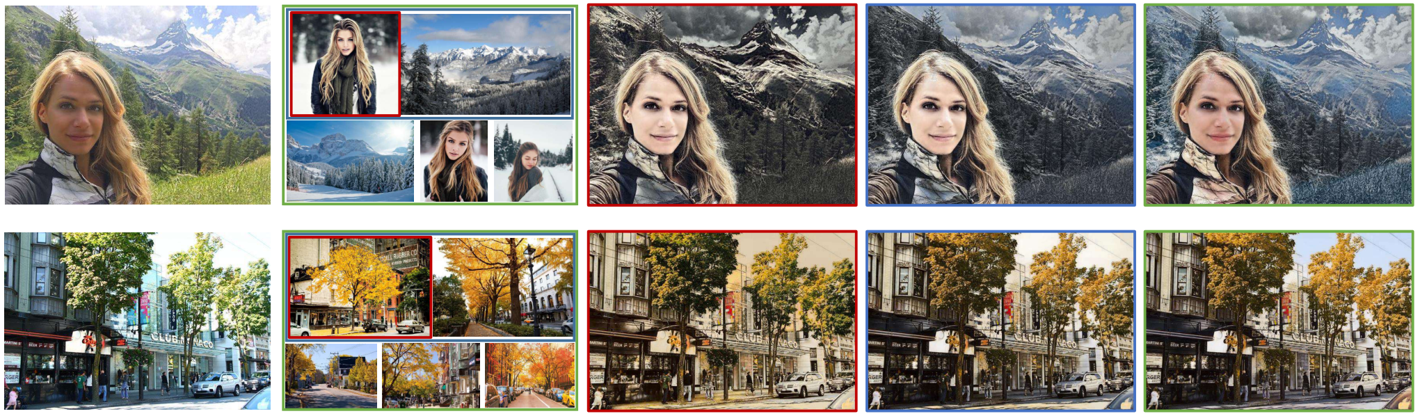
| Source | References | Result (single reference) | Result (two references) | Result (five references) |
Fig. 17(a)(b) demonstrate the average scores and standard deviations of each method. For photorealism and faithfulness, ours and Liao et al. [2017] are ranked 1st ( and ) and 2nd ( and ) respectively, followed by Pitie et al. [2005] ( and ) and Luan et al. [2017] ( and ). The method by Luan et al. [2017] performs worst in photorealism, since it often produces posterization (cartoon-like) effects and introduces unnatural colors; while Pitie et al. [2005] perform the worst in faithfulness to style, since global transfer limits the spatial variety of styles. Fig. 17(c)(d) show the average scores given by every participant. Ours is consistently better than others in both photorealism and faithfulness among all participants. We further conduct repeated-measures ANOVAs on the collected data, and it shows the differences between the four methods from these two aspects are all significant (). We also use simple contrasts to compare each method against our method among all 900 scores in both photorealism and faithfulness (30 participants by 30 scenes). For photorealism, participants prefer ours over Pitie et al. [2005] ( better, equal), Luan et al. [2017] ( better, equal) and Liao et al. [2017] ( better, equal). For faithfulness, participants prefer ours over Pitie et al. [2005] ( better, equal), Luan et al. [2017] ( better, equal) and Liao et al. [2017] ( better, equal).
Since color transfer quality depends on both photorealism and style fidelity, we examine the subject’s preferred result considering both criteria. The pie chart on Fig. 17(e) shows the percentage of each method selected as the best. Our algorithm is the top overall selection over the other three methods at of the time. Fig. 17 (f) gives the detailed numbers of how many times each method is selected as the best in each scene. It shows that more users prefer ours over Pitie et al. [2005] ( vs. ), Luan et al. [2017] ( vs. ), and Liao et al. [2017] ( vs. with equal). Moreover, our method is more efficient than the other two deep network-based methods. The runtime of the four competing algorithms is shown in Table 1.
4.4. Multi-Reference Color Transfer
In all single-reference color transfer methods, reference selection is crucial to achieving satisfactory results. Our method fails to transfer correct colors and yields an unnatural appearance in the regions where no proper color guidance can be found in the reference. This problem can be addressed by introducing multiple references. For example, in the bottom row of Fig. 18, the sky color is incorrect because the single reference does not contain the sky, but it is correct with multiple references, some of which contains the sky. Our multi-reference approach allows the user to provide keywords for controlling the color transfer, for example, “restaurant night” in the first row of 19. “Restaurant” describes the content in the source images, and “night” defines the desired style. To automatically obtain multiple references for the transfer, these keywords are used to retrieve images through a search engine (e.g., Google Images). We collect the top 50 search results as candidates. Naturally, these images may have a wide variety of color styles as well as outliers. To select a set of images with consistent colors, for each candidate image, we compute its normalized histogram in the HSV color space and select the most representative one with a minimum histogram distance to all others. Then we choose the closest subset of images to the representative one as the references for transfer.
Compared with Autostyle [Liu et al., 2014] which uses a global method to transfer vignetting, color, and local contrast from a collection of images searched by a particular keyword for one specific style (e.g., “night”, “beach”, “sunset”), our approach performs a local transfer based on semantic correspondence and thus requires more keywords in order to describe both content and style (e.g., “restaurant night”, “building beach”, “building river sunset”). However, it allows us to produce a more precise color transfer than Autostyle [Liu et al., 2014]. Cycle-GAN [Zhu et al., 2017] also allows the transfer of a specific style (e.g., “winter Yosemite”) to a given source without selecting the reference by leveraging network training on large datasets. Compared to theirs, our method is more flexible when testing different styles without retraining. Our results have fewer checkerboard artifacts, as shown on the bottom two rows of Fig. 19.
 |
 |
 |
 |
| Source | Liu et al. [2014] (“night”) | Refs (“restaurant night”) | Ours |
 |
 |
 |
 |
| Source | Liu et al. [2014] (“beach”) | Refs (“building beach”) | Ours |
 |
 |
 |
 |
| Source | Liu et al. [2014] (“sunset”) | Refs (“building river sunset”) | Ours |
 |
 |
 |
 |
| Source | Zhu et al. [2017] (“winter Yosemite”) | Refs (“Yosemite winter”) | Ours |
 |
 |
 |
 |
| Source | Zhu et al. [2017] (“summer Yosemite”) | Refs (“Yosemite summer”) | Our |
4.5. Colorization
We can also use our method for colorization of gray-scale images. We simply provide color references in the desired style in order to colorize our input gray-scale image. Fig. 20 shows some colorization results.
 |
 |
 |
 |
 |
 |
| Source | Reference | Result | Source | Reference | Result |
5. Concluding Remarks
In this paper, we demonstrate a new algorithm for locally transferring colors across semantically-related images. It not only handles single-reference transfer, but can also be adapted to multi-reference transfer, which avoids the often difficult task of finding a proper reference. We adapt a joint optimization of NNF search and local color transfer across CNN layers in a hierarchical manner. We have shown that our approach is widely applicable to a variety of transfer scenarios in real-world images.
However our method still has limitations. It may mismatch some regions which exist in the source but not in the reference, and thus cause incorrect color transfer, such as the background on the left example of Fig. 21. This often happens in the single-reference transfer and can be reduced by introducing more references. The VGG network we relied on is not trained to distinguish different instances with the same semantic labels, so it may cause color mixing between different instances, such as the man’s shirt on the right example of Fig. 21, which is transfered with mixed blue and white colors from two persons in the reference. A possible improvement would be to train a network on a dataset with instance labels. Moreover, directly applying our image color transfer method to video may cause some flickering artifacts [Chen et al., 2017a]. Addressing this would require temporal constraints, and will be considered for future work. Our color transfer is suitable for semantically similar images. However, it may lead to some unnatural color effects for image pairs without a semantic relationship, such as the yellow water in the failure example. For future work, we would like to explore methods that would allow this example to automatically degenerate to a good color transfer result.
 |
 |
 |
 |
 |
 |
 |
 |
 |
| Source | Reference | Result |
References
- An and Pellacini [2008] Xiaobo An and Fabio Pellacini. 2008. AppProp: all-pairs appearance-space edit propagation. In ACM Transactions on Graphics (TOG), Vol. 27. ACM, 40.
- An and Pellacini [2010] Xiaobo An and Fabio Pellacini. 2010. User-Controllable Color Transfer. In Computer Graphics Forum, Vol. 29. Wiley Online Library, 263–271.
- Arbelot et al. [2017] Benoit Arbelot, Romain Vergne, Thomas Hurtut, and Joëlle Thollot. 2017. Local texture-based color transfer and colorization. Computers & Graphics 62 (2017), 15–27.
- Bae et al. [2006] Soonmin Bae, Sylvain Paris, and Frédo Durand. 2006. Two-scale Tone Management for Photographic Look. ACM Transactions on Graphics (TOG) 25, 3 (2006), 637–645.
- Barnes et al. [2009] Connelly Barnes, Eli Shechtman, Adam Finkelstein, and Dan Goldman. 2009. PatchMatch: A randomized correspondence algorithm for structural image editing. ACM Transactions on Graphics (TOG) 28, 3 (2009), 24.
- Barnes et al. [2010] Connelly Barnes, Eli Shechtman, Dan Goldman, and Adam Finkelstein. 2010. The generalized patchmatch correspondence algorithm. European Conference on Computer Vision (ECCV), 2010 (2010), 29–43.
- Bonneel et al. [2016] Nicolas Bonneel, Gabriel Peyré, and Marco Cuturi. 2016. Wasserstein barycentric coordinates: histogram regression using optimal transport. ACM Transactions on Graphics (TOG) 35, 4 (2016), 71–1.
- Chen et al. [2017a] Dongdong Chen, Jing Liao, Lu Yuan, Nenghai Yu, and Gang Hua. 2017a. Coherent online video style transfer. In Proc. Intl. Conf. Computer Vision (ICCV).
- Chen et al. [2017b] Dongdong Chen, Lu Yuan, Jing Liao, Nenghai Yu, and Gang Hua. 2017b. Stylebank: An explicit representation for neural image style transfer. In Proc. CVPR, Vol. 1. 4.
- Chen et al. [2018b] Dongdong Chen, Lu Yuan, Jing Liao, Nenghai Yu, and Gang Hua. 2018b. Stereoscopic neural style transfer. In Proceedings of the IEEE Conference on Computer Vision and Pattern Recognition, Vol. 10.
- Chen et al. [2018a] Liang-Chieh Chen, George Papandreou, Iasonas Kokkinos, Kevin Murphy, and Alan L Yuille. 2018a. Deeplab: Semantic image segmentation with deep convolutional nets, atrous convolution, and fully connected crfs. IEEE Transactions on Pattern Analysis and Machine Intelligence 40, 4 (2018), 834–848.
- Chen et al. [2013] Xiaowu Chen, Dongqing Zou, Steven Zhiying Zhou, Qinping Zhao, and Ping Tan. 2013. Image matting with local and nonlocal smooth priors. In Computer Vision and Pattern Recognition (CVPR), 2013 IEEE Conference on. 1902–1907.
- Dale et al. [2009] Kevin Dale, Micah K Johnson, Kalyan Sunkavalli, Wojciech Matusik, and Hanspeter Pfister. 2009. Image restoration using online photo collections. In 2009 IEEE International Conference on Computer Vision (ICCV). IEEE, 2217–2224.
- Endo et al. [2016] Yuki Endo, Satoshi Iizuka, Yoshihiro Kanamori, and Jun Mitani. 2016. DeepProp: extracting deep features from a single image for edit propagation. In Computer Graphics Forum, Vol. 35. Wiley Online Library, 189–201.
- Farbman et al. [2008] Zeev Farbman, Raanan Fattal, Dani Lischinski, and Richard Szeliski. 2008. Edge-preserving decompositions for multi-scale tone and detail manipulation. In ACM Transactions on Graphics (TOG), Vol. 27. 67.
- Freedman and Kisilev [2010] Daniel Freedman and Pavel Kisilev. 2010. Object-to-object color transfer: Optimal flows and smsp transformations. In Computer Vision and Pattern Recognition (CVPR), 2010 IEEE Conference on. IEEE, 287–294.
- Gatys et al. [2015] Leon A Gatys, Alexander S Ecker, and Matthias Bethge. 2015. A neural algorithm of artistic style. CoRR abs/1508.06576 (2015).
- HaCohen et al. [2011] Yoav HaCohen, Eli Shechtman, Dan B Goldman, and Dani Lischinski. 2011. Non-rigid dense correspondence with applications for image enhancement. ACM transactions on graphics (TOG) 30, 4 (2011), 70.
- He et al. [2018] Mingming He, Dongdong Chen, Jing Liao, Pedro V. Sander, and Lu Yuan. 2018. Deep Exemplar-based Colorization. ACM Transactions on Graphics (TOG) 37, 4 (2018), 110.
- Hertzmann et al. [2001] Aaron Hertzmann, Charles E Jacobs, Nuria Oliver, Brian Curless, and David H Salesin. 2001. Image analogies. In Proceedings of the 28th annual conference on Computer graphics and interactive techniques. ACM, 327–340.
- Hristova et al. [2015] Hristina Hristova, Olivier Le Meur, Rémi Cozot, and Kadi Bouatouch. 2015. Style-aware robust color transfer. In Proceedings of the workshop on Computational Aesthetics. Eurographics Association, 67–77.
- Iizuka et al. [2016] Satoshi Iizuka, Edgar Simo-Serra, and Hiroshi Ishikawa. 2016. Let there be color!: joint end-to-end learning of global and local image priors for automatic image colorization with simultaneous classification. ACM Transactions on Graphics (TOG) 35, 4 (2016), 110.
- Isola et al. [2017] Phillip Isola, Jun-Yan Zhu, Tinghui Zhou, and Alexei A Efros. 2017. Image-to-image translation with conditional adversarial networks. (2017), 5967–5976.
- Khan et al. [2017] Asad Khan, Luo Jiang, Wei Li, and Ligang Liu. 2017. Fast color transfer from multiple images. Applied Mathematics-A Journal of Chinese Universities 32, 2 (2017), 183–200.
- Kolmogorov and Zabin [2004] Vladimir Kolmogorov and Ramin Zabin. 2004. What energy functions can be minimized via graph cuts? IEEE transactions on pattern analysis and machine intelligence 26, 2 (2004), 147–159.
- Laffont et al. [2014] Pierre-Yves Laffont, Zhile Ren, Xiaofeng Tao, Chao Qian, and James Hays. 2014. Transient attributes for high-level understanding and editing of outdoor scenes. ACM Transactions on Graphics (TOG) 33, 4 (2014), 149.
- Lee et al. [2016] Joon-Young Lee, Kalyan Sunkavalli, Zhe Lin, Xiaohui Shen, and In So Kweon. 2016. Automatic content-aware color and tone stylization. In Computer Vision and Pattern Recognition (CVPR), 2016 IEEE Conference on. 2470–2478.
- Levin et al. [2004] Anat Levin, Dani Lischinski, and Yair Weiss. 2004. Colorization using optimization. In ACM transactions on graphics (TOG), Vol. 23. ACM, 689–694.
- Levin et al. [2008] Anat Levin, Dani Lischinski, and Yair Weiss. 2008. A closed-form solution to natural image matting. IEEE Transactions on Pattern Analysis and Machine Intelligence 30, 2 (2008), 228–242.
- Li and Wand [2016] Chuan Li and Michael Wand. 2016. Combining markov random fields and convolutional neural networks for image synthesis. In Computer Vision and Pattern Recognition (CVPR), 2016 IEEE Conference on. 2479–2486.
- Liao et al. [2017] Jing Liao, Yuan Yao, Lu Yuan, Gang Hua, and Sing Bing Kang. 2017. Visual Attribute Transfer Through Deep Image Analogy. ACM Transactions on Graphics (TOG) 36, 4 (2017), 120:1–120:15.
- Lischinski et al. [2006] Dani Lischinski, Zeev Farbman, Matt Uyttendaele, and Richard Szeliski. 2006. Interactive local adjustment of tonal values. In ACM Transactions on Graphics (TOG), Vol. 25. ACM, 646–653.
- Liu et al. [2014] Yiming Liu, Michael Cohen, Matt Uyttendaele, and Szymon Rusinkiewicz. 2014. Autostyle: Automatic style transfer from image collections to users’ images. In Computer Graphics Forum, Vol. 33. Wiley Online Library, 21–31.
- Luan et al. [2017] Fujun Luan, Sylvain Paris, Eli Shechtman, and Kavita Bala. 2017. Deep Photo Style Transfer. (2017), 6997–7005.
- Mechrez et al. [2017] Roey Mechrez, Eli Shechtman, and Lihi Zelnik-Manor. 2017. Photorealistic Style Transfer with Screened Poisson Equation. CoRR abs/1709.09828 (2017).
- Odena et al. [2016] Augustus Odena, Vincent Dumoulin, and Chris Olah. 2016. Deconvolution and Checkerboard Artifacts. Distill (2016). http://distill.pub/2016/deconv-checkerboard
- Pitie et al. [2005] Francois Pitie, Anil C Kokaram, and Rozenn Dahyot. 2005. N-dimensional probability density function transfer and its application to color transfer. In 2005 IEEE International Conference on Computer Vision (ICCV), Vol. 2. IEEE, 1434–1439.
- Reinhard et al. [2001] Erik Reinhard, Michael Adhikhmin, Bruce Gooch, and Peter Shirley. 2001. Color transfer between images. IEEE Computer graphics and applications 21, 5 (2001), 34–41.
- Roweis and Saul [2000] Sam T Roweis and Lawrence K Saul. 2000. Nonlinear dimensionality reduction by locally linear embedding. science 290, 5500 (2000), 2323–2326.
- Russakovsky et al. [2015] Olga Russakovsky, Jia Deng, Hao Su, Jonathan Krause, Sanjeev Satheesh, Sean Ma, Zhiheng Huang, Andrej Karpathy, Aditya Khosla, Michael Bernstein, et al. 2015. Imagenet large scale visual recognition challenge. International Journal of Computer Vision 115, 3 (2015), 211–252.
- Shen et al. [2016] Xiaoyong Shen, Xin Tao, Chao Zhou, Hongyun Gao, and Jiaya Jia. 2016. Regional foremost matching for internet scene images. ACM Transactions on Graphics (TOG) 35, 6 (2016), 178.
- Shih et al. [2014] YiChang Shih, Sylvain Paris, Connelly Barnes, William T. Freeman, and Frédo Durand. 2014. Style Transfer for Headshot Portraits. ACM Transactions on Graphics (TOG) 33, 4 (2014), 148:1–148:14.
- Shih et al. [2013] Yichang Shih, Sylvain Paris, Frédo Durand, and William T Freeman. 2013. Data-driven hallucination of different times of day from a single outdoor photo. ACM Transactions on Graphics (TOG) 32, 6 (2013).
- Simakov et al. [2008] Denis Simakov, Yaron Caspi, Eli Shechtman, and Michal Irani. 2008. Summarizing visual data using bidirectional similarity. In Computer Vision and Pattern Recognition (CVPR), 2008 IEEE Conference on. IEEE, 1–8.
- Simonyan and Zisserman [2014] Karen Simonyan and Andrew Zisserman. 2014. Very deep convolutional networks for large-scale image recognition. CoRR abs/1409.1556 (2014).
- Sunkavalli et al. [2010] Kalyan Sunkavalli, Micah K. Johnson, Wojciech Matusik, and Hanspeter Pfister. 2010. Multi-scale Image Harmonization. ACM Transactions on Graphics (TOG) 29, 4 (2010), 125:1–125:10.
- Tai et al. [2005] Yu-Wing Tai, Jiaya Jia, and Chi-Keung Tang. 2005. Local color transfer via probabilistic segmentation by expectation-maximization. In Computer Vision and Pattern Recognition (CVPR), 2005 IEEE Conference on, Vol. 1. IEEE, 747–754.
- Tong et al. [2007] Wai-Shun Tong, Chi-Keung Tang, Michael S Brown, and Ying-Qing Xu. 2007. Example-based cosmetic transfer. In Computer Graphics and Applications, 2007. PG’07. 15th Pacific Conference on. IEEE, 211–218.
- Welsh et al. [2002] Tomihisa Welsh, Michael Ashikhmin, and Klaus Mueller. 2002. Transferring color to greyscale images. In ACM Transactions on Graphics (TOG), Vol. 21. ACM, 277–280.
- Yan et al. [2016] Zhicheng Yan, Hao Zhang, Baoyuan Wang, Sylvain Paris, and Yizhou Yu. 2016. Automatic photo adjustment using deep neural networks. ACM Transactions on Graphics (TOG) 35, 2 (2016), 11.
- Yoo et al. [2013] Jae-Doug Yoo, Min-Ki Park, Ji-Ho Cho, and Kwan H Lee. 2013. Local color transfer between images using dominant colors. Journal of Electronic Imaging 22, 3 (2013), 033003–033003.
- Zhang et al. [2016] Richard Zhang, Phillip Isola, and Alexei A Efros. 2016. Colorful image colorization. In European Conference on Computer Vision (ECCV), 2016. Springer, 649–666.
- Zhao et al. [2012] Qi Zhao, Ping Tan, Qiang Dai, Li Shen, Enhua Wu, and Stephen Lin. 2012. A closed-form solution to retinex with nonlocal texture constraints. IEEE transactions on pattern analysis and machine intelligence 34, 7 (2012), 1437–1444.
- Zhu et al. [2017] Jun-Yan Zhu, Taesung Park, Phillip Isola, and Alexei A Efros. 2017. Unpaired Image-to-Image Translation using Cycle-Consistent Adversarial Networks. (2017), 2242–2251.