Elastic-Net: Boosting Energy Efficiency and Resource Utilization in 5G C-RANs
Abstract
Current Distributed Radio Access Networks (D-RANs), which are characterized by a static configuration and deployment of Base Stations (BSs), have exposed their limitations in handling the temporal and geographical fluctuations of capacity demands. At the same time, each BS’s spectrum and computing resources are only used by the active users in the cell range, causing idle BSs in some areas/times and overloaded BSs in other areas/times. Recently, Cloud Radio Access Network (C-RAN) has been introduced as a new centralized paradigm for wireless cellular networks in which—through virtualization—the BSs are physically decoupled into Virtual Base Stations (VBSs) and Remote Radio Heads (RRHs). In this paper, a novel elastic framework aimed at fully exploiting the potential of C-RAN is proposed, which is able to adapt to the fluctuation in capacity demand while at the same time maximizing the energy efficiency and resource utilization. Simulation and testbed experiment results are presented to illustrate the performance gains of the proposed elastic solution against the current static deployment.
Index Terms:
Cloud Radio Access Network; Virtual Base Station; Energy Efficiency; Resource Utilization.I Introduction
Motivation: Over the last few years, proliferation of personal mobile computing devices like tablets and smartphones along with a plethora of data-intensive mobile applications has resulted in a tremendous increase in demand for ubiquitous and high data rate wireless communications. The current practice to enhance the spectral efficiency and data rate is to increase the number of Base Stations (BSs) and go for smaller cells so as to increase the band reuse factor. However, it is studied that increasing the BS density or the number of transmit antennas will decrease the energy efficiency due to the dynamic traffic variation [1]. The number of active users at different locations varies depending on the time of the day and week. This movement of mobile network load based on time of the day/week is referred to as the “tidal effect”. In the traditional Distributed Radio Access Network (D-RAN), each BS’s spectrum and computing resources are only used by the active users in the cell range. Hence, deploying small cells for the peak (worst case) traffic time leads to grossly under-utilized BSs in some areas/times and is highly energy inefficient, while deploying cell for the average traffic time leads to oversubscribed BSs in some other areas/times.
At the stage of network planning, cell size and capacity are usually determined based on the estimation of peak traffic load. However, due to the tidal effect, there are no fixed cell size and transmission power that optimize the overall power consumption of the network. This means that the use of small cells is quite efficient in terms of power consumption as well as utilization of spectrum and computing resources when the capacity demand is high and evenly distributed in space; however, it becomes less so when the data traffic is low and/or uneven due to the static resource provisioning and fixed BS power consumptions. On the other hand, the economic impact of power consumption is particularly dire in emerging markets and the Fifth Generation (5G) of wireless networks must be not only spectral efficient but also energy efficient (e.g., a 1000 improvement in energy efficiency is expected by 2020). Although several recent efforts have been made to increase spectral efficiency [2] and to reduce the power consumption of existing small cell networks, limited attention has been given towards optimizing the overall network deployment. Hence, a novel design and architecture is necessary for the next generation of wireless network to overcome these challenges.
A New Centralized Cellular Network Paradigm: Cloud Radio Access Network (C-RAN) [3] is a new architecture for the next generation of wireless cellular networks that allows for a dynamic reconfiguration of spectrum/computing resources (Fig. 1). C-RAN consists of three parts: 1) Remote Radio Heads (RRHs) plus antennae, which are located at the remote site and are controlled by Virtual Base Stations (VBSs) housed in a centralized processing pool, 2) the Base Band Unit (BBU) (known as VBS pool) composed of high-speed programmable processors and real-time virtualization technology to carry out the digital processing tasks, and 3) low-latency high-bandwidth optical fibers, which connect the RRHs to the VBS pool. The communication functionalities of the VBSs are implemented on Virtual Machines (VMs), which are housed in one or more racks of a small cloud datacenter. This centralized characteristic along with virtualization technology and low-cost relay-like RRHs provides a higher degree of freedom to make optimized decisions, and has made C-RAN a promising candidate to be incorporated into the 5G networks [4, 5, 6, 7].
Our Contributions: In this paper, we focus on optimizing the power consumption and resource utilization by leveraging the full potential of the C-RAN architecture. We propose a novel elastic resource provisioning framework, called ‘‘Elastic-Net’’, to minimize the power consumption while addressing the fluctuations in per-user capacity demand. In our solution, we divide the covered region of the network into clusters based on the traffic model and, within each cluster, we dynamically adapt the active RRH density, transmission power, and size of the VM11 1 The size of a VM is represented in terms of its processing power, memory and storage capacity, and network interface speed. based on the traffic fluctuations so as to minimize the power consumption while maximizing the resource utilization. To minimize the power consumption in the cell sites while ensuring a certain minimum coverage and data rate, we propose to dynamically optimize and adapt the RRH density and transmission power based on the traffic demand and user density. Likewise, to minimize the power consumption in the cloud we dynamically optimize and adapt the size of the VMs while ensuring that the frame-processing deadline is met.
II System Model
We consider a C-RAN downlink system and assume that each user is served by the nearest active RRH. The RRHs and users are distributed according to two independent Poisson Point Processes (PPPs) in , denoted as and , respectively. Let and denote the RRH density and the time-dependent user density, respectively. The set of all RRHs is denoted by , where is the set of active RRHs and is the set of inactive RRHs (). Let also denote the RRH activity factor, which indicates the ratio of active RRHs to all RRHs, where is the time-dependent density of active RRHs. The total bandwidth is denoted by and the bandwidth per user is given by .
 |
 |
| (a) Day | (b) Night |
RRH and Transport Network Power Consumption Model: Since in C-RAN the BSs are decoupled into RRHs and VBSs, we divide the network power consumption into two parts: (i) RRH and transport network power consumption and (ii) VBS pool power consumption. For the power consumption of a RRH, we consider a linear model as in [8],
| (1) |
where is the active circuit power consumption, is the power amplifier efficiency, is the transmission power, and is the RRH power consumption in the sleep mode. We also consider the future Passive Optical Network (PON) to provide low-cost, high-bandwidth, low-latency connections between the RRHs and VBS pool [9]. PON comprises an Optical Line Terminal (OLT) that resides in the VBS pool and connects a set of associated Optical Network Units (ONUs) through a single fiber. In this paper, we consider fast/cyclic sleep mode where the ONU state alternates between the active state (when the RRH is in the active state) and the sleep state (when the RRH is in the sleep state). Hence, the power consumption of the transport network is given as in [9],
| (2) |
where is the OLT power consumption in the VBS pool and is the ONU power consumption, given as,
| (3) |
where and are the consumed power by each ONU in the active and sleep mode, respectively. Since is consumed in the VBS pool, we consider it in the power consumption of the VBS pool. Therefor, the overall area RRH and transport network power consumption is given by,
| (4) |
VBS Pool Power Consumption Model: As discussed in [10], compared to other system resources, the CPU consumes the main part of the power in the VBS pool; hence, in this work, we focus on minimizing its power consumption. In order to model the power consumption of the VBS pool, we introduce the notion of size of a VM, which is represented in terms of its processing power [CPU cycles per second]; for each VM, we consider the power model defined as,
| (5) |
where is the size of the VM in terms of CPU cycles per second, is the maximum power consumed per unit VM size when the server is fully utilized, is the fraction of power consumed by the idle VM, and is VM utilization. Note that, in our model, and change over time due to the workload variation and hence they are functions of time.
III Elastic-Net: Demand-Aware Provisioning
In our solution, as depicted in Fig. 1, we cluster the neighboring RRHs and their corresponding VBSs based on traffic model, and in each cluster we adapt the system parameters accordingly. We advocate demand-aware resource provisioning where in each cluster the active RRH density, transmission power, and size of the VM are dynamically changed over time to minimize the power consumption and to meet the fluctuating traffic demand as well as network constraints. For instance, as shown in Fig. 1(a)-(b), due to the higher capacity demand during day time in cluster #2 (a), we provision it with more active RRH and higher size of VBS-Cluster rather than during night time (b), when we have less capacity demand. Hence, our objective is to obtain the optimal active RRH density, transmission power, and size of VM for each cluster so that the power consumption is minimized while meeting a predefined coverage probability, per-user data rate, and frame-processing time. Our optimization problem for the cluster can be cast as,
| (6a) | ||||||
| subject to | (6b) | |||||
| (6c) | ||||||
| (6d) | ||||||
where and are the area power consumption and VBS-Cluster power consumption of the cluster, respectively, is the coverage probability at no noise regime, is the per-user minimum data rate, is the frame-processing time, is frame deadline, and is a positive number in . , , and are also the RRH activity factor, transmission power, and size of the VM for the cluster, respectively. Due to the temporal variation of traffic demand in each cluster, , , and are time dependent; hence, the optimal solution in general varies over time.
The density of active and inactive RRHs in the are,
| (7a) | ||||
| (7b) | ||||
where is the density of all RRHs in the cluster. By substituting (7a) and (7b) into (4), we can write,
| (8) |
where
| (9a) | ||||
| (9b) | ||||
From (8) and (9a), we see that the objective function is non-convex because of the multiplication term of and . To minimize the objective function, as in [11], we can use the coordinate descent algorithm and minimize , , and independently.
III-A Optimal Active RRH Density
Lemma 1.
The minimum RRH activity factor for which the constraint is met is given by,
| (10) |
where
| (11) |
Proof.
The spectral efficiency achievable by a randomly chosen user when it is in coverage is given as in [12],
| (12) |
Hence, the per-user data rate in the cluster and at time instant can be written as,
| (13) |
So, considering constraint (6c), we can write,
| (14) |
which establishes the minimum RRH activity factor as a function of to satisfy the per-user data-rate constraint. ∎
III-B Optimal Transmission Power
Given a fixed active RRH density, we can minimize the transmit power of the active RRHs so as to achieve a certain coverage and outage probability. Since in our solution the active RRH density of different clusters changes over time based on the traffic demand, we need to also dynamically optimize the transmit power accordingly. This can further decrease the power consumption of the system. For instance, when the density of active RRHs becomes higher, each RRH has only a small coverage area and users can be in coverage even with a lower transmission power.
Lemma 2.
The minimum transmission power for which the constraint is met is given by,
| (15) |
where
| (16a) | ||||
| (16b) | ||||
Proof.
The coverage probability in the cluster is given as [13],
| (17) |
Now, by using the substitution in (17) and the approximation (in the case of low-noise regimes, i.e., ), we can write,
| (18) |
where is the coverage probability without noise [13], i.e.,
| (19) |
and is the standard gamma function. The minimum transmission power that satisfies the coverage constraints is obtained by combining (18) and (6b). ∎
III-C Optimal Size of VM
We recast the power consumption of the VBS-Cluster,
| (20) |
where, for a given workload, is inversely proportional to [14]. So, to minimize the power consumption of the VM, we need to minimize the size of the VM (CPU cores) such that the network requirements are met. The workload in the VBS-Cluster depends on the LTE MCS index, number of PRBs, and the channel bandwidth. Moreover, according to [15], the Round Trip Time (RTT) between RRH and VBS pool cannot exceed . Since the total delay budget in LTE is considered as , this leaves the VBS-Cluster with only about for signal processing. For this matter, we consider a modified model of the processing time presented in [16], which is given by,
| (21) |
where is the processing time and is measured in , is the number of PRBs, is a MSC-dependent constant, is the number of dedicated CPU cores to the VBS-Cluster, and is the CPU speed measured in . Hence, the minimum number of required CPU cores to meet the frame deadline is given by,
| (22) |
where is the frame deadline.
| Parameters | Mode/Value |
|---|---|
| Cellular Layout | Homogeneous Poisson Point Process |
| Channel Model | Path Loss and Shadowing |
| Channel Bandwidth | |
| Number of Antennas | |
| OLT power consumption () | |
| ONU Power Consumption in Active Mode () | |
| ONU Power Consumption in Sleep Mode () | |
| RRH Circuit Power Consumption in Active Mode () | |
| RRH power consumption in sleep mode () | |
| Maximum power consumed per each CPU core () | |
| Power Amplifier Efficiency () | |
| MSC Dependent Constant () | |
| Fraction of Power Consumed by Idle VBS () | |
| Fraction of Minimum Coverage Probability () | |
| Minimum Data Rate () |
IV Performance Evaluation
In this section, we provide a range of simulations and real-time emulations to evaluate the performance of our solution. In the simulations, we consider a cellular network where the RRHs and the users are distributed according to two independent homogeneous PPPs. Table I lists the stimulation parameters used during our experiments.
 |
 |
 |
 |
| (a) | (b) | (c) | (d) |
In order to show the performance of our dynamic solution, we simulate the traffic fluctuation on a typical operational day and show how Elastic-Net dynamically adapts the RRH density, transmission power, and size of VBS-Clusters to minimize the power consumption while at the same time meeting the network constraints. As shown in Fig. 1, we consider a network with clusters where each cluster covers an area of km2 and has its own traffic and user density fluctuation.
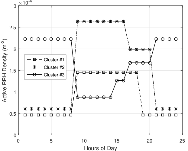
As shown in Fig. 2(a), clusters #1 and #2 (corresponding to the downtown and entertainment areas, respectively) have lower user density on early morning and late night, while cluster #3 (residential area) has higher user density at those times. Figure 2(b) illustrates the minimum active RRH density adaptation required to serve the corresponding user density fluctuation in different clusters. As expected, the RRH density fluctuation corresponds to the user density fluctuation. This means that for the high traffic demand times we need a higher number of active RRHs and smaller cells. The time varying transmission power for different clusters is shown in Fig. 2(c). It is clear that for the peak traffic times we need a lower transmission power than in low traffic times. This is because in the peak traffic times we have higher active RRH density and, consequently, the coverage area of each RRH becomes smaller. Figure 2(d) also shows the power consumption of VBS-Clusters in the VBS pool.
In Figs. 3(a-c), we compare the traditional static provisioning against Elastic-Net. As shown in (a), (b), and (c), depending on the traffic fluctuation there is a noticeable difference between the power consumption of Elastic-Net and Static-Net. For instance, in cluster #1 and for low traffic times (7 PM–8 AM) we have decrease in power consumption by Elastic-Net. However, for the peak traffic times (8 AM–7 PM), we have only decrease in power consumption. This confirms our statements in Sect. I that a small-cell deployment is efficient when the capacity demand or user density is high, while it becomes less so when the traffic demand is low.
 |
 |
 |
| (a) | (b) | (c) |
V Conclusion
In the context of C-RAN—a new centralized paradigm for wireless cellular networks in which the Base Stations (BSs) are physically decoupled into Virtual Base Stations (VBSs) and Remote Radio Heads (RRHs)—we proposed a novel demand-aware reconfigurable solution, named Elastic-Net, to minimize the network power consumption and to adapt to the fluctuations in per-user capacity demand. We divided the covered region of the cellular network into clusters based on active traffic, and dynamically adjusted RRH density, transmission power, and size of the Virtual Machine (VM) holding the VBS so that the network power consumption is minimized and the network constraints are met. Simulation results corroborated our analysis and confirmed the benefits of our solution.
Acknowledgment: This work was supported in part by the National Science Foundation Grant No. CNS-1319945.
References
- [1] C. Li, J. Zhang, and K. Letaief, “Throughput and energy efficiency analysis of small cell networks with multi-antenna base stations,” IEEE Trans. Wireless Commun., vol. 13, no. 5, pp. 2505–2517, 2013.
- [2] M. Hajimirsadeghi, G. Sridharan, W. Saad, and N. B. Mandayam, “Inter-network dynamic spectrum allocation via a colonel blotto game,” in Proc. IEEE CISS, 2016, pp. 252–257.
- [3] C. M. R. Institute, “C-RAN: The Road Towards Green RAN,” in C-RAN International Workshop, Oct. 2011.
- [4] T. X. Tran, A. Hajisami, and D. Pompili, “QuaRo: A queue-aware robust coordinated transmission strategy for downlink C-RANs,” in Proc. IEEE SECON, 2016, pp. 1–9.
- [5] A. Hajisami and D. Pompili, “Dynamic joint processing: Achieving high spectral efficiency in uplink 5g cellular networks,” Computer Networks, vol. 126, pp. 44–56, 2017.
- [6] A. Hajisami, H. Viswanathan, and D. Pompili, ““Cocktail Party in the Cloud”: Blind Source Separation for Co-operative Cellular Communication in Cloud RAN,” IEEE International Conference on Mobile Ad hoc and Sensor Systems (MASS), pp. 37–45, 2014.
- [7] M. Hajimirsadeghi, N. B. Mandayam, and A. Reznik, “Joint caching and pricing strategies for popular content in information centric networks,” IEEE Journal on Selected Areas in Communications, vol. 35, no. 3, pp. 654–667, 2017.
- [8] G. Auer, V. Giannini, C. Desset et al., “How much energy is needed to run a wireless network?” IEEE Wireless Commun., vol. 18, no. 5, pp. 40–49, 2011.
- [9] A. R. Dhaini, P.-H. Ho, G. Shen, and B. Shihada, “Energy efficiency in tdma-based next-generation passive optical access networks,” IEEE/ACM Trans. Netw. (TON), vol. 22, no. 3, pp. 850–863, 2014.
- [10] A. Beloglazov, J. Abawajy, and R. Buyya, “Energy-aware resource allocation heuristics for efficient management of data centers for cloud computing,” Future Generation Computer Systems, vol. 28, no. 5, pp. 755–768, 2012.
- [11] K. Lin, J. Xu, I. M. Baytas, S. Ji, and J. Zhou, “Multi-task feature interaction learning,” in Proc. ACM Int. Conf. Knowledge Discovery and Data Mining, 2016, pp. 1735–1744.
- [12] H. S. Dhillon, R. K. Ganti, F. Baccelli, and J. G. Andrews, “Modeling and analysis of k-tier downlink heterogeneous cellular networks,” IEEE J. Sel. Areas Commun. (JSAC), vol. 30, no. 3, pp. 550–560, 2012.
- [13] J. G. Andrews, F. Baccelli, and R. K. Ganti, “A tractable approach to coverage and rate in cellular networks,” IEEE Trans. Commun., vol. 59, no. 11, pp. 3122–3134, 2011.
- [14] K. S. Trivedi, R. A. Wagner, and T. M. Sigmon, “Optimal selection of cpu speed, device capacities, and file assignments,” Journal of the ACM (JACM), vol. 27, no. 3, pp. 457–473, Jul. 1980.
- [15] P. Chanclou, A. Pizzinat, F. Le Clech, T. Reedeker, Y. Lagadec, F. Saliou, B. Le Guyader, L. Guillo, Q. Deniel, and S. Gosselin, “Optical fiber solution for mobile fronthaul to achieve cloud radio access network,” in Proc. IEEE Future Network and Mobile Summit, 2013, pp. 1–11.
- [16] I. Alyafawi, E. Schiller, T. Braun, D. Dimitrova, A. Gomes, and N. Nikaein, “Critical issues of centralized and cloudified lte-fdd radio access networks,” IEEE ICC, pp. 5523–5528, 2015.