Redefining A in RGBA: Towards a Standard for Graphical 3D Printing
Abstract.
Advances in multimaterial 3D printing have the potential to reproduce various visual appearance attributes of an object in addition to its shape. Since many existing 3D file formats encode color and translucency by RGBA textures mapped to 3D shapes, RGBA information is particularly important for practical applications. In contrast to color (encoded by RGB), which is specified by the object’s reflectance, selected viewing conditions and a standard observer, translucency (encoded by A) is neither linked to any measurable physical nor perceptual quantity. Thus, reproducing translucency encoded by A is open for interpretation.
In this paper, we propose a rigorous definition for A suitable for use in graphical 3D printing, which is independent of the 3D printing hardware and software, and which links both optical material properties and perceptual uniformity for human observers. By deriving our definition from the absorption and scattering coefficients of virtual homogenous reference materials with an isotropic phase function, we achieve two important properties. First, a simple adjustment of A is possible, which preserves the translucency appearance if an object is rescaled for printing. Second, determining the value of A for a real (potentially non-homogenous) material, can be achieved by minimizing a distance function between light transport measurements of this material and simulated measurements of the reference materials. Such measurements can be conducted by commercial spectrophotometers used in graphic arts.
Finally, we conduct visual experiments employing the method of constant stimuli, and derive from them an embedding of A into a nearly perceptually-uniform scale of translucency for the reference materials.
Keywords:
3D printing, metamerism, translucency1. Introduction
Advances in 3D printing allow the combination of multiple printing materials with different optical properties into a single object at a very high resolution. This allows the reproduction of not only the object’s shape but also its visual appearance attributes such as color (Brunton et al., 2015), translucency (Hašan et al., 2010; Dong et al., 2010) or gloss (Baar et al., 2014).
Many existing 3D file formats encode spatially-resolved information of (albedo) color and opacity of an object as a RGBA texture mapped to its 3D geometry. This information is widely used in rendering, where the RGB color information is typically interpreted as device-independent standard RGB (Süsstrunk et al., 1999) and (also called channel) as a blending or mixing parameter to produce transparent overlays in image composition assuming additive color mixture (Porter and Duff, 1984). Such an interpretation is common for 3D file formats, including the 3MF format, which is being pushed by many industry players as a standard for 3D printing: In the core specification (3MF Consortium, 2015a) the interpretation of is left unspecified, whereas in the materials and properties extension (3MF Consortium, 2015b) additive blending is specified, which however also stipulates that the first color layer must be opaque. Thus, translucent objects are not possible at all according to this interpretation; it is purely a mechanism for additively mixing colors in a specified order.
Using an additive color mixture model is simple, computationally efficient and robust for on-screen display, but it has severe shortcomings (Faul, 2017): light is altered by matter subtractively not additively, i.e. many real transparent materials cannot be described by this interpretation. As a result, renderings employing as an additive mixture parameter are suitable for illustrative purposes rather than accurately simulating the appearance of real objects.
Nonetheless, it is highly desirable to capture perceived translucency of real objects within a single parameter, foremost because it allows the seamless continued use of existing image and 3D file formats, it is supported by various existing 3D design and image manipulation tools, but also because the perceptual dimension of translucency is known to be small (Gkioulekas et al., 2013). Therefore, in this paper we present a new interpretation of the channel in RGBA for use in graphical 3D printing aiming to encode a significant portion of perceived translucency information.
For the purpose of reproducing translucent objects by 3D printing, a few properties of are desired:
- (1)
must be linked to a measurable quantity. Only then, can be assigned to real materials via measurements and print material arrangements can be adjusted to match this quantity.
- (2)
For print reproductions, a perceptually uniform scale for is important, allowing the minimization of perceived errors rather than physical ones. The viewing condition for this scale must agree with the RGB conditions to ensure consistency of color and translucency. In color printing, the viewing/illuminating geometry (side-lighting) is specified by the International Color Consortium (ICC, 2010) and is supported by color and spectrophotometric measurement devices employed in graphic arts (ISO13655, 2009), which are used to calibrate the printers. This rules out backlighting conditions for specifying the perceptual scale, even though the translucency for materials possessing complex light transport properties may appear different for side- and backlighting conditions (Xiao et al., 2014).
- (3)
If an object made of a translucent material is scaled (most commonly shrunk) for printing, it is desirable that average light transport distances can be adjusted accordingly to preserve perceptual translucency cues. Therefore, should be adjustable to the print size in relation to the original object size in an intuitive, predictable and computationally efficient way.
- (4)
For design purposes, the absence of cross-contamination between the chromatic channels (chroma and hue) and is important, i.e. that changing the chromatic channels has no effect on perceived translucency and vice versa, for the specified viewing conditions. Predictors for chroma and hue can be computed by transforming standard RGB color spaces to the CIELCh color space, CIECAM02 (CIE Publication No. 159, 2004) or LAB2000HL (Lissner and Urban, 2012).
Given these observations and constraints, this paper makes the following two main contributions:
- (1)
A definition of based on a set of virtual reference materials and a measurement methodology for extracting BSSRDF information impacting perceptual translucency cues from real and simulated measurements. This definition allows adjusting to the print size so that the print has perceptually similar translucency as the original model.
- (2)
Determining a psychometric function allows us to adjust the definition of to be nearly perceptually uniform.
By contrast, this paper does not propose a 3D printing pipeline for fabricating translucent objects. Our goal is to provide a definition that is both physically and perceptually meaningful, compatible with existing data formats, practically measurable for both real materials and 3D printed characterization targets, while remaining as neutral as possible concerning 3D printing hardware and software, thus making it applicable as a device independent standard for 3D printing systems capable of reproducing varying degrees of translucency. To illustrate the practicality and expressiveness of our definition, in Section 6 and Appendix F we show some 3D printed examples generated using a recently proposed color and translucency 3D printing pipeline (Brunton et al., 2018).
1.1. Background
Light reflectance and scattering properties of a non-fluorescent homogenous material are described by the 8-dimensional Bidirectional Surface Scattering Reflectance Distribution Function (BSSRDF). It is the ratio of outgoing radiance and incident flux computed for any bidirectional geometry of incoming and outgoing light rays. There exist candidate representations for graphical 3D printing based on approximations or simplifications of the full BSSRDF by factoring the complete function into distinct physical phenomena. Jensen et al. presented a 10-parameter model (2001). The SubEdit model (Song et al., 2009) uses 1D scattering profiles to approximate diffuse scattering, and allows interactive rendering and editing of subsurface scattering; examples were shown with a 24-dimensional variant. This representation has even been used in fabrication pipelines (Dong et al., 2010; Hašan et al., 2010). Spatially-varying versions of these representations require either high-dimensional texture or multiple textures mapped onto the surface geometry. More importantly, neither considers human perception of translucency as is done for color, but rather approximate the underlying physical phenomena.
A BSSRDF allows us to compute stimuli yielding CIEXYZ and standard RGB color space values (Süsstrunk et al., 1999) for any measurement geometry. In printing, a circular 45/0 measurement geometry is used and supported by many spectrophotometers (ISO13655, 2009), i.e. the surface is circularly illuminated under to its normal and the stimulus is measured at . Thus, a material’s RGB values contain only a small portion of the BSSRDF information selected already by the measurement geometry.
Analogously, our strategy to define is to identify relevant BSSRDF information causing a material to appear more or less translucent. Fleming and Bülthoff concluded from visual matching experiments of simulated translucent objects that the “physics of translucency is simply too complex for the visual system to run the generative equations in reverse and estimate intrinsic physical parameters via inverse optics … instead the visual system relies on simple image heuristics [cues] that correlate with translucency" (Fleming and Bülthoff, 2005). They have also investigated the impact of color on perceived translucency and came to the conclusion that “the saturation component is neither necessary nor sufficient to yield an impression of translucency". This is a good reason to keep independent of chroma and hue. We note that later investigations (Xiao et al., 2012) suggested, qualitatively, that chromatic components may have an impact on translucency perception. Given the lack of quantitative results concerning this, we leave consideration of this for future work.
Gkioulekas et al. evaluated the impact of the phase function on the appearance of translucent materials (2013). The phase function describes the scattering-induced distribution of light within a material and in addition to the absorption and scattering coefficient it is one parameter of the Radiative Transfer Equation (Chandrasekhar, 1960) that describes light transport within materials. By linearly combining the Henyey-Greenstein (HG) and von Mises-Fisher (vMF) lobes, they created a family of phase functions that significantly extends the often used HG model. They showed by conducting extensive paired-comparison experiments on rendered objects and multidimensional scaling that the physical parameter space can be embedded into a two-dimensional meaningful appearance space. The two-dimensional embedding is robust against variations in the object’s shape, scattering coefficient and lighting variations and indicates that translucency perception is low dimensional even though the family of investigated phase functions is likely not complete as stated by the authors.
Motoyoshi (2010) investigated visual translucency cues by two visual experiments on computer simulated objects. He suggests that a robust cue for translucency is the high-spatial-frequency luminance contrast of the non-specular component. If lateral subsurface light transport increases, this contrast is reduced and an object is perceived as more translucent. This perceptual cue has already been exploited in 3D printing by using gray-scale edge enhancement to offset the translucency of printing materials and make geometric details more visible (Cignoni et al., 2008), albeit in an ad hoc way. For highly translucent or transparent objects most of the incident light that is not reflected at the surface (Fresnel reflection) passes through the object without being back reflected by scattering. This causes shadow regions of the object to become brighter (compared to an opaque material) because of internal light contribution, and directly illuminated areas to become darker (compared to an opaque material), because of reduced back reflection within the object. The result is a reversed luminance contrast.
Based on the observations above, we design our definition of to control two physical phenomena closely linked to perceptual cues: lateral and vertical subsurface light transport. Here, lateral and vertical are designed in terms of the observer’s viewpoint with respect to the object. Lateral (subsurface) light transport refers to the extent to which light arriving on surfaces facing the observer is scattered laterally (with respect to the surface normal) before exiting the object in the direction of the observer. Vertical light transport refers to the extent to which light arriving on surfaces facing away from the observer is transported forward into the object before exiting in the direction of the observer.
For to reflect this robust translucency cue, it must be linked to both lateral and vertical subsurface light transport. Our approach to define is based on a set of virtual reference materials, which are defined by wavelength-independent absorption and scattering coefficients. These materials show various magnitudes of lateral and vertical subsurface light transport causing a wide range of translucency cues. To measure for other materials, we propose a simple setup to measure lateral and vertical subsurface light transport of these materials and assign them an that corresponds to a reference material producing most similar measurements. The use of a library of virtual materials as a mechanism for search-space reduction is an established technique in computer graphics, and has recently been used for planar texture enhancement in 3D printing (Elek et al., 2017).
The approach of using reference materials for defining has three big advantages compared to defining it only by a measurement procedure. First, measurement devices can be calibrated to these reference materials (see Section 3.3) making the definition of not only device-independent with respect to the output (3D printer) but also to the input (measurement device). Second, a psychometric function (see Section 5), which endows with perceptual uniformity, can be determined using the reference materials by a psychophysical experiment (see Section 4). Third, since there is a direct transformation from the attenuation coefficient of the reference materials to , print size effects can be considered by applying a simple transformation to , which in turn has the effect of rescaling the attenuation coefficient and thereby adjusting to the new print size (see Section 6).
2. Defining
Mapping complex subsurface light transport material properties, described by a BSSRDF, to a single perceptually-meaningful value introduces significant loss of information. Our goal is to ensure that a large fraction of the available perceptual translucency cues of a given material can be reconstructed from .
Our approach is inspired by that of defining standard RGB color spaces (Süsstrunk et al., 1999), such as sRGB, Adobe RGB, etc., and to represent object reflectances within these spaces. To define standard RGB color spaces, display primaries are selected to span a distinct color gamut. In general, spectral stimuli resulting from object reflectances for typical viewing conditions cannot be created by display primaries. The assignment of object reflectances to RGB values is done by metameric matches and gamut mapping: the reflectance information relevant for our color vision is extracted and mapped to the set of colors spanned by the primaries. Note that many reflectances, called metamers, are assigned to the same RGB value under specified viewing conditions.
To define we specify a set of reference materials parametrized by physical quantities. These materials have the role of the display primaries to define standard RGB color spaces, but instead of creating a desired color gamut by mixing the primaries, the parametrized reference materials give access to various magnitudes of lateral and vertical light transport for spanning a wide range of perceptual translucency cues. is analytically linked to the intrinsic optical properties of the reference materials considering a psychometric function optimized for perceptual uniformity..
2.1. Reference materials
To parametrize the reference materials, four intrinsic parameters are potential candidates since they all have an impact on light transport, modeled by the steady-state Radiative Transfer Equation (RTE) (Chandrasekhar, 1960) with shape-dependent boundary conditions: the absorption and scattering coefficients, the phase function and the refractive index. Table 1 summarizes our choices for these quantities.
Reflection at the material-air-interface is determined by the refractive index (Fresnel reflection). The larger the material’s refractive index, the smaller is the critical angle above which the light is totally back reflected. Lateral light transport depends on the refractive index and the surface geometry, but there is no direct impact of the refractive index on vertical light transport for homogenous materials. Therefore, to minimize the impact of the refractive index on the light transport properties of the reference materials we set it to 1.3, which is similar to that of water and has the advantage that the critical angle of total reflection is large, i.e. the impact of total reflection at the material-air interface is small. Note that while 3D printing materials used in multimaterial printing typically have larger refractive indices (), we can account for this discrepancy by Saunderson correction (1942), which is used in the coating industry before applying the Kubelka-Munk model (1931) to predict the coating’s color. In this paper and for creating the prints (Brunton et al., 2018), Saunderson correction was not used.
Absorption has no impact on the direction of light transport and a good portion of absorption information is already included in the RGB dimensions. Nevertheless, it strongly influences the magnitude of light transport and cannot be neglected for defining . Following Fleming and Bülthoff (2005), who found that saturation is not necessary to yield the impression of translucency, we consider absorption for our parametrization to be wavelength independent.
The scattering coefficient and the phase function have the largest impact on the direction of light transport. The average distance a photon travels before a scattering or absorption event occurs is called the mean free path and is given by , where is the absorption, is the scattering and is the attenuation coefficient. Since has to approximate materials with all optical thicknesses from fully transparent () to fully opaque (), the scattering coefficient must also be considered for parametrizing our reference materials.
The phase function describes the angular distribution of photon directions after a scattering event. Gkioulekas et al. showed that the phase function has an significant impact on the appearance of translucent materials (2013) and presented a two-dimensional appearance space in which many (but likely not all) phase functions can be embedded. An optimal choice for our purpose would be the maximum likelihood phase function minimizing the expected average perceptual error using the embedding and distance metric given by Gkioulekas et al. Unfortunately, in contrast to the distribution of reflectances (Attewell and Baddeley, 2007), the distribution of phase functions within the visual environment was not investigated so far. Without this knowledge we have to assume a phase function distribution, which would make any maximum likelihood choice biased by this guess.
For this reason, we use a heuristic choice of an isotropic phase function to avoid large errors since materials and material compositions may be dominated by forward scattering, such as skin (Naito et al., 2010), or backward scattering, such as marble. This choice has another advantage related to linking the reference materials to a perceptual scale: Xiao et al. (2014) reported that the human visual system (HVS) is able to estimate translucency in a consistent way across different shapes and lighting conditions only for simple materials, particularly those with an isotropic phase function. Reference materials possessing translucency constancy make the derived perceptually uniform scale less dependent on lighting conditions and shape and thus more general.
We do not claim that this choice of reference material parameters is optimal for spanning the maximum range of translucency cues. However, we show in Section 3 that a wide range of lateral and vertical light transport magnitudes is covered.
| Refractive index | Phase function | ||
|---|---|---|---|
| 1.3 | isotropic |
2.2. Linking to reference materials
Given a set of reference materials , we link to their absorption and scattering coefficients as follows:
| (1) |
where is a modified attenuation coefficient considering that absorption and scattering may have a different impact on translucency perception, which is determined in Section 5. is an intermediate value, which depends only on the modified attenuation coefficient. It is zero for the totally transparent reference material with , whereas for . The constant is used to make dimensionless and to scale to 0.99 for for the case . Such scaling ensures that a large portion of the -range is exploited by real materials. Inspired by Lambert’s law, we use a negative exponential function to create a linear relationship between and the magnitude of light transport within the reference materials. Lambert’s law breaks for highly scattering media, and the relationship between and the magnitude of light transport will therefore likely deviate from linearity for such reference materials. Finally we use a psychometric function to convert into a perceptually more uniform representation that minimizes the disagreement between perceived translucency distances and Euclidean distances in . The translucency constancy for the reference materials generalizes this psychometric function also to other lighting conditions and shapes (Xiao et al., 2014). In Section 5 we describe a simple model for based on Stevens’ power law (Stevens, 1960).
Note that is dependent on and determined by , and is not defined in its absence. In particular, for any material , including , as we see in Section 3. Since in this paper we use a fixed set of reference materials, we drop the subscript to ease the notation. However, considering different sets of reference materials for different objects makes for an interesting avenue for future work.

3. Measuring
We measure with an indirect approach facilitated by the reference materials. Given an unknown material, we begin by measuring its lateral and vertical light transport, subject to color measurement conditions, and then find the reference material with the best matching lateral and vertical light transport measurements (simulated once for all reference materials in a pre-process). From the resulting reference material, we have the necessary scattering and absorption coefficients to compute via (1). Figure 1 shows this process.
3.1. Measuring lateral and vertical light transport
Various approaches were proposed to phenomenologically measure light transport by projecting a structured light pattern onto the material and recover the BSSRDF or the point spread function (lateral light transport) from the captured response signal (Goesele et al., 2004; Peers et al., 2006; Yule and Nielsen, 1951; Ukishima et al., 2009; Happel et al., 2014). Recent approaches use computational imaging techniques for inferring the intrinsic RTE parameters (Gkioulekas et al., 2016). Even though these measurement approaches are time consuming and work so far only in a laboratory environment, commercial devices might be available in future. Nevertheless, a simple, fast and ideally already commercially available measurement setup is desired for practical applications. Such setup needs to measure lateral and vertical light transport to extract only the BSSRDF information responsible for creating the perceptual translucency cues, i.e. impacting the high-spatial-frequency luminance contrast (Fleming and Bülthoff, 2005; Motoyoshi, 2010).
To specify lateral light transport we propose to use the spectrophotometric edge-loss difference , where and are lightness values obtained from reflectance measurements of the same sample employing two different measurement conditions (Yoshida et al., 2011). A measurement condition is characterized by the ratio , where is the diameter of a circular detection area and is the diameter of a circular illuminated area used by the spectrophotometer. For , the edge loss is large because incident light is transported within the material away from the detection area and cannot contribute to the measurement. The edge loss becomes smaller with decreasing because the illuminated area is larger than the detection area and light is also transported towards the detection area reducing the edge loss. Figure 2 illustrates edge-loss for two measurement conditions. The measurement differences between the two conditions with different edge loss magnitudes is a quantity characterizing lateral light transport. Note that spectrophotometric measurements are always relative to a reference measurement and factors such as the sensor’s quantum efficiency or the light source’s Spectral Power Distribution (SPD) are canceled out. More details including a derivation of the measurement equations from BSSRDFs is given by Yoshida et al. (2011).
We measure vertical light transport using a transmission setup, where the material is placed between detector and illumination (see Figure 2 right). From the recorded SPD of the light transmitted through the material, we compute the lightness relative to the fully transparent material (air).
To be consistent with the color information, we suggest to compute lightness from reflectance or transmittance spectra using the CIE 1931 observer and the CIE D50 illuminant as specified by the International Color Consortium (ICC) (ICC, 2010).
Commercial reflectance spectrophotometers used in graphic arts employ a circular 45/0 measurement geometry. For our purpose this off-specular measurement geometry is favorable because the extracted BSSRDF information does not interfere with surface reflection which is independent of light transport and does not contribute to the translucency cues (Motoyoshi, 2010).
A spectrophotometer with the desired capabilities is the Barbieri Spectro LFP. It can be used in transmission (d/0 geometry) and reflection (circular 45/0) mode and allows to measure materials up to a thickness of . For the edge-loss measurements, we use and aperture for illumination with a constant detection aperture of , i.e. we can run it with the condition and . We select the thickness of the material samples to be . A black backing is used for reflectance measurements to ensure that light emitted on the other side of the material sample is not contributing to the reflectance measurments, which might bias the edge loss. Table 2 summarizes the proposed measurement conditions employing the Barbieri Spectro LFP. The meaningfulness of the edge-loss measurements w.r.t. the HVS is demonstrated in Appendix A.
| Edge-Loss reflectance (lateral) | |
| Geometry | 45/0 |
| Backing | black |
| Condition : | |
| Detection diameter | |
| Illumination diameter | |
| Condition : | |
| Detection diameter | |
| Illumination diameter | |
| Transmittance (vertical) | |
| Geometry | d/0 |
| Reflectance (RGB) | |
| Standard | ISO13655 (ISO13655, 2009) |
| Backing | white |
| Patch Thickness |
3.2. Specifying color measurements conditions
Multiple reference materials may result in the same value because definition (1) combines absorption and scattering coefficient in the modified attenuation coefficient . Therefore, information included in the RGB data is necessary to retrieve the reference material from . Since the saturation component is not necessary for the perception of translucency (Fleming and Bülthoff, 2005), we use lightness that can be extracted from the RGB signal by converting the standard RGB values to CIEXYZ and then to CIELAB. To avoid inconsistencies between RGB and when retrieving the reference material, we must ensure that the lightness of the reference material is similar to the lightness of the RGB values measured under the same conditions.
These conditions are given in ISO13655 (ISO13655, 2009) and supported by all spectrophotometers used in graphic arts. ISO13655 makes provision for either black or white backing. In order to support also optically thin materials, we must resolve this ambiguity for not obtaining extremely different reflectances depending on the choice of the backing.
We suggest to use white backing to be consistent with measurement conditions recommended for color-only 3D printing, where the core of the print is filled with white material to maximize reflectance if highly translucent materials are used (Brunton et al., 2015). For this reason, white backing agrees more than black backing with the material arrangement conditions contributing to the final print’s color (Arikan et al., 2015).
3.3. Linking measurements to reference materials
Our measurement setup does not directly give us the necessary quantities to compute . However, for each reference material we have , and we can conduct virtual measurements according the above setup via simulation.
We simulated Barbieri LFP transmittance lightness and reflectance edge-loss difference measurements for reference materials with all combinations of the following scattering and absorption coefficients: 0, 0.05, , 0.8, 0.9, , 1.4, 1.6, , 2, 4, , 10, 20, 50, 75, 100, 200, 300, 600, 850, 1000, 1250, 2500. For this, we used CAD data of the spectrophotometer’s optical path and solved the full steady-state RTE using Mitsuba’s Monte-Carlo path tracer (Jakob, 2010). Employing Mitsuba, we simulated also the color of the samples for measurement conditions specified in section 3.2 and computed the reflectance lightness.
By bilinearly interpolating intermediate values of simulated measurements corresponding to absorption and scattering coefficients, we define functions that map every to reflectance lightness , transmittance lightness and reflectance edge-loss difference . Light transport quantities of the reference materials are shown in Figure 3.
For obtaining of an arbitrary real material, we measure color and light transport quantities , , on patches with the same thickness as the patches used for the simulation and solve the following optimization problem
| (2) | |||||
where is an acceptance threshold for inconsistency between the lightness of the RGB color and the lightness of the reference material. We used in this paper. To solve optimization problem 2, we used exhaustive search discretizing the 2D absorption-scattering space of reference material in 0.1 units. We then obtain the material’s value from the reference material’s -coefficients using Eq. (1).
It is worth mentioning that lightness and lightness difference units belong to a nearly perceptually-uniform lightness scale, i.e. the contribution of the two addends of the objective function (2) are perceptually balanced. Figure 1 illustrates the process of using virtual measurements of references materials to determine for a real material. Again, note that the definition of for any material is dependent on the set of reference materials . Therefore, although the scattering and absorption coefficients obtained by (2) differ in general from those of the real material, the value obtained for is that of the real material, given .
Note that various materials with different BSSRDFs might have the same value. Information loss occurs if lateral and vertical light transport of a material are not well represented by any reference material. In this case, the optimal reference material according to Eq. (2) under- or overestimates lateral or vertical light transport and produces deviating translucency cues. Such materials usually posses non-isotropic phase functions or wavelength-dependent absorption or scattering. Examples are shown in Figures 10-12.
Given an RGBA value, we can retrieve the reference material’s values, by computing
| (3) | |||||
where is the reflectance lightness obtained from RGB. The solution of problem (3) has the smallest lightness difference to the RGB lightness and lies on a curve corresponding to constant . Figure 3 (left) illustrates some curves of constant . We precompute a lookup table to solve (3) in time.

4. Psychophysical Experiment
Psychophysical experiments are required to obtain perceptual translucency differences used to determine and for minimizing the disagreement between perceptual differences and Euclidean distances in .
4.1. Stimuli
4.1.1. Perceptual uniformity of color spaces and the choice of the psychophysical method
Psychophysical experiments show that a perceptually uniform color space does not exist (MacAdam, 1963): Let and be two colors in a color space. If we chose a third color lying on the geodesic curve with respect to threshold differences and cutting it into two equal parts so that the distances and are perceived equally, then the distance is perceived smaller than . The biggest implication of this diminishing returns on color difference perception effect is that a color space can only be close to perceptual uniformity for a distinct magnitude range of color differences but not across color difference ranges. Since in most applications suprathreshold small color differences, slightly above the just noticeable difference (JND), are important, color spaces such as CIELAB, are designed to be nearly perceptually uniform only for small color differences. Also color difference formulas, such as CIE94 or CIEDE2000, to improve the uniformity of CIELAB are based on experiments for small color differences. Note that the Gaussian curvature calculated from line elements fitted to various visual data of small color differences is nonzero (Wyszecki and Stiles, 2000). This indicates that an error-less Euclidean embedding in three dimensions is impossible and that a perfectly perceptually-uniform color space does not exist.
We are not aware of visual experiments investigating the existence of diminishing returns on translucency difference perception. If such an effect exists, a Euclidean embedding based on large translucency differences employing, for instance, multidimensional scaling would deviate from an embedding based on small translucency differences. Similar to color differences, most applications such as fine-tuning translucency in 3D printing, would benefit from an Euclidean embedding based on small translucency differences. Therefore, we use the method of constant stimuli (Engeldrum, 2000) employing an anchor pair with a translucency difference slightly above threshold for obtaining small visual translucency differences. Stimuli are shown on a color calibrated display and were computed using the Monte-Carlo path tracer Mitsuba (Jakob, 2010) solving the steady-state RTE for each wavelength of the visible wavelength range sampled in 10 nm steps.
4.1.2. Virtual Viewing Booth
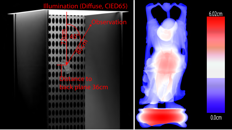
A virtual viewing booth with a dimension of depth x width x height = was designed employing a perfectly-diffuse area light emitter covering the whole ceiling of the booth. The spectral power distribution of the light is set to CIE D65 (daylight). The remaining parts of the booth have a gray value of CIE L and the back plane is covered with black circles, giving the observer additional hints for judging translucency, particularly in the optically thin range.
4.1.3. Sample and Viewing Geometry
Perceived translucency strongly depends on the shape -- particularly the thickness -- of an object. We used the Stanford Happy Buddha model11 1 https://graphics.stanford.edu/data/3Dscanrep/ with dimensions of depth x width x height . This model covers various surface orientations and thickness levels as shown in Figure 4. It also contains many thin regions that are particularly important for the human visual system to judge the degree of translucency (Fleming and Bülthoff, 2005; Nagai et al., 2013; Xiao et al., 2014). The model is placed into the booth so that its center has a distance of from the back plane and from the ceiling. The model’s length axis is rotated so that the model’s front side is illuminated from approx. 45∘. Renderings are computed from a viewpoint perpendicular to the model’s front side.
4.1.4. Sample selection
For the method of constant stimuli two pairs of samples are shown to subjects simultaneously: An anchor pair and a test pair. The anchor pair consists of two samples with a suprathreshold translucency difference (see Figure 5) and the scattering coefficients and . The test pair consists of a center sample and a test sample whose translucency difference is compared in a trial to the anchor pair (see section 4.2.2).
A first set of test pairs consists of samples with zero absorption: In a preliminary experiment, we selected 6 center samples at scattering coefficients . The perceived translucency difference between the center samples was selected to be clearly larger than the one of the anchor pair. For each center sample, we selected 7 test samples of increasing and 7 test samples of decreasing scattering coefficients. For the center sample with scattering coefficient only test samples of increasing and for center sample with scattering coefficient only test samples with decreasing scattering coefficients are used. We ensured that the maximum perceived difference between center sample and test sample in each direction is clearly larger than the one of the anchor pair and the minimum difference is clearly smaller. Each subject was shown a total of 6 (center samples) x 2 (directions) x 7 (test samples) - 2 (directions) x 7 (test samples) = 70 center/test pairs next to the anchor pair.
A second set of test pairs consists of samples with nonzero absorption. To make the results more robust to chromatic variations, we selected reference materials, but replaced the wavelength-independent absorption spectra by red, green and blue spectra, resulting in samples colored in the primaries of an RGB space. The anchor pair was always compared to a test pair possessing the same absorption spectrum and varying only in scattering, where scattering coefficients were selected in a similar way as for the first set of pairs. Note that the reflectance lightness values of these materials when measured according to Section 3 almost uniformly cover the range from to . For each of the three absorption spectra, a subject was shown 5 (center samples) x 2 (directions) x 6 (test samples) - 6 (directions) x 2 (test samples) = 58 center/test sample pairs next to the anchor pair, resulting in a total of 174 comparisons. See Appendix C for more details.
The position (left/right) of the anchor and test pairs was randomized during the experiment to minimize any sequential effects.
4.1.5. Viewing Conditions
The experiment was conducted in a dark room with no other source of illumination other than the display. Two color calibrated displays, the EIZO ColorEdge CG301W and CG276, were used in the experiments. The displays were calibrated to a white point of CIE D65. At the beginning of the experiment, the luminance of the rendering of a white opaque patch (perfectly reflecting diffuser) placed at the same position as the model was measured and a scaling factor was computed to set the patch’s luminance to . The luminance was directly measured on the displays with a Konica Minolta CS-1000A and a Topcon SR-3AR spectroradiometer. All renderings were than normalized using this scaling factor. For the method of constant stimuli, four wide renderings (anchor pair, center/test pair) are shown next to each other centered on the display. The remaining display area is set to the same gray color as the back panel of the virtual viewing booth. In the experiment, the subjects had a viewing distance of approx. from the display so that each image occupied approx. 4.8∘ and each model 4.24∘ of the visual field. For the original wide model, 4.24∘ of the visual field corresponds to a viewing distance of approx. .
4.2. Experiments
4.2.1. Subjects
A total of 40 subjects, 6 females and 34 males all with normal visual acuity according to the Snellen test participated in the experiment. All subjects passed the Ishihara color deficiency test. Their average age was 25.67 years with a standard deviation of 3.81 years.
4.2.2. Procedure
The anchor pair was shown with a center/test pair in random order on the display. The subjects were asked to select the pair that has the larger apparent translucency difference. No explicit definition of translucency was given to subjects but they were asked to not judge the difference of a pair based on color or overall lightness.

5. Psychometric Function and Modified Attenuation
5.1. Estimating visual translucency differences
For precise estimates of population tolerances, intra-observer uncertainty must be minimized. For this, we applied a low-pass filter algorithm on each observer’s binary data to reduce non-monotonic responses for each direction as suggested by Berns et al. (1991). We used Probit analysis on the resulting data to estimate the so called T50 distances from the selected sample centers. The T50 distance is the translucency difference from the sample center that is judged by 50% of the population to be smaller than the perceived translucency difference of the anchor pair and to be larger by the remaining 50% of the population.
Only T50 values for which the probit fit passed the goodness-of-fit test () were considered for the following evaluation. For the zero-absorption samples 8 out of 10, for the red and green 6 out of 8 and for the blue 4 out of 8 passed this test. A total of 24 visual translucency differences were considered. Rejections were characterized by a test sample choice spanning a too small visual translucency difference interval so that many observers found all test pairs in this direction to have a smaller translucency difference than the anchor pair.
For the second set of test pairs with red, green and blue absorption spectra, we computed for each material corresponding to a center sample and to the T50 distance the reference material as described in Section 3.3 using simulated measurements.
Figure 6 illustrates the Probit analysis for the transparent center sample. All data is provided in the supplementary material.
5.2. Simple models for the modified attenuation coefficient and the psychometric function
We aim to find simple models for and to obtain a perceptual uniformity for translucency comparable with the color uniformity of CIELAB. For this, we use a simple linear model for and Stevens’ power law for , yielding a two parameter model , if inserted into Eq. (1).
Since all visual translucency differences obtained in the visual experiment match with the anchor pair’s translucency difference, we can fit the model parameters by minimizing the disagreement of distances:
| (4) |
where is the set of the 24 different absorption and scattering pairs obtained in the visual experiment corresponding to a perceived translucency differences similar to the one of the anchor pair, is the distance in for the absorption and scattering pair , and corresponds to the anchor pair.
To evaluate the performance of the fit, we use the STandardized REsidual Sum of Squares (STRESS) index (see Appendix B). In our case the predicted difference is always and the visual translucency differences are . The STRESS index allows a significance comparison using the F-test.
The result of optimization (4) is with a STRESS value of 32,7. The numbers are already rounded to one decimal place without significantly changing the uniformity according to the F-test. Constant values employing this model are shown in Figure 3. For the not modified attenuation coefficient and without applying the psychometric function, i.e. , the STRESS value is 49.7. According to the F-test the uniformity for is significantly better than for . Figure 7 compares the performance of both models and Appendix D shows renderings of Lucy corresponding to a uniform sampling of both models for reference materials covering the visually-relevant absorption and scattering range. It is noteworthy that by non-linearly scaling the absorption parameter the STRESS value would further drop to 26.6. However, this would not significantly improve uniformity according to the F-test, it would require another parameter and it would break the modified attenuation coefficient’s unit. For this reason, we suggest to use the linear model for .
We also analyzed whether our model is overfitting the data using an exhaustive leave-one-out cross-validation test. The disagreements for the left-out visual translucency differences are: (mean, std, max) = (0.0352, 0.0255, 0.0857) and almost similar to the disagreements for all visual translucency differences (mean, std, max) = (0.0302, 0.0226, 0.0764). Also the model parameters are quite robust: (minp, meanp, maxp) = (0.31, 0,41, 0.47) and (minq, meanq, maxq) = (0.57, 0.58, 0.59), which suggest that the model does not overfit the data.
To put the STRESS index of 32.7 into perspective: The nearly-perceptually uniform CIELAB color space has a STRESS index of 43.93 on the COM data of experimentally determined color differences. The CIE94 color difference formula has a STRESS index of 32.1 and the best performing color difference formula (CIEDE2000) has a STRESS index of 27.49 on the COM data on which it was also optimized (Lissner and Urban, 2010).
6. Adjusting to the print size
In many situations, it is undesirable or even impossible to 3D print an object in its original size. Scaling the object up or down has implications for its perceived translucency, however. For example, if we consider a head or full-body scan of a human, given the build space capacities of state-of-the-art 3D printers, one would most likely print it smaller than the original size–a factor of 10 is common for retail full-body “mini-me" figurines. Using corresponding to the correct attenuation coefficients of human skin in this case would result in a print that looks far too translucent.
Fortunately, our definition of allows a simple adjustment so that resized models made of reference materials have perceptually similar translucency, as shown in Figure 8. For an object with homogeneous optical material properties, the amount of light exiting the surface of the object is governed by the extinction or attenuation coefficient . The mean free path, or average distance between scattering events is given by . The optical thickness or depth of an object is the number of mean free paths photons travel within it before being absorbed or exiting. By keeping fixed we keep the same. If we scale the object by a factor , the lengths of paths light travels will scale by , the number of scattering events will scale by , and will change accordingly. If we adjust so that, according to (1), the scattering and absorption coefficients ( are scaled by , we will get the same optical thickness as the original. The following formula accomplishes this
| (5) |
which is derived simply by plugging into (1).
Note that in Figure 8, the dot-texture in the background is kept at a fixed scale, so that the dots stay the same size, to clearly show the change in scale of the Buddha. This affects the appearance of the Buddha as the dot pattern becomes lower-frequency for the scaled-down rendering. The higher-frequency dot pattern in the larger-scale rendering is blurred by the light transport through the Buddha, resulting in a more uniform appearance–similarly to how a halftone pattern looks uniform to the human eye.

In Figure 9 we see a similar experiment, but the models printed using a recently proposed joint color and translucency pipeline (Brunton et al., 2018). In (b), we see a print with , while (a) shows a print with the same and (c) shows a print with scaled to match (b). Note that at the smaller size, surface roughness is more apparent in (c) compared to (b), altering the perception of translucency. However, considering the dramatic scale change, the adjusted matches the translucency of (b) quite well. Specific algorithmic choices of the pipeline may also have an influence, see Brunton et al. (2018) for details.

7. Approximating other materials
| height ( cm) | phase func. | () | () | A | Figure |
| Buddha | |||||
| iso. | 8 (left) | ||||
| iso. | 8 (middle) | ||||
| iso. | 8 (right) | ||||
| Dragon | |||||
| HG | Red∗ | 4 | 10a | ||
| iso. | 10b | ||||
| iso. | 10c∗∗ | ||||
| iso. | 10d | ||||
| iso. | 10e | ||||
| iso. | 10f∗∗ | ||||
| Lucy | |||||
| HG | Green∗ | 11a | |||
| iso. | 11b | ||||
| iso. | 11c | ||||
| HG | Green∗ | 11d | |||
| iso. | 11e∗∗ | ||||
| iso. | 11f∗∗ | ||||
| iso. | 11g | ||||
| iso. | 11h∗∗ | ||||
| Temple | |||||
| HG | Blue∗ | 12a | |||
| iso. | 12b | ||||
| iso. | 12c | ||||
| HG | Blue∗ | 12d | |||
| iso. | 12e∗∗ | ||||
| iso. | 12f∗∗ | ||||
| iso. | 12g | ||||
| iso. | 12h∗∗ | ||||
| ∗see Figure 15 in Appendix C for spectral absorption coefficients | |||||
| ∗∗post-process coloring (see Appendix G) | |||||


Our definition of represents a small fraction of possible optical materials, specifically a 2D subset spanned by the reference materials. We must therefore consider how to treat the remaining space of optical materials.
Given a material description in the form of optical material parameters, we can find the best matching reference material by simulating the measurement setup as described in Section 3 and linking the simulated measurements to the references materials as described in Section 3.3. In the top row of Figure 10, we see on the left the Stanford Dragon rendered with material properties not spanned by the reference materials, and in the middle we see the rendering with the reference material to which it is mapped. Figure 11 and 12 show the same for the Lucy and Temple model. Table 3 gives the parameter values for all renderings.
The measurement setup in Section 3 discards color information, as the reference materials are defined to have wavelength-independent absorption coefficients. An image-space post-process transfers color from the original to the reference rendering solely to simplify the comparison, as described in Appendix G. Note that the post-process does not change lightness contrast in the non-specular areas and thus preserves the translucency cues provided by the reference materials according to Motoyoshi (2010).
The selected materials should illustrate the limitations of our definition: They posses strong forward (Dragon) and backward (Lucy) scattering as well as a very dark (small lightness) material that is highly absorbing for almost all wavelength for which the luminous efficiency function of the HVS is high but almost transparent for other wavelengths (Temple) (see blue curve in Figure 15).
Using isotropic scattering to mimic forward scattering materials causes increasing lightness contrast for front/side-lit condition as can be seen in the Dragon’s leg area (compare Figure 10 (a) and (c)). The opposite can be seen for backward scattering where the lightness contrast is smaller for the reference materials as can be seen in Lucy’s chest region (compare Figure 11 (d) and (h)).
A very dark material with negligible scattering and wavelength-dependent absorption that is zero for a few wavelength shows higher apparent translucency than the best-fit reference material possessing a wavelength-independent high absorption causing incident light to be almost fully absorbed in the thick object (magnify Figures 12(a) and (b)/(c)). For the small Temple, light of all wavelengths is passing through the object causing luminance contrasts and thus the apparent translucency of original and reference material to be very similar (compare Figure 12 (d) and (c)/(h)).
7.1. of Real Materials
To validate as a translucency space for real materials, we conducted measurements of real materials, and printed patches using the resulting sRGB and values using the pipeline of Brunton et al. (2018). We chose samples of the following materials: a green wax, salmon, a green stone, a violet stone, and a green soap. Table 4 in Appendix E shows the measured sRGB and for a set of sample materials, and the results of putting those values through the 3D printing pipeline. Note that the errors reflect a combination of double measurement error (original and printed patch), plus gamut mapping and other reproduction errors (see Brunton et al. for details).
8. Limitations
Given we are consider just a one-parameter family of BSSRDFs, this comes with some limitations. By choosing an isotropic scattering function, is limited in its ability to approximate materials with anisotropic scattering. Figures 10, 11 and 12 show how well this approximation works for materials with different Heyney-Greenstein phase functions and spectral absorptions.
Measuring and assigning to heterogeneous materials works well if the heterogeneity is uniformly distributed, which importantly includes halftoned 3D printing materials used to characterized a printing system. However, stratified materials with a thickness exceeding the sample thickness used for measurements cannot be measured.
Our measurement setup is restricted to slab geometry, and measuring in the wild is a highly challenging problem, which we leave for future work.
Further, we propose as a translucency space, not a translucency appearance model, which has a number of consequences. The impact of other visual attributes, so called cross-contamination of visual attributes, is not considered, meaning the effect of gloss on perceived translucency is not modeled. The visual appearance of a material with a given is dependent on the defined viewing conditions (Sec. 4.1.5), and deviations from those conditions will affect the perceptual uniformity of .
9. Conclusion
We have presented a new interpretation, or redefinition, of the channel in RGBA, designed for graphical 3D printing, which replaces the traditional additive blending interpretation with a subtractive mixing one for material translucency. Our interpretation links to physical material measurements and embeds in a nearly perceptually uniform translucency scale for a set of virtual reference materials. By linking to these reference materials, we maintain device independence for both measurements and reproduction. Our definition allows simple adjustment to maintain consistent translucent appearance in the presence of object scaling, which is common in graphical 3D printing.
Our interpretation only considers isotropic phase functions, and therefore incorporating or adapting the interpretation to anisotropic phase functions of materials found in our environment is an important aspect of future work. Related to this is an investigation of the number of bits needed, from perceptual point of view, to sample , as defined in this paper, and how many bits are needed to either represent commonly used phase functions or to enumerate them. One option we consider promising is the notion of an -context, which would encompass additional parameters influencing the perception of translucency, such as phase function representations. Different contexts (phase functions) would give rise to different reference materials, and could themselves be standardized. We expect that printing materials for specific devices will mostly differ in terms of scattering and absorption, i.e. , rather than phase functions, which means contexts could be assigned to entire objects with spatially varying .
Other key direction for future work include further exploration of the link between perception of color and perception of translucency, and techniques to obtain for materials for which slab geometry is difficult to obtain.
Acknowledgements.
We thank the anonymous reviewers for their insightful and constructive comments. We thank Markus Barbieri for providing the design and Martin Majewski for creating the CAD data to simulate the Barbieri Spectro LFP, all observers who participated in our psychophysical experiment, and Can Ates Arikan for helpful discussions. This work was funded by the FhG Internal Programs under Grant No. Attract 008-600075, Scan4Reco project funded by EU Horizon 2020 Framework Programme under grant agreement no 665091 and AIF IGF-Vorhaben Nr. 18478 as well as JSPS KAKENHI Grant Number JP15H05922, JP16J00273 and the Leading Graduate School Program R03 of MEXT.References
- 3MF Consortium (2015a) 3MF Consortium. 2015a. 3MF file format specification. http://3mf.io/specification/. (2015).
- 3MF Consortium (2015b) 3MF Consortium. 2015b. 3MF Materials and Properties Extension. http://3mf.io/specification/. (2015).
- Arikan et al. (2015) C. A. Arikan, A. Brunton, T. M. Tanksale, and P. Urban. 2015. Color-Managed 3D-Printing with highly Translucent Printing Materials. In SPIE/IS&T Electronic Imaging Conference. San Francisco, 9398 – 9398 – 9.
- Attewell and Baddeley (2007) D. Attewell and R. J. Baddeley. 2007. The distribution of reflectances within the visual environment. Vision Research 47, 4 (2007), 548–554.
- Baar et al. (2014) T. Baar, S. Samadzadegan, H. Brettel, P. Urban, and M. V. Ortiz Segovia. 2014. Printing gloss effects in a 2.5 D system. In IS&T/SPIE Electronic Imaging. International Society for Optics and Photonics, 90180M–90180M.
- Barten (1999) P.G.J. Barten. 1999. Contrast sensitivity of the human eye and its effects on image quality. SPIE-International Society for Optical Engineering.
- Berns et al. (1991) R. S. Berns, D. H. Alman, L. Reniff, G. D. Snyder, and M. R. Balonon-Rosen. 1991. Visual determination of suprathreshold color-difference tolerances using probit analysis. Color Research and Application 16, 5 (1991), 297–316.
- Brunton et al. (2018) A. Brunton, C. A. Arikan, T. M. Tanksale, and P. Urban. 2018. 3D Printing Spatially Varying Color and Translucency. ACM Transactions on Graphics (TOG) 37, 4 (2018), 157:1–157:13.
- Brunton et al. (2015) A. Brunton, C. A. Arikan, and P. Urban. 2015. Pushing the Limits of 3D Color Printing: Error Diffusion with Translucent Materials. ACM Transactions on Graphics (TOG) 35, 1 (2015), 4.
- Chandrasekhar (1960) S. Chandrasekhar. 1960. Radiative transfer. Courier Dover Publications.
- CIE Publication No. 101 (1993) CIE Publication No. 101. 1993. Parametric Effects in Colour-difference Evaluation. Technical Report. Central Bureau of the CIE, Vienna, Austria.
- CIE Publication No. 159 (2004) CIE Publication No. 159. 2004. A colour appearance model for colour management systems: CIECAM02. CIE Central Bureau, Vienna.
- Cignoni et al. (2008) P. Cignoni, E. Gobbetti, R. Pintus, and R. Scopigno. 2008. Color enhancement for rapid prototyping. In VAST.
- Dong et al. (2010) Y. Dong, J. Wang, F. Pellacini, X. Tong, and B. Guo. 2010. Fabricating spatially-varying subsurface scattering. ACM Transactions on Graphics (TOG) 29, 4 (2010), 62:1–62:10.
- Elek et al. (2017) O. Elek, D. Sumin, R. Zhang, T. Weyrich, K. Myszkowski, B. Bickel, A. Wilkie, and J. Křivánek. 2017. Scattering-aware Texture Reproduction for 3D Printing. ACM TOG (Proc. of SIGGRAPH Asia) 36, 6 (2017), 241:1–241:15.
- Engeldrum (2000) P.G. Engeldrum. 2000. Psychometric Scaling: A Toolkit for Imaging Systems Development. Imcotek Press.
- Fairchild and Johnson (2004) M. D. Fairchild and G. M. Johnson. 2004. The iCAM framework for image appearance, image differences, and image quality. Journal of Electronic Imaging 13 (2004), 126–138.
- Faul (2017) R. Faul. 2017. Toward a Perceptually Uniform Parameter Space for Filter Transparency. ACM Transactions on Applied Perception (TAP) 14, 2 (2017), 13.
- Fleming and Bülthoff (2005) R. W. Fleming and H.H. Bülthoff. 2005. Low-level image cues in the perception of translucent materials. ACM Transactions on Applied Perception (TAP) 2, 3 (2005), 346–382.
- Gkioulekas et al. (2016) I. Gkioulekas, A. Levin, and T. Zickler. 2016. An Evaluation of Computational Imaging Techniques for Heterogeneous Inverse Scattering. In European Conference on Computer Vision. Springer, 685–701.
- Gkioulekas et al. (2013) I. Gkioulekas, B. Xiao, S. Zhao, E. H. Adelson, T. Zickler, and K. Bala. 2013. Understanding the role of phase function in translucent appearance. ACM Transactions on Graphics (TOG) 32, 5 (2013), 147.
- Goesele et al. (2004) M. Goesele, H. Lensch, J. Lang, C. Fuchs, and H.P. Seidel. 2004. DISCO: acquisition of translucent objects. ACM Transactions on Graphics (TOG) 23, 3 (2004), 835–844.
- Happel et al. (2014) K. Happel, E. Dörsam, and P. Urban. 2014. Measuring isotropic subsurface light transport. Optics express 22, 8 (2014), 9048–9062.
- Hašan et al. (2010) M. Hašan, M. Fuchs, W. Matusik, H. Pfister, and S. Rusinkiewicz. 2010. Physical reproduction of materials with specified subsurface scattering. ACM Transactions on Graphics (TOG) 29, 4 (2010), 61:1–61:9.
- ICC (2010) ICC. 2010. File Format for Color Profiles (4.3.0.0 ed.). http://www.color.org.
- ISO13655 (2009) ISO13655. 2009. Spectral measurement and colorimetric computation for graphic arts images. Technical Report. ISO 13655:2009 Graphic technology and photography.
- Jakob (2010) Wenzel Jakob. 2010. Mitsuba renderer. (2010). http://www.mitsuba-renderer.org.
- Jensen et al. (2001) H. W. Jensen, S. R. Marschner, M. Levoy, and P. Hanrahan. 2001. A practical model for subsurface light transport. In Proceedings of the 28th annual conference on Computer graphics and interactive techniques (ACM-SIGGRAPH). ACM, 511–518.
- Johnson and Fairchild (2003) G.M. Johnson and M.D. Fairchild. 2003. A top down description of S-CIELAB and CIEDE2000. Color Research and Application 28, 6 (2003), 425–435.
- Kubelka and Munk (1931) P. Kubelka and F. Munk. 1931. Ein Beitrag zur Optik der Farbanstriche. Zeitschrift für Technische Physik 12 (1931), 593–601.
- Lissner and Urban (2010) I. Lissner and P. Urban. 2010. Upgrading color-difference formulas. Journal of the Optical Society of America A 27, 7 (2010), 1620–1629.
- Lissner and Urban (2012) I. Lissner and P. Urban. 2012. Toward a Unified Color Space for Perception-Based Image Processing. Image Processing, IEEE Transactions on 21, 3 (2012), 1153–1168.
- MacAdam (1963) D. L. MacAdam. 1963. Nonlinear Relations of Psychometric Scale Values to Chromaticity Differencs. Journal of the Optical Society of America 53 (1963), 754–757.
- Melgosa et al. (2008) M. Melgosa, R. Huertas, and R. S. Berns. 2008. Performance of recent advanced color-difference formulas using the standardized residual sum of squares index. Journal of the Optical Society of America A 25, 7 (2008), 1828–1834.
- Montag and Berns (2000) E. D. Montag and R. S. Berns. 2000. Lightness dependencies and the effect of texture on suprathreshold lightness tolerances. Color Research & Application 25, 4 (2000), 241–249.
- Motoyoshi (2010) I. Motoyoshi. 2010. Highlight–shading relationship as a cue for the perception of translucent and transparent materials. Journal of vision 10, 9 (2010), 6–6.
- Nagai et al. (2013) T. Nagai, Y. Ono, Y. Tani, K. Koida, M. Kitazaki, and S. Nakauchi. 2013. Image regions contributing to perceptual translucency: A psychophysical reverse-correlation study. i-Perception 4, 6 (2013), 407–428.
- Naito et al. (2010) K. Naito, J. Yamada, T. Ogawa, and S. Takata. 2010. Measurement of scattering phase function of human skin. Japan Journal of Thermophysical Properties 24 (2010), 101–108.
- Peers et al. (2006) P. Peers, K. vom Berge, W. Matusik, R. Ramamoorthi, J. Lawrence, S. Rusinkiewicz, and P. Dutré. 2006. A compact factored representation of heterogeneous subsurface scattering. ACM Transactions on Graphics (TOG) 25, 3 (2006), 746–753.
- Porter and Duff (1984) T. Porter and T. Duff. 1984. Compositing digital images. SIGGRAPH Computer Graphics 18, 3 (1984), 253–259.
- Saunderson (1942) J. Saunderson. 1942. Calculation of the color of pigmented plastics. JOSA 32, 12 (1942), 727–729.
- Song et al. (2009) Y. Song, X. Tong, F. Pellacini, and P. Peers. 2009. SubEdit: A Representation for Editing Measured Heterogeneous Subsurface Scattering. ACM Transactions on Graphics (Proc. SIGGRAPH) (2009).
- Stevens (1960) S. S. Stevens. 1960. The psychophysics of sensory function. American scientist 48, 2 (1960), 226–253.
- Süsstrunk et al. (1999) S. Süsstrunk, R. Buckley, and S. Swen. 1999. Standard RGB color spaces. In IS&T/SID, 7th Color Imaging Conference. Scottsdale Ariz., 127–134.
- Ukishima et al. (2009) M. Ukishima, H. Kaneko, T. Nakaguchi, N. Tsumura, M. Hauta-Kasari, J. Parkkinen, and Y. Miyake. 2009. A Simple Method to Measure MTF of Paper and Its Application for Dot Gain Analysis. IEICE TRANSACTIONS on Fundamentals of Electronics, Communications and Computer Sciences 92, 12 (2009), 3328–3335.
- Urban et al. (2011) P. Urban, M. Fedutina, and I. Lissner. 2011. Analyzing small suprathreshold differences of LCD-generated colors. JOSA A 28, 7 (2011), 1500–1512.
- Watson and Ahumada (2011) Andrew B. Watson and Albert J. Ahumada. 2011. Blur clarified: A review and synthesis of blur discrimination. Journal of Vision 11, 5 (2011), 1–23.
- Wyble and Rich (2007) D. R. Wyble and D. C. Rich. 2007. Evaluation of methods for verifying the performance of color-measuring instruments. Part I: Repeatability. Color Research & Application 32, 3 (2007), 166–175.
- Wyszecki and Stiles (2000) G. Wyszecki and W.A. Stiles. 2000. Color Science: Concepts and Methods, Quantitative Data and Formulae (2 ed.). John Wiley & Sons, inc.
- Xiao et al. (2012) B. Xiao, I. Gkioulekas, A. Dunn, S. Zhao, E. Adelson, T. Zickler, and K. Bala. 2012. Effects of shape and color on the perception of translucency. In Vision Sciences Society Annual Meeting Abstract.
- Xiao et al. (2014) B. Xiao, B. Walter, I. Gkioulekas, T. Zickler, E. H. Adelson, and K. Bala. 2014. Looking against the light: How perception of translucency depends on lighting direction. Journal of vision 14, 3 (2014), 17–17.
- Yoshida et al. (2011) K. Yoshida, N. Komeda, N. Ojima, and K. Iwata. 2011. Simple and effective method for measuring translucency using edge loss: optimization of measurement conditions and applications for skin. Journal of biomedical optics 16, 11 (2011), 117003–1170038.
- Yule and Nielsen (1951) J. A. C. Yule and W. J. Nielsen. 1951. The penetration of light into paper and its effect on halftone reproduction. In Tech. Assn. Graphic Arts, Vol. 4. 65–76.
Appendix A Meaningful edge-loss measurements
In order to be meaningful, the edge-loss setup must measure lateral light transport effects visible for the human observer for a typical viewing distance. In other words: The low-pass filtering effect caused by lateral light transport detectable by the setup must be at spatial frequencies for which the human contrast sensitivity is not zero. To validate this, we used a set of isotropic point spread functions (PSF) , whose parameters are chosen so that for each integer resolution within the visible resolution range of [0, 50] cycles/degree (cpd) at least one PSF shows a decay of 50% assuming a viewing distance of 22 2 Gaussian-type PSFs were selected to create a range of blurring magnitudes without aiming to mimic PSFs of distinct materials.. For higher resolutions the achromatic contrast sensitivity is almost zero for office luminance conditions (Barten, 1999). We simulated the measurement of a material with a PSF parametrized by with an aperture for illumination as follows
| (6) |
where is the detection area, is the convolution operator and the irradiance is modeled by for and 0 elsewhere. This is a simplification because the irradiance within the illuminated area is generally not uniform for real spectrophotometers.
Figure 13 shows the edges-loss measurements for conditions and with . All edges-loss values are larger than and therefore detectable by spectrophotometers used in graphic arts.
Detection of these PSFs is one of two necessary criteria of the edge-loss measurement setup to be meaningful. The other is the ability to discriminate the blurring effect caused by these PSFs, which must be comparable or better than that of the HVS. The discrimination is limited by the repeatability error of the spectrophotometric measurments employing the two apertures. This repeatability error results in a measurement uncertainty that makes it impossible to discriminate PSFs with very similar edge-loss measurements; see particularly measurements for large cpd values in Figure 13. To discriminate two edge-loss measurements, we used a spectrophotometric discrimination threshold of based on average short-term repeatability errors of handheld spectrophotometer of and medium-term repeatability of (Wyble and Rich, 2007).
For estimating the ability of the HVS to discriminate two PSFs, we compared images blurred by these PSFs using the approach described by Johnson and Fairchild (Johnson and Fairchild, 2003). For a survey of other models of blur discrimination we refer to (Watson and Ahumada, 2011). As a test image containing a sharp edge with maximum contrast, we used the image described by , which models a disk-shaped uniformly illuminated area with a diameter of . For modeling light transport, we convoluted the image with the PSF (see Figure 14, right) and for modeling the contribution of the viewing distance, we convoluted the blurred image with the achromatic Contrast Sensitivity Function (CSF). We used the CSF employed by the iCAM framework for evaluating image differences (Fairchild and Johnson, 2004). Each of the 50 considered PSFs corresponds to an image blurred by light transport and the CSF. For comparing two PSFs, we computed pixel-wise lightness differences from the corresponding images and took the average employing only non-zero values. We assumed that for the blurring effects caused by the corresponding PSFs are not distinguishable by the HVS. Note that the perception of lightness and color differences depends on various factors, such as the luminance, sample size, texture, or background color (CIE Publication No. 101, 1993). For (the luminance of typical LCD displays), is below the just noticeable difference (JND) (Urban et al., 2011). Since the samples are non-uniform, the selected threshold is likely much lower than the real one (Montag and Berns, 2000), i.e. the ability of the HVS to discriminate lightness variations is even lower that assumed here.
Figure 14 compares the ability of the HVS and the spectrophotometric edge-loss setup to discriminate the evaluated PSFs. It shows that the instrument is either equally or more sensitive than the HVS. This statement holds even if we would increase the spectrophotometric discrimination threshold to . In summary, we can conclude that the edge-loss setup to measure lateral light transport employing common spectrophotometers used in graphic arts is meaningful with respect to typical viewing distances of approx. .

Appendix B Standardized residual sum of squares (STRESS) index
The STRESS index is used as a performance measure in multidimensional scaling (MDS) and to evaluate the performance of color difference equations (Melgosa et al., 2008). It is defined in our context as follows
| (7) | STRESS | ||||
where are computed and are visual translucency differences of a sample pair in a set of investigated pairs. The STRESS index is always in the range of [0,100], where 0 indicates a perfect agreement between computed and visual translucency differences. The larger the STRESS index the larger is the disagreement. The STRESS index allows a simple significance comparison between two formulas, and , computing translucency differences by comparing the term
| (8) |
with the critical value of the two-tailed -distribution with 95% confidence level and degrees of freedom: if , formula is significantly better than , if , formula is significantly poorer than , otherwise both formulas perform insignificantly different.
Appendix C Color Test Pairs

Appendix D Comparing Perceptual-Uniformity of and


Figure 17 demonstrates the perceptual uniformity of compared to that of . Figure 17a shows renderings of the Lucy model with scattering and absorption parameters corresponding to a uniform -sampling of the reference materials covering the visually-relevant absorption and scattering range, whereas Figure 17b shows the same for a uniform sampling in . The improvement of perceptual uniformity of compared to is particularly apparent in scattering ramps. Best view digitally by zooming in.
Since multiple reference materials correspond to the same - or -value, these renderings illustrate just one of many possible selections of reference materials. We selected for identical - or -values (diagonals in each subfigure) reference materials sampling the possible lightness reflectance range equidistantly.
Appendix E Measurments of Real Materials
Table 4 shows the sRGB and values measured for some real materials, and the errors of printed patches specified with those values using the pipeline of Brunton et al. (2018). The samples of violet stone, green stone and green soap can be seen in Figure 18 (right), and the results of printing with the values for green wax can be seen in Figure 20 (second from right).
| Material | Measured from original | Errors of printed patch | ||
|---|---|---|---|---|
| sRGB | A | CIEDE2000 | dA | |
| green wax | [0, 0.30, 0.27] | 0.6 | 3.4471 | 0.1323 |
| salmon | [0.89, 0.56, 0.33] | 0.72 | 6.1587 | 0.0413 |
| green stone | [0.39, 0.40, 0.20] | 0.49 | 2.8690 | 0.2509 |
| violet stone | [0.23, 0.05, 0.26] | 0.68 | 3.3113 | 0.0460 |
| green soap | [0.77, 0.82, 0.69] | 0.157 | 8.1293 | 0.0019 |
Appendix F Additional 3D Printed Examples
Here we show some 3D prints leveraging our definition. The prints are generated using a recently proposed joint color and translucency multimaterial 3D printing pipeline (Brunton et al., 2018). Figure 18 shows the St. Lucy model printed using the sRGB and values measured from 3 real samples (see Table 4), with linear transitions between them. Figure 19 shows a head model printed with an sRGB texture and two different values. Blurring of geometric and texture details increases for the lower . Figure 20 shows ships printed with the color values measured for wax (Table 4), and four different values, including that measured for wax. Different shape and magnitude of light transport are visible for different values.


Appendix G Color Adjustment of Reference Material Renderings
To make translucency comparisons easier for materials with spectrally non-uniform absorption, we transfer color in image space from the rendering of the original material to the resulting reference material with the following post-process, which does not change the lightness contrast in the non-specular areas and preserves the translucency cues provided by the reference materials according to Motoyoshi (2010). Given an input material, its measurements according to the setup in Section 3 along with the resulting reference material, and a rendering of an object with the original material:
- •
We render the same object with the same illumination and viewing conditions as the original with the reference material.
- •
Since specular highlights are dominated by Fresnel reflection, which is similar for both the original and reference materials, but also influenced by absorption, we copy and paste specular highlights from the original rendering into the output rendering using a mask.
- •
Since is not a measure of lightness (which is included in the scale-invariant RGB) we adjust the median lightness of the reference rendering to match the median lightness of the original rendering for non-specular pixels. The median lightness is used to mitigate potential influence of remaining specularities.
- •
Finally, for non-specular pixels, we copy the CIELAB a* and b* values from the original rendering to the reference rendering so that they have the same hue.
We applied this process to Figures 10(c, f), 11(e, f, h) and 12(e, f, h), to make them easier to compare to Figures 10(a), 11(a) and 12(a).