Signatures of van der Waals binding: A coupling-constant scaling analysis

Coupling-constant scaling analysis[8] is a natural tool for exploring the nature of both exchange-based GGAs[11, 57] and of vdW-DF-cx. For any given solution density $n(\mathbf{r})$, we define a rescaled density

and resolve Eq. (14) into $\lambda$-specific contributions using the exact result[8, 11, 57]

Since there is no $\lambda$ dependence for exchange, we can recast Eq. (22) using the correlation-energy density:

The scaling results for $E_{{\rm xc},\lambda}[n]$ and $e_{{\rm c},\lambda}[n]$ can be directly applied to individual components of the XC functional (as they are linear in the functional expression).

The scaling results, Eqs. (22) and (23), reflect properties of the $\chi_{\lambda}$ approximations that are implicitly made in crafting the PBE and vdW-DF-cx functionals. The existence of a well-understood coupling-constant scaling has been used to rationalize the formulation of the PBE0 hybrid[70] based on PBE.[11, 57] Noting that a similar rationale exists for the coupling constant scaling of vdW-DF-cx, some of us have recently motivated the introduction of correspondingly defined vdW-DF hybrids, including vdW-DF-cx0, which replace the vdW-DF-cx exchange component with a fraction of Fock exchange.[71]

The scaling results, Eqs. (22) and (23), follow from an analysis of the many-particle wavefunction ground-state solution $\Psi_{n}^{{\rm min},\lambda}$ corresponding to a specific density $n$ and a specific strength $\lambda V$ of the electron-electron interaction. The detailed arguments are given elsewhere; For completeness, we include a renormalization-type argument for this observation in the appendix. Here we simply note that the wavefunctions solving the Hamiltonian $\hat{H}=\hat{T}+\lambda V+V_{\rm ext}$ themselves scale according to

and that this formal equivalence is sufficient to establish the $\lambda$ scaling.[8, 11]

Below we drop explicit references to the density functional nature when working with spatially-resolved energy contributions such as $e_{{\rm c},\lambda}^{\rm nl}(\mathbf{r})$ and $e_{{\rm c}}^{\rm nl}(\mathbf{r})$, except when specifically needed for the discussion.

In the KS scheme [7], we nominally focus on computing the so-called KS kinetic energy²² 2 In discussions of DFT, $T_{\rm KS}$ is sometimes called the single-particle kinetic energy. We prefer the Kohn-Sham label as $\hat{T}$ is always a single-particle operator. from single-particle expectation values

for occupied orbitals $\phi_{i}(\mathbf{r})$. As in the Quantum-Espresso package,[73] we compute the KS kinetic energy as a spatial integration

over positive definite contributions

defined by the set of occupied orbitals. This representation of the KS kinetic energy is simply related to the summation $\tilde{t}_{\rm occ}(\mathbf{r})\equiv\Sigma_{i}^{\rm occ}\tilde{t}_{i}(\mathbf{r})$ over single-particle contributions, Eq. (26). The descriptions differ only in the inclusion of an Poisson-type term

and give the same total KS kinetic energy, Eq. (27), upon spatial integration.

We typically compute DFT energies $E^{\rm A/B/AB}_{\rm DFT}$ of combined systems ‘AB’ and of the relevant fragments, ‘A’ or ‘B’, to understand binding $\Delta E_{\rm DFT}=E^{\rm A}_{\rm DFT}+E^{\rm B}_{\rm DFT}-E^{\rm AB}_{\rm DFT}$ (with suitable adjustments in the case of related problems such as material cohesion). The mean-field electrostatic energy among electrons, that is, the Hartree term

is one important contribution as it approximates $\langle\hat{V}\rangle$. For analysis, we track binding-induced changes like

We also track corresponding expressions for binding-induced changes in, for example, the total nonlocal-correlation term $\Delta E_{\rm c}^{\rm nl}$. In our discussion, we call such differences binding contributions.³³ 3 The wording ‘binding contribution’ is used to describe any component of the molecular binding even if, for example, $\Delta T_{\rm c}(\mathbf{r})$ is negative. Similarly, we use the word ‘spatially resolved binding contributions’ to describe binding-induced changes in the spatial variation of, for example, XC energy terms, like $\Delta e_{\rm c}^{\rm nl}(\mathbf{r})$; Again this term is used without regards to the sign of the integrated values.

Computational results for the binding-induced changes in the KS kinetic energy $\Delta T_{\rm KS}$ and in the mean-field electrostatic energy $\Delta U[n]$ often suffice for a characterization of covalent bonds in molecules and materials.[75] This is because the combination allows us to characterize and understand orbital hybridization.[75, 76, 77] However, for noncovalent bonds we have to look further than changes in $T_{\rm KS}$. One can generally sort chemical bonds from knowledge of the average orbital energy.[78] The average orbital energy is a measure that will, in principle, reflect all correlation effects, including those that are manifested in the kinetic energy.

A formal analysis of the DFT variational scheme[8] shows that

where $\alpha\equiv 1/\lambda$, Refs. 8, 11. Using the density-scaling analysis, it immediately follows that

A similar equation connects $T_{\rm c}^{\rm nl}[n]$ and $E_{\rm c}^{\rm nl}[n]$. For any given system (solution density $n$), we use numerical differentiation to compute $E_{{\rm c},\lambda}[n]$ and $E_{{\rm c},\lambda}^{\rm nl}[n]$ from Eq. (22), and $T_{\rm c}[n]$ and $T_{\rm c}^{\rm nl}[n]$ from Eq. (34).

The electron-electron interaction effects in the physical systems are now formally available for computation (in the approximations that define $E_{\rm xc}[n]$). In particular, we can study the electrodynamical coupling among plasmons[1, 4, 3, 6] at $\lambda=1$ since $E_{{\rm c},\lambda=1}^{\rm nl}[n]$ is available via Eq. (35). This value $E_{{\rm c},\lambda=1}^{\rm nl}[n]$ is the nonlocal-correlation part of $E_{{\rm xc},\lambda=1}[n]$ which, by definition, is given by a contour integral of the response $\chi_{\lambda=1}$ evaluated at full electron-electron interaction strength, Eqs. (11) and (13).

We note in passing that $E_{{\rm c},\lambda=1}^{\rm nl}[n]$ is also the nonlocal-correlation part of the electron-electron interaction expectation value

Since the XC energy functional is defined $E_{\rm xc}=\langle\hat{V}+\hat{T}\rangle-T_{\rm KS}-U[n]$ we can use Eq. (35) for the formal identification

The formal equivalence Eq. (36) follows by subtracting the LDA and gradient-corrected exchange components.

Figure 1 shows (computed results for) the coupling constant scaling for the XC contribution (solid red curve) to the total energy of the N₂ molecules. The specific scaling results are here provided for vdW-DF-cx (using the formal derivation of the scaling for $E_{\rm c}^{\rm nl}$ detailed in the following subsection): However, the behavior is generic and thus similar to what has previously been reported and discussed for PBE.[11, 57]

We note that the exchange and correlation components, $E_{\rm x}$ and $E_{\rm c}$, used for DFT calculations in the KS scheme, are integrals of the indicated $\lambda$ variations. The exchange value traces a horizontal line (dotted curve separating red and green areas) in Fig. 1. In contrast, the correlation begins at zero but changes to a significant magnitude at $\lambda=1$. It is straightforward to verify[11] that the area of the green region is minus the functional approximation for $E_{\rm c}$. Importantly, we can immediately extract the corresponding kinetic-correlation energy $T_{\rm c}$ using Eq. (35), that is, as the area of the blue region below the $E_{{\rm xc},\lambda}$ variation but above the value of the $\lambda\to 1$ limit.

To compute the kinetic-energy component of vdW binding, we need only consider the density scaling for the correlation parts, namely $E_{c}=E_{c}^{\rm LDA}+E_{c}^{\rm nl}$. Moreover, the coupling constant scaling for the LDA part, $E_{c}^{\rm LDA}$, has previously been discussed, as it is part of the GGA characterization.[8, 79, 9, 10, 55, 80, 56, 57, 11]

To explore the coupling-constant scaling of $E_{\rm c}^{\rm nl}$ we first summarize the vdW-DF formulation of this nonlocal-correlation energy. Any semilocal XC density functional can be characterized by a local energy-per-particle density

where $\epsilon_{\rm xc}[n](\mathbf{r})$ is a function of just the local density $n(\mathbf{r})$ and the scaled density gradient $s(\mathbf{r})$. We further split $\epsilon_{\rm xc}[n](\mathbf{r})$ into exchange and correlation components, $\epsilon_{\rm x}[n](\mathbf{r})$ and $\epsilon_{\rm c}[n](\mathbf{r})$. The local variation in the inverse length scale $q_{0}$ for the plasmon-pole description can then be expressed [15, 16]

Here $k_{F}=(3\pi^{2}n)^{1/3}$ denotes the local value of the Fermi wave-vector and $\varepsilon_{x}^{\rm LDA}=-3k_{F}/4\pi$ is the energy-per-particle density in LDA exchange. The nonlocal-correlation energy is computed[15]

using a universal-kernel formulation,[15, 33, 16, 27]

The universal kernel $\Phi_{0}(d,d^{\prime})$ is tabulated and permits an efficient numerical evaluation through fast-Fourier transforms.[27] The generalization to scaling in spin-polarized cases is also completely specified, since it amounts to a simple rescaling of the inverse length scale $q_{0}$, Ref. 19.

For scaling analysis (and coding), it is convenient to introduce $\tilde{\mathbf{r}}\equiv\mathbf{r}/\lambda$ as a short hand for the coordinate scaling and to represent the density variation in terms of $r_{s}(\mathbf{r})=(3/4\pi n(\mathbf{r}))^{1/3}$. The local values of the scaled density gradient are $s(\mathbf{r})=|\nabla n|/(2k_{F}(\mathbf{r})n(\mathbf{r}))$. The density scaling $n(\mathbf{r})\to n_{1/\lambda}(\mathbf{r})=n(\tilde{\mathbf{r}})/\lambda^{3}$ leaves $s$ unchanged and the effect amounts to computing the changes in Fermi vector and in the LDA correlation components. This is done in terms of the corresponding scaling $r_{s}(\mathbf{r})\to\lambda r_{s}(\tilde{\mathbf{r}})$.

Using $F_{x}(s)$ to denote the exchange-enhancement factor of $E_{\rm xc}^{\rm in}$, the overall scaling of the inverse length scale can be expressed $q_{0}[n_{1/\lambda}(\mathbf{r})]=q_{0}^{\lambda}(\tilde{\mathbf{r}})$, where

Introducing also

we can compute

We complete the scaling analysis of $E_{\rm c}^{\rm nl}$ via Eq. (22) and of $e_{\rm c}^{\rm nl}(\mathbf{r})$ via Eq. (23). Specifically, we express the scaling of the nonlocal-correlation energy density

For the numerical evaluation we adopted the scheme proposed by Román-Pérez and Soler [27] (as implemented in quantum-espresso) to calculate $e_{\rm c}^{\rm nl}[\lambda r_{s}(\mathbf{\tilde{r}})]$; the calculation is similar to the calculation of $e_{\rm c}^{\rm nl}(\mathbf{r})$ in Ref. 31. We note that $e_{{\rm c},\lambda=1}(\mathbf{r})$ provides a spatial mapping of all nonlocal-correlation effects that exist in the fully interacting system, as a direct implication of Eq. (35).

Moreover, as part of this $e_{{\rm c},\lambda=1}(\mathbf{r})$ characterization, we can now compute the spatially resolved kinetic-correlation energy $t_{\rm c}(\mathbf{r})$ and nonlocal-kinetic-correlation energy $t_{\rm c}^{\rm nl}(\mathbf{r})$. First, we simply add the known[8, 9, 10, 55] coupling constant scaling of the LDA correlation-energy density, $e_{{\rm c},\lambda}^{\rm LDA}$, entering in Eq. (18):

Next, we adapt Eq. (34) to descriptions of energy densities

and evaluate the derivatives numerically.

Figure 2 documents the coupling-constant scaling of $E_{{\rm c},\lambda}^{\rm nl}$ and explains an approximately linear variation. The top panel shows the coupling-constant scaling for the ratio $q_{0c}/q_{0x}$ for typical contributions to the binding of an N₂ molecule. Specifically, starting from the known $q_{0x}(n(\mathbf{r}))$ and $q_{0c}(n(\mathbf{r}))$ values, the panel traces the variation in the XC components of $q_{0}(n_{1/\lambda}(\mathbf{r}))$ for conditions that roughly correspond to the binding region of N₂ (red curves) and to electron density tails of atoms and molecules (blue curves).

The middle panel of Fig. 2 shows the coupling-constant scaling of $E_{\rm c}^{\rm nl}[n_{1/\lambda}]$ (solid curve) for the density of the N₂ molecule. We note that the scaling in $q_{0x}$ is exactly offset by the $\lambda$ scaling of coordinates in Eqs. (46) and (47). Thus if we assume that the scaling of $q_{0}=q_{0x}+q_{0c}$ is set by the scaling in $q_{0x}$, there would be no $\lambda$-dependence in the $E_{\rm c}^{\rm nl}$ kernel arguments, $d=q_{0}(\mathbf{r})|\mathbf{r}-\mathbf{r^{\prime}}|$ and $d^{\prime}=q_{0}(\mathbf{r^{\prime}})|\mathbf{r}-\mathbf{r^{\prime}}|$. In this type of approximations there is then no scaling in the corresponding approximations for $E_{\rm c}^{\rm nl}[n_{1/\lambda}]$.

The middle panel furthermore shows two potentially relevant such approximations motivated by the analysis of the typical variations in the $q_{0c}/q_{0x}$ ratio. The first assumes that we can ignore the influence of the correlation part $q_{0c}$ completely (giving the green dashed-dotted line); the second assumes that the ratio $q_{0c}/q_{0x}$ can at any given point $\mathbf{r}$ be taken as fixed at the $\lambda=1$ value (giving the blue dashed curve). The second choice effectively amounts to simply setting $E_{\rm c}^{\rm nl,linear}[n_{1/\lambda}]\equiv E_{\rm c}^{\rm nl}[n]$. Neither of them is a good description for Eq. (48). On the other hand, we add a $\lambda^{2}$ weight on $E_{\rm c}^{\rm nl}[n_{1/\lambda}]$ when computing $E_{{\rm xc},\lambda}$, Eq. (22). We label the second approximation as ‘linear’ since it leads to $E_{{\rm c},\lambda}^{\rm nl}\approx\lambda E_{\rm c}^{\rm nl}[n]$ and this is sometimes an acceptable approximation.

The bottom panel of Fig. 2 contrasts the resulting scaling of the ACF integrand for the nonlocal correlation contribution $E_{{\rm c},\lambda}^{\rm nl}[n]$ against that of the LDA correlation $E_{\rm c}^{\rm LDA}[n]$. The panel also shows (green and blue dashed curves) the scaling that results by inserting either of the approximations discussed in the middle panel into Eq. (22). Interestingly, the scaling relevant for the N₂-molecule total energy is found well approximated by using $E_{\rm c}^{\rm nl,linear}[n_{1/\lambda}]\equiv E_{\rm c}^{\rm nl}[n]$. The nonlocal-correlation part of the kinetic energy is just minus the total nonlocal-correlation binding contribution $\Delta E_{\rm c}^{\rm nl}$ in such special cases.

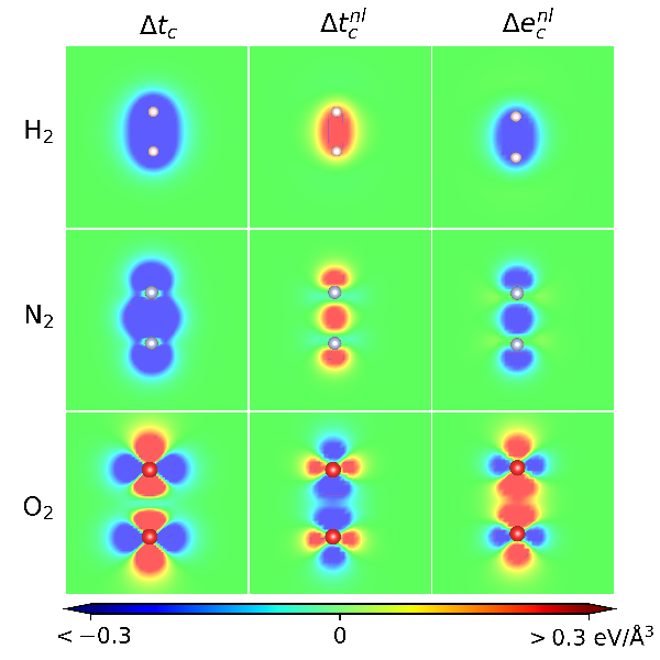
Figure 4 shows that the kinetic-correlation energy is important in characterizations of intra-molecular binding. The figure details the spatial variation in the kinetic-correlation binding energy contribution $\Delta t_{\rm c}$, in the nonlocal-correlation-kinetic energy contribution $\Delta t_{\rm c}^{\rm nl}$, and in the vdW-DF-cx nonlocal correlation energy binding contribution $\Delta e_{\rm c}^{\rm nl}$ for the H₂, N₂, and O₂ molecules.

We note that the magnitude of the variation in $\Delta t_{\rm c}$ is about an order-of-magnitude smaller than the KS kinetic-energy binding contribution $\Delta t_{\rm KS}(\mathbf{r})$ (not shown) for these covalently bonded systems. Nevertheless, there is clear structure in both $\Delta t_{\rm c}^{\rm nl}(\mathbf{r})$ and $\Delta e_{\rm c}^{\rm nl}(\mathbf{r})$ and a directed nature or signature of vdW interactions even in these strongly bonded dimer molecules.

Supplementary materials Tables S.I and S.II, supported by Fig. S1, provides a broader analysis of such intra-molecular bindings. This is done both for the set of molecules for which there already exists a PBE-based coupling-constant analysis,[11, 57] and for the G2-1 benchmark set of molecular atomization energies. Most of these systems are covalently bonded, meaning that orbital hybridization plays the decisive role. However, there are also some G2-1 cases, for example, alkali dimers, where the nonlocal-correlation energy and the nonlocal part of kinetic-correlation energy are important. Here, in the main text we concentrate on characterizing the binding in H₂, N₂, and O₂.

The O₂ kinetic-correlation energy binding contribution $\Delta t_{\rm c}$ deserves a special discussion. The first O₂ panel of Fig. 4 shows the variation of $\Delta t_{\rm c}(\mathbf{r})$ in a plane that contains the binding axis in the dimer. This plot has areas of opposite signs and implies a compensation. However, the overall kinetic-correlation energy contribution is still negative, $\Delta T_{\rm c}<0$, because the negative regions, away from the axis, have greater weight as we perform the spatial integration. The total, negative kinetic-correlation energy binding contribution is given by the light blue area shown in the left column in Fig. 3.

The second column of Fig. 4 shows the spatial variation in the nonlocal-correlation part of the kinetic-energy binding contribution, $\Delta t_{\rm c}^{\rm nl}(\mathbf{r})$, for the three molecules. The variation in $\Delta t_{\rm c}(\mathbf{r})$ (first column) is generally dominated by the LDA contribution but adjusted by the variation in $\Delta t_{\rm c}^{\rm nl}(\mathbf{r})$. The integrated binding contribution from the nonlocal part of the kinetic-correlation energy $\Delta T_{\rm c}^{\rm nl}$ can be both negative or positive (as exemplified by the H₂ and N₂ cases). In such positive-$\Delta T_{\rm c}^{\rm nl}$ cases, the binding contribution from $E_{\rm c}^{\rm nl}$ is negative, i.e., the nonlocal-correlation energy is actually causing a repulsion in these intra-molecular binding cases. The supplementary materials Tables S.I and S.II provide a broader overview of the variation in nonlocal-correlation energy and kinetic-correlation energy effects that we document for intra-molecular binding.

The third column of Fig. 4 shows a mapping of the nonlocal-correlation energy contribution to binding, $\Delta e_{\rm c}^{\rm nl}(\mathbf{r})$, allowing a contrast with the variation documented for $\Delta t_{\rm c}(\mathbf{r})$ and $\Delta t_{\rm c}^{\rm nl}(\mathbf{r})$. We find that $\Delta e_{\rm c}^{\rm nl}(\mathbf{r})$ and $\Delta t_{\rm c}^{\rm nl}(\mathbf{r})$ are here essentially negative prints of each others. It follows that the full ($\lambda=1$) nonlocal-correlation energy contribution, given by $\Delta e_{\rm c}^{\rm nl}(\mathbf{r})-\Delta t_{\rm c}^{\rm nl}(\mathbf{r})$ remains qualitatively described by the variation in $\Delta e_{\rm c}^{\rm nl}(\mathbf{r})$ in these cases.

Supplementary materials Tables S.I and S.II show that the nonlocal-correlation energy binding contribution $\Delta E_{\rm c}^{\rm nl}$ can take either sign for intra-molecular binding. These tables also show that $\Delta T_{\rm c}^{\rm nl}$ will typically then have the opposite sign. We therefore generally expect the $\Delta e_{\rm c}^{\rm nl}(\mathbf{r})$ and $-\Delta t_{\rm c}^{\rm nl}(\mathbf{r})$ contributions to mirror each other, as in Fig. 4. The implication is that $\Delta e_{\rm c}^{\rm nl}(\mathbf{r})$ provides a qualitatively correct mapping of the vdW interaction in most covalently bonded cases.

Finally, we note that there are exceptions to this general trend, i.e, cases where $\Delta T_{\rm c}^{\rm nl}$ and $\Delta E_{\rm c}^{\rm nl}$ are both negative. Figures S1 and S2 in the supplementary materials, provide additional analysis for one of these cases, namely P₂. In such cases it is in principle necessary to compute both the $\Delta e_{\rm c}^{\rm nl}(\mathbf{r})$ and the $\Delta t_{\rm c}^{\rm nl}(\mathbf{r})$ variation to obtain a complete mapping, $\Delta e_{\rm c}^{\rm nl}(\mathbf{r})-\Delta t_{\rm c}^{\rm nl}(\mathbf{r})$, Fig. S2. However, even in these cases it is still so that $\Delta e_{\rm c}^{\rm nl}(\mathbf{r})$ and the $-\Delta t_{\rm c}^{\rm nl}(\mathbf{r})$ are approximately mirrors of each others. That is, even in P₂, there is no change in the qualitative observations presented above.

Figure 5 compares kinetic-energy binding contributions $\Delta t_{\rm tot}(\mathbf{r})$, $\Delta t_{\rm KS}(\mathbf{r})$, $\Delta t_{\rm c}(\mathbf{r})$, $\Delta t_{\rm c}^{\rm nl}(\mathbf{r})$, in non-covalently bonded systems, i.e., in cases where there is no pronounced orbital hybridization. The top row shows our vdW-DF-cx based results for a benzene dimer, a case which is expected to have an essentially pure vdW (or dispersion) interaction. The bottom row shows results for a water dimer, a case that is predominantly hydrogen bonded, while the middle row explores the mixed-binding benzene-water case.

The supplementary materials Table S.III, supported by Fig. S3, provides a broader characterization of binding in the S22 benchmark set of such weakly bonded molecular complexes. In all of theses cases, the nonlocal-correlation energy contribution $\Delta E_{\rm c}^{\rm nl}$ is positive while $\Delta T_{\rm c}^{\rm nl}$ is negative. As such, the following discussion is generic.

For reference, the last column of Fig. 5 shows the spatial variation in the nonlocal-correlation energy binding, $\Delta e_{\rm c}^{\rm nl}(\mathbf{r})$. This binding plays a decisive role in all cases. It is a core component of our vdW-DF-cx characterization and it is important for an accurate description of these molecular complexes.[18] In the case of dispersion-bonded systems, the $\Delta e_{\rm c}^{\rm nl}(\mathbf{r})$ contributions are the only sources of cohesion; In the case of the water dimer and the benzene-water complexes, there are also significant electrostatic components in the inter-molecular interactions.

The first, second, and third columns of Fig. 5 contrast the spatial variation in the binding contributions from the total kinetic energy, from the KS kinetic energy, and from the kinetic-correlation energy. There are no orbital hybridization effects in play, but it is important to note that the $E_{\rm c}^{\rm nl}$ binding also pushes densities and thus orbitals around. Smaller signatures are therefore retained in the binding contribution from the KS kinetic energy, $\Delta t_{\rm KS}(\mathbf{r})$.

Contrasting the panels in the first and second column of Fig. 5, we find that the KS kinetic-energy effects are still the major source of the variation that we compute for $\Delta t_{\rm tot}(\mathbf{r})$. Nevertheless, in the case of dispersion-bonded systems, we find that there are also important contributions from the kinetic-correlation energy $\Delta t_{\rm c}(\mathbf{r})$. These contributions, shown in isolation in the third column, arise primarily in the inter-molecular region, in areas that have a sparse[34] (but not vanishing) electron density and small-to-moderate density gradient. We sometimes refer to these binding parts as a trough[18, 6] but we are then emphasizing the presence of important internal surfaces within such sparse intermolecular regions.[14, 35, 34]

The enhanced binding contributions from internal surfaces reflect the many-electron nature of the vdW problem. The amplitudes of collective (plasmon) excitations are themselves enhanced in the sparse surface-like intermolecular region and we should then expect larger contributions to the systematic tracking of the electrodynamical coupling among plasmons.[1, 2, 4, 3, 5, 14, 15, 6, 20] The vdW enhancement can also be interpreted as reflecting image-plane effects at (internal or external) surfaces,[39, 40, 41, 14, 110, 63, 111, 112] or as multipole response-effects effects when arising outside molecules.[25, 26, 35, 36, 113, 114, 115] In any case, the vdW-DF-cx handling of screening[1, 3, 15, 24, 6] provides mechanisms to track the expected vdW enhancement in the sparse intermolecular regions, at important internal surfaces.[14, 32, 37, 6]

The fourth column of Fig. 5 shows the nonlocal part of the kinetic-correlation energy, $\Delta t_{\rm c}^{\rm nl}(\mathbf{r})$. Contrasting the third and fourth columns makes it clear that the LDA component of $\Delta t_{\rm c}(\mathbf{r})$ generally masks the variation in $\Delta t_{\rm c}^{\rm nl}(\mathbf{r})$. However, the signatures of the nonlocal kinetic-correlation part dominate in the spare-density regions for dispersion-bonded systems. The nonlocal part also remains a non-vanishing part of full kinetic-correlation energy in the hydrogen-bonded and mixed binding cases.

Figure 6 shows the computed binding contributions in the stacked uracil dimer and in the stacking of adenine and thymine. The top row shows the investigated geometries from the S22 benchmark set.[109] Supplementary materials Fig. S.4 shows the variation in the kinetic-energy binding contributions for these systems.

The panels in the bottom two rows of Figure 6 contrast the variation in the $\Delta e_{\rm c}^{\rm nl}$ and $\Delta e_{{\rm c},\lambda=1}^{\rm nl}=\Delta e_{\rm c}^{\rm nl}(\mathbf{r})-\Delta t_{\rm c}^{\rm nl}(\mathbf{r})$ accounts of the nonlocal-correlation binding. The contributions are computed for the cuts indicated by the two dashed lines in the top panels. We find that including the nonlocal part of the kinetic-correlation energy enhances the binding signatures found in the $\Delta e_{\rm c}^{\rm nl}$ variation in our mapping of the total nonlocal correlation binding, shown in the pair of lower panels. The same is true for the wider set of S22 cases. Comparing the fourth and fifth column of Fig. 5 we see that they are essentially negative prints of each other, i.e., naturally leading to an enhancement of signatures in $\Delta e_{\rm c}^{\rm nl}(\mathbf{r})-\Delta t_{\rm c}^{\rm nl}(\mathbf{r})$.

For both inter- and intra-molecular interactions the variation, $\Delta e_{{\rm c},\lambda=1}^{\rm nl}(\mathbf{r})$ can effectively be mapped using either $\Delta e_{\rm c}^{\rm nl}(\mathbf{r})$ or $-\Delta t_{\rm c}^{\rm nl}(\mathbf{r})$.

We also find that the $\Delta e_{{\rm c},\lambda=1}^{{\rm nl}}(\mathbf{r})$ signatures are, in effect, channelled into pockets of binding, Figs. 5 and 6. The dominant contributions are located in the intermolecular (trough) regions but concentrated in areas that resemble orbitals. In other words, we can, in principle, use a similar form of bond-type characterization for a qualitative discussion of the nonlocal-correlation binding, drawing on an analogy with discussions of chemical bonds.

Before using this vdW-bond mapping analysis, below, we emphasize that this binding is much weaker and that the concentration of binding (in such inter-molecular pathways) arises for a different physical reason[16] than in chemical bonds. Chemical binding can exist in the $\lambda\to 0$ limit (in a Hartree-Fock description) by orbital hybridization, but that cannot happen for the nonlocal-correlation (or vdW) binding. While the inclusion of the $E_{\rm c}^{\rm nl}$ energy term in DFT calculations causes density changes, and therefore an electrostatic signature,[16] the total nonlocal-correlation binding reflects, instead, an energy gain[16] produced by collective exitations, i.e., by plasmons described by the screening properties.[1, 4, 12, 14, 15, 116, 6]

References

- [1] G. D. Mahan, J. Chem. Phys. 43, 1569 (1965).
- [2] D. C. Langreth and J. P. Perdew, Phys. Rev. B 15, 2884 (1977).
- [3] K. Rapcewicz and N. W. Ashcroft, Phys. Rev. B 44, 4032 (1991).
- [4] A. C. Maggs and N. W. Ashcroft, Phys. Rev. Lett. 59, 113 (1987).
- [5] D. C. Langreth and S. H. Vosko, Phys. Rev. Lett. 59, 497 (1987).
- [6] P. Hyldgaard, K. Berland, and E. Schröder, Phys. Rev. B 90, 075148 (2014).
- [7] W. Kohn and L. J. Sham, Phys. Rev. 140, A1133 (1965).
- [8] M. Levy and J. P. Perdew, Phys. Rev. A 32, 2010 (1985).
- [9] M. Levy, Phys. Rev. A 43, 4637 (1991).
- [10] A. Görling and M. Levy, Phys. Rev. B 47, 13105 (1993).
- [11] K. Burke, M. Ernzerhof, and J. P. Perdew, Chem. Phys. Lett. 265, 115 (1997).
- [12] Y. Andersson, D. C. Langreth, and B. I. Lundqvist, Phys. Rev. Lett. 76, 102 (1996).
- [13] H. Rydberg, B. I. Lundqvist, D. C. Langreth, and M. Dion, Phys. Rev. B 62, 6997 (2000).
- [14] H. Rydberg, M. Dion, N. Jacobson, E. Schröder, P. Hyldgaard, S. I. Simak, D. C. Langreth, and B. I. Lundqvist, Phys. Rev. Lett. 91, 126402 (2003).
- [15] M. Dion, H. Rydberg, E. Schröder, D. C. Langreth, and B. I. Lundqvist, Phys. Rev. Lett. 92, 246401 (2004).
- [16] T. Thonhauser, V. R. Cooper, S. Li, A. Puzder, P. Hyldgaard, and D. C. Langreth, Phys. Rev. B. 76, 125112 (2007).
- [17] K. Lee, È. D. Murray, L. Kong, B. I. Lundqvist, and D. C. Langreth, Phys. Rev. B 82, 081101 (2010).
- [18] K. Berland and P. Hyldgaard, Phys. Rev. B 89, 035412 (2014).
- [19] T. Thonhauser, S. Zuluaga, C. A. Arter, K. Berland, E. Schröder, and P. Hyldgaard, Phys. Rev. Lett. 115, 136402 (2015).
- [20] K. Berland, V. R. Cooper, K. Lee, E. Schröder, T. Thonhauser, P. Hyldgaard, and B. I. Lundqvist, Rep. Prog. Phys. 78, 066501 (2015).
- [21] J. P. Perdew, K. Burke, and M. Ernzerhof, Phys. Rev. Lett. 77, 3865 (1996a).
- [22] J. P. Perdew, A. Ruzsinszky, G. I. Csonka, O. A. Vydrov, G. E. Scuseria, L. A. Constantin, X. Zhou, and K. Burke, Phys. Rev. Lett. 100, 136406 (2008).
- [23] H. Rydberg, Nonlocal correlations in density functional theory, Ph.D. thesis, Department of Applied Physics, Chalmers University of Technology, Göteborg, Sweden (2001), http://bitmath.se/rydberg/Thesis.
- [24] K. Berland, C. A. Arter, V. R. Cooper, K. Lee, B. I. Lundqvist, E. Schröder, T. Thonhauser, and P. Hyldgaard, J. Chem. Phys. 140, 18A539 (2014).
- [25] A. D. Becke and E. R. Johnson, J. Chem. Phys. 123, 154101 (2005).
- [26] A. D. Becke and E. R. Johnson, J. Chem. Phys. 127, 154108 (2007).
- [27] G. Román-Pérez and J. M. Soler, Phys. Rev. Lett. 103, 096102 (2009).
- [28] D. C. Langreth and J. P. Perdew, Solid State Commun. 17, 1425 (1975).
- [29] O. Gunnarsson and B. I. Lundqvist, Phys. Rev. B 13, 4274 (1976).
- [30] In the case of vdW-DF2[17] by a formulation that reflects an exchange-scaling to the high-density limit.
- [31] M. Callsen, N. Atodiresei, V. Caciuc, and S. Blügel, Phys. Rev. B 86, 085439 (2012).
- [32] P. Lazić, N. Atodiresei, V. Caciuc, R. Brako, B. Gumhalter, and S. Blügel, J. Phys.: Condens. Matter 24, 424215 (2012).
- [33] M. Dion, H. Rydberg, E. Schröder, D. C. Langreth, and B. I. Lundqvist, Phys. Rev. Lett. 95, 109902(E) (2005).
- [34] D. C. Langreth, B. I. Lundqvist, S. D. Chakarova-Käck, V. R. Cooper, M. Dion, P. Hyldgaard, A. Kelkkanen, J. Kleis, L. Kong, S. Li, P. G. Moses, E. Murray, A. Puzder, H. Rydberg, E. Schröder, and T. Thonhauser, J. Phys.: Condens. Matter 21, 084203 (2009).
- [35] J. Kleis, E. Schröder, and P. Hyldgaard, Phys. Rev. B. 77, 205422 (2008).
- [36] K. Berland and P. Hyldgaard, J. Chem. Phys. 132, 134705 (2010).
- [37] K. Berland and P. Hyldgaard, Phys. Rev. B 87, 205421 (2013).
- [38] E. M. Lifshitz, Zh. Eksp. Teor. Fiz. 29, 94 (1956), translated in Sov. Phys. JETP 2, 73 (1956).
- [39] E. Zaremba and W. Kohn, Phys. Rev. B 13, 2270 (1976).
- [40] E. Zaremba and W. Kohn, Phys. Rev. B 15, 1769 (1977).
- [41] P. Nordlander and J. Harris, J. Phys. C 17, 1141 (1984).
- [42] E. Hult, P. Hyldgaard, J. Rossmeisl, and B. I. Lundqvist, Phys. Rev. B 64, 195414 (2001).
- [43] J. Kleis, B. I. Lundqvist, D. C. Langreth, and E. Schröder, Phys. Rev. B. 76, 100201 (2007).
- [44] S. Grimme, J. Comput. Chem. 25, 1463 (2004).
- [45] S. Grimme, J. Chem. Phys. 124, 034108 (2006).
- [46] S. Grimme, J. Antony, S. Ehrlich, and H. Krieg, J. Chem. Phys. 132, 154104 (2010).
- [47] P. L. Silvestrelli, Phys. Rev. Lett. 100, 053002 (2008).
- [48] A. Tkatchenko and M. Scheffler, Phys. Rev. Lett. 102, 073005 (2009).
- [49] O. A. Vydrov and T. Van Voorhis, J. Chem. Phys. 133, 244103 (2010).
- [50] V. G. Ruiz, W. Liu, E. Zojer, M. Scheffler, and A. Tkatchenko, Phys. Rev. Lett. 108, 146103 (2012).
- [51] A. Tkatchenko, R. A. DiStasio, R. Car, and M. Scheffler, Phys. Rev. Lett. 108, 236402 (2012).
- [52] J. P. Perdew, K. Burke, and Y. Wang, Phys. Rev. B 54, 16533 (1996b).
- [53] B. I. Lundqvist, Y. Andersson, H. Shao, S. Chan, and D. C. Langreth, Int. J. Quantum Chem. 56, 247 (1995).
- [54] J. F. Dobson and B. P. Dinte, Phys. Rev. Lett. 76, 1780 (1996).
- [55] M. Levy, in Density Functional Theory, edited by E. K. U. Gross and R. M. Dreizler (Plenum Press, 1995) pp. 11–31.
- [56] J. P. Perdew, M. Ernzerhof, and K. Burke, J. Chem. Phys. 105, 9982 (1996c).
- [57] M. Ernzerhof, J. P. Perdew, and K. Burke, Int. J. Quantum Chem. 64, 285 (1997).
- [58] V. R. Cooper, Phys. Rev. B 81, 161104 (2010).
- [59] J. Klimeš, D. R. Bowler, and A. Michaelides, J. Phys.: Condens. Matter 22, 022201 (2010).
- [60] J. Klimeš, D. R. Bowler, and A. Michaelides, Phys. Rev. B 83, 195131 (2011).
- [61] I. Hamada, Phys. Rev. B 89, 121103 (2014).
- [62] K. Berland, Ø. Borck, and P. Hyldgaard, Comp. Phys. Comm. 182, 1800 (2011).
- [63] K. Lee, A. K. Kelkkanen, K. Berland, S. Andersson, D. C. Langreth, E. Schröder, B. I. Lundqvist, and P. Hyldgaard, Phys. Rev. B 84, 193408 (2011).
- [64] K. Lee, B. Kolb, T. Thonhauser, D. Vanderbilt, and D. C. Langreth, Phys. Rev. B 86, 104102 (2012a).
- [65] D. C. Langreth and J. P. Perdew, Phys. Rev. B 21, 5469 (1980).
- [66] D. C. Langreth and M. J. Mehl, Phys. Rev. Lett. 47, 446 (1981).
- [67] D. C. Langreth and S. H. Vosko, Adv. Quantum. Chem. 21, 175 (1990).
- [68] L. Hedin and B. I. Lundqvist, J. Phys. C 4, 2064 (1971).
- [69] J. P. Perdew and Y. Wang, Phys. Rev. B 46, 12947 (1992).
- [70] C. Adamo and V. Barone, J. Chem. Phys. 110, 6158 (1999).
- [71] K. Berland, Y. Jiao, J.-H. Lee, T. Rangel, J. B. Neaton, and P. Hyldgaard, J. Chem. Phys. 146, 234106 (2017).
- [72] In discussions of DFT, is sometimes called the single-particle kinetic energy. We prefer the Kohn-Sham label as is always a single-particle operator.
- [73] P. Giannozzi, S. Baroni, N. Bonini, M. Calandra, R. Car, C. Cavazzoni, D. Ceresoli, G. L. Chiarotti, M. Cococcioni, I. Dabo, A. D. Corso, S. de Gironcoli, S. Fabris, G. Fratesi, R. Gebauer, U. Gerstmann, C. Gougoussis, A. Kokalj, M. Lazzeri, L. Martin-Samos, N. Marzari, F. Mauri, R. Mazzarello, S. Paolini, A. Pasquarello, L. Paulatto, C. Sbraccia, S. Scandolo, G. Sclauzero, A. P. Seitsonen, A. Smogunov, P. Umari, and R. M. Wentzcovitch, J. Phys.: Condens. Matter 21, 395502 (2009).
- [74] The wording ‘binding contribution’ is used to describe any component of the molecular binding even if, for example, is negative. Similarly, we use the word ‘spatially resolved binding contributions’ to describe binding-induced changes in the spatial variation of, for example, XC energy terms, like ; Again this term is used without regards to the sign of the integrated values.
- [75] M. von Hopffgarten and G. Frenking, WIREs Comput. Mol. Sci. 2, 43 (2012).
- [76] M. W. Schmidt, J. Ivanic, and K. Ruedenberg, J. Chem. Phys. 140, 204104 (2014).
- [77] J. Rohrer and P. Hyldgaard, Phys. Rev. B 83, 165423 (2011).
- [78] M. Rahm and R. Hoffmann, J. Am. Chem. Soc. 138, 3731 (2016).
- [79] M. Levy, W. Yang, and R. G. Parr, J. Chem. Phys. 83, 2334 (1985).
- [80] M. Levy, N. H. March, and N. C. Handy, J. Chem. Phys. 104, 1989 (1996).
- [81] T. Rangel, K. Berland, S. Sharifzadeh, F. Brown-Altvater, K. Lee, P. Hyldgaard, L. Kronik, and J. B. Neaton, Phys. Rev. B 93, 115206 (2016).
- [82] F. Brown-Altvater, T. Rangel, and J. B. Neaton, Phys. Rev. B 93, 195206 (2016).
- [83] A. Ambrosetti and P. L. Silvestrelli, Physical Review B 94, 045124 (2016).
- [84] L. Gharaee, P. Erhart, and P. Hyldgaard, Phys. Rev. B 95, 085147 (2017).
- [85] R. Petuya and A. Arnau, Carbon 116, 599 (2017).
- [86] I. Loncaric, J. Popovic, V. Despoja, S. Burazer, I. Grgicevic, D. Popovic, and Z. Skoko, Cryst. Growth Des. 17, 4445 (2017).
- [87] P. A. T. Olsson, E. Schröder, P. Hyldgaard, M. Kroon, E. Andreasson, and E. Bergvall, Polymer 121, 234 (2017).
- [88] M. Wang, J.-Q. Zhong, J. Kestell, I. Waluyo, D. J. Stacchiola, A. J. Boscoboinik, and D. Lu, Top. Catal. 60, 481 (2017a).
- [89] X. Wang, K. Esfarjani, and M. Zebarjadi, J. Phys. Chem. C 121, 15529 (2017b).
- [90] T. Björkman, J. Chem. Phys. 141, 074708 (2014).
- [91] P. Erhart, P. Hyldgaard, and D. Lindroth, Chem. Mater 27, 5511 (2015).
- [92] H. Sadeghi, S. Santarash, and L. C. J., Sci. Rep. 5, 9514 (2015).
- [93] R. C. Clay, M. Holzmann, D. M. Ceperley, and M. A. Morales, Phys. Rev. B 93, 035121 (2016).
- [94] J. Löfgren, H. Grönbeck, L. Moth-Poulsen, and P. Erhart, Phys. Rev. B 94, 115205 (2016a).
- [95] M. Fritz, M. Fernandez-Serra, and J. M. Soler, Journal of Chemical Physics 144, 224101 (2016).
- [96] S. Javaid and M. J. Akhtar, Chemical Physics Letters 649, 73 (2016).
- [97] B. Borca, V. Schendel, R. Petuya, I. Pentegov, T. Michnowicz, , U. Kraft, H. Klauk, A. Arnau, P. Wahl, U. Schlickum, and K. Kern, ACS Nano 9, 12506 (2015).
- [98] M. Hellström, I. Beinik, P. Broqvist, J. V. Lauritsen, and K. Hermansson, Physical Review B 94, 245433 (2016).
- [99] M. Mehboudi, A. M. Dorio, W. Zhu, A. van der Zande, H. O. H. Churchill, A. A. Pacheco-Sanjuan, E. O. Harriss, P. Kumar, and S. Baraza-Lopez, Nano Lett. 16, 1704 (2016a).
- [100] M. Mehboudi, B. M. Fregoso, Y. Yang, W. Zhu, A. van der Zande, J. Ferrer, L. Bellaiche, P. Kumar, and S. Barraza-Lopez, Phys. Rev. Lett. 117, 246802 (2016b).
- [101] J. Löfgren, H. Grönbeck, L. Moth-Poulsen, and P. Erhart, J. Phys. Chem. C 120, 12059 (2016b).
- [102] E. Kuisma, C. F. Hansson, T. B. Lindberg, C. A. Gillberg, S. Idh, and E. Schröder, J. Chem. Phys. 144, 184704 (2016).
- [103] J. Čechal, C. S. Kley, R. Pétuya, F. Schramm, M. Ruben, S. Stepanow, A. Arnau, and K. Kern, J. Phys. Chem. C 120, 18622 (2016).
- [104] J.-Q. Zhong, M. Wang, N. Akter, J. D. Kestell, A. M. Boscoboinik, T. Kim, D. J. Stacchiola, D. Lu, and A. J. Boscoboinik, Nat. Commun. 8, 16118 (2017).
- [105] B. Borca, T. Michnowicz, R. Petuya, M. Pristl, V. Schendel, I. Pentegov, U. Kraft, H. Klauk, P. Wahl, R. Gutzler, A. Arnau, U. Schlickum, and K. Kern, ACS Nano 11, 4703 (2017).
- [106] I. Brihuega and F. Yndurain, J. Phys. Chem. B 122, 595 (2018).
- [107] G. G. Kebede, D. Spångberg, P. D. Mitev, P. Broqvist, and K. Hermansson, Journal of Chemical Physics 146, 064703 (2017).
- [108] Ø. Borck and E. Schröder, Surface Science 664, 162 (2017).
- [109] P. Jurecka, J. Sponer, J. Cerny, and P. Hobza, Phys. Chem. Chem. Phys. 8, 1985 (2006).
- [110] See, for example, M. Persson and S. Andersson, Chapter 4, in Handbook of Surface Science, Vol. 3, edited by E. Hasselbrink and B. I. Lundqvist (Elsevier, Amsterdam, 2008) p. 95.
- [111] K. Lee, K. Berland, M. Yoon, S. Andersson, E. Schröder, P. Hyldgaard, and B. I. Lundqvist, J. Phys.: Condens. Matter 24, 424213 (2012b).
- [112] J. Tao and A. M. Rappe, Phys. Rev. Lett. 112, 106101 (2014).
- [113] J. Tao and J. P. Perdew, J. Chem. Phys. 141, 141101 (2014).
- [114] J. Tao, J. Yang, and A. M. Rappe, J. Chem. Phys. 142, 164302 (2015).
- [115] J. Tao, Y. Jiao, Y. Mo, Z.-H. Yang, J.-X. Zhu, P. Hyldgaard, and J. P. Perdew, submitted to Phys. Rev. B, http://arxiv.org/abs/1711.00655 (2017).
- [116] D. C. Langreth, M. Dion, H. Rydberg, E. Schröder, P. Hyldgaard, and B. I. Lundqvist, Int. J. Quan. Chem. 101, 599 (2005).
- [117] J. Ogilvie and F. Y. Wang, J. Mol. Struct. 273, 277 (1992).
- [118] F. London, Z. Phys. 63, 245 (1930).
- [119] F. London, Z. Physik. Chemie 33, 8 (1937), English translations in H. Hettema, Quantum Chemistry, Classic Scientific Papers, World Scientific, Singapore (2000); F. London, Trans. Faraday Soc. 33, 8 (1937).
- [120] Y. S. Barash and V. L. Ginzburg, Usp. Fiz. Nauk. 143, 345 (1984), translated in Sov. Phys. Usp. 27, 467 (1984).
- [121] Y. S. Barash, Fiz. Tverd. Tela (Leningrad) 30, 2738 (1988), translated in Sov. Phys. Solid State 30, 1578 (1988).
- [122] B. E. Sernelius and P. Björk, Phys. Rev. B 57, 6592 (1998).
- [123] J. F. Dobson, A. White, and A. Rubio, Phys. Rev. Lett. 96, 073201 (2006).
- [124] S. Lebègue, J. Harl, T. Gould, J. G. Ángyán, G. Kresse, and J. F. Dobson, Phys. Rev. Lett. 105, 196401 (2010).
- [125] J. Klimeš and A. Michaelides, J. Chem. Phys. 137, 120901 (2012).
- [126] J. F. Dobson and T. Gould, J. Phys.:Condens. Matter 24, 073201 (2012).
- [127] J. F. Dobson, T. Gould, and G. Vignale, Phys. Rev. X 4, 021040 (2014).
- [128] J. F. Dobson, Intl. J. Quant, Chem. 114, 1157 (2014).
- [129] S. Grimme, WIREs: Comput. Mol. Sci. 1, 211 (2011).
- [130] A. Tkatchenko, L. Romaner, O. T. Hofmann, E. Zojer, C. Ambrosch-Draxl, and M. Scheffler, MRS Bulletin 35, 435 (2010).
- [131] J. P. Perdew, A. Ruzsinszky, J. Sun, S. Glindmeyer, and G. I. Csonka, Phys. Rev. A 86, 062714 (2012a).
- [132] J. P. Perdew, J. Tao, P. Hao, A. Ruzsinszky, G. I. Csonka, and J. M. Pitarke, J. Phys.:Condens. Matter 24, 424207 (2012b).
- [133] A. Ruzsinszky, J. P. Perdew, J. Tao, G. I. Csonka, and J. M. Pitarke, Phys. Rev. Lett. 109, 233203 (2012).
- [134] J. Tao and A. M. Rappe, J. Chem. Phys. 144, 031102 (2016).
- [135] K. Berland, T. L. Einstein, and P. Hyldgaard, Phys. Rev. B 80, 155431 (2009).
- [136] K. Berland, Connected by voids: Interactions and screening in sparse matter, Ph.D. thesis, Department of Microtechnology and Nanoscience – MC2, Chalmers University of Technology, Göteborg, Sweden (2012).
- [137] P. Hohenberg and W. Kohn, Phys. Rev. 136, B864 (1964).