Chirp Mixing
Abstract
In this paper, we develop the theory of chirp mixing. The working principle is simple, given coupled homonuclear spins with offsets in range , we adiabatically sweep through the resonances. This achieves cross polarization between the magnetization of the coupled spins. We repeat this basic operation many times with a supercycle to achieve appropriate mixing time. When we sweep through the resonances, midway between the resonances of the coupled spin and , the effective field seen by two spins is the same and hence they precess at same frequency around their effective fields. This means the coupling, which normally gets averaged due to the chemical shift difference is no more averaged for a short time and we get mixing. In this paper, we develop these basic ideas. By virtue of its design, the chirp mixing is much more broadband compared to state of the art methods. The proposed methodology is demonstrated on 13C mixing in a sample of Alanine.
1 Introduction
Total correlation spectroscopy (TOCSY) is a very important experiment in high resolution NMR spectroscopy. It performs cross-polarization between network of homonuclear spins with their offsets distributed in a given range. It provides total correlation between spins on backbone and side-chain of proteins and biomolecules, which helps in assigning resonances [1]. The work on mixing can be traced back to HOHAHA by Ernst and coworkers [2, 3] on Hartmann-Hahn cross polarization. The seminal mixing sequences were narrow band. Since then there have been many developments in the field of broadband cross-polarization [2]-[21]. These include phase-modulated irradiation schemes such as MLEV-17 [4] and WALTZ-16[15, 16], IICT [12], NOIS [13] and GD[14, 21]. These made mixing broader. The bandwidth was further improved by DIPSI and FLOPSY family of pulse sequences developed by Shaka and coworkers [18, 19]. Recently method of multiple rotating frames have been used for design of mixing sequences [20].
Given the coupled spin pair and with offsets , the two spin Hamiltonian in a rotating frame is
| (1) |
If , the coupling Hamiltonian is preserved and transfers magnetization from one spin onto other, giving mixing. When , the isotropic Hamiltonian is truncated to , which does not transfer magnetization between spins. The working principle of the mixing sequences is to use rf-irradiation to eliminate/average the chemical shifts. Since the rf-Hamiltonian commutes with coupling, it only effects the chemical shifts and the goal is find a good sequence that averages the chemical shifts. While a cw irradiation is successful in removing the chemical shifts, one needs very large rf power to successfully eliminate large chemical shifts which can be in 10-20 kHz range for carbon mixing at high fields. Instead, suitable phase modulated sequences have proved to be more power efficient in effectively removing the chemical shits [4, 15, 16, 12, 13, 14, 18, 19, 20]. Nonetheless, these sequences do not maintain the coupling tensor perfectly. There is always a scaling of the chemical shift. The merit of a good mixing sequence is how broad range of frequency it can cover and achieve a good scaling factor.
In this paper we introduce the theory of chirp mixing. The working principle is simple, given coupled homonuclear spins with offsets in range , we adiabatically sweep through the resonances. This achieves cross polarization between the magnetization of the coupled spins. This pulse sequence is repeated for appropriate mixing time. When we sweep through the resonances, midway between the resonances of the coupled spin and , the effective field seen by two spins is the same and hence they precess at same frequency around their effective fields. This means the coupling, which normally gets averaged due to the chemical shift difference is no more averaged and we get mixing. We find the resulting mixing sequence is very broad because we can simply sweep through large range of resonances and all the action happens when we sweep midway between the two resonances. There is however a scaling of coupling which depends on the ratio of the chemical shift difference to rf-amplitude .
The paper is organized as follows. In section 2, we present the theory of chirp mixing. In section 3, we present simulation and experimental results obtained using chirp mixing. We compare the mixing performance of chirp mixing with state of the art sequences like DIPSI and find chirp mixing is much more broader. We experimentally demonstrate chirp mixing on 13C mixing in an amino acid Alanine at high fields. Finally in section 4, we present conclusion and outlook.
2 Theory
Let
denote generator of rotations around axis respectively. A x-rotation by flip angle is . To fix ideas, we start be talking about single spin .
Given the Bloch equations in rotating frame,
where is the magnetization vector and the offset. The chirp pulse has instantaneous frequency where is the sweep rate and phase . The frequency is swept from , in time with offsets in the range . See Fig. 1a.
In the interaction frame of the chirp phase, , we have , evolve as
| (2) |
where effective field strength and . See Fig. 1b.
Now in interaction frame of where , we have
If , which is true when sweep rate and rf-field strength satisfy , in the interaction frame of , we average to . Therefore the evolution of the Bloch equation for the chirp pulse takes the form
| (3) |
Eq (3) is our main equation.

We now understand how we can use chirp pulse for mixing. We consider coupled spin homonuclear spin pair and coupled by a scalar coupling. In a rotating frame, the Hamiltonian of the system takes the form
| (4) |
where are chemical shifts of spin and and , etc. The chemical shifts are in the range . We now apply a chirp pulse that sweeps through the this frequency range. and are the amplitude and phase of the chirp pulse. We proceed in the interaction frame of chemical shifts and rf-field and look at coupling Hamiltonian in this frame. Then the coupling evolves as
| (5) |
where is the chemical shifts and rf-field propagator and from Eq (3), we have
| (6) |
Observe
| (7) |
We are interested in evaluating where is duration of the chirp pulse. We first qualitatively understand this. As we sweep, when we are far left of the resonances of and (in region of fig. 2) , we have , . . This in Eq. (7) averages the planar part of . Thus we donot get any coupling. When we sweep between the two resonances and (in region of fig. 2) , say we are at midpoint between them, then , then we do not average the coupling and full coupling evolves. Regarding , lets say , then at midpoint between the two resonances, and therefore . Therefore, when we sweep midway through two resonances, we get coupling. Then as we sweep far right of the resonances of and , (in region of fig. 2) we have , . . This in Eq. (7) averages the planar part of . Thus we do not get any coupling. In nutshell coupling evolution happens when we we sweep between the two resonances.
We can be more precise what happens midway between resonances when , then its not strictly true that . Nonetheless,
| (8) | |||||
The coupling is attenuated by a factor , at half way between resonances. Which is understandable, as when chemical shift difference between resonances is larger than rf-field amplitude we get less coupling.
The effective Hamiltonian then takes the form
| (9) |
where are small double quantum terms (they rotate at sum of and and average out) . The zero quantum Hamiltonian transfers .
To build enough coupling, we repeat the process and sweep every units. We can evaluate the effective coupling Hamiltonian every units of time. Then after time units effective coupling is
where , i.e,
| (10) | |||||
where is a phase shift introduced by .
is the effective coupling after time in a frame of chemical shifts and rf-field. The unitary propagator after time in this frame is just
After time the propagator is
| (11) |
Therefore after , the chemical shift-rf propagator returns to identity and we produce only coupling evolution and we now simple repeat this basic cycle for the right mixing time.
Note in practice, the adiabatic inversion produced by chirp is not perfect. Therefore we can write the propagator for say spin after time as
where when , we have perfect inversion.
The effect of this imperfect inversion is that errors can pile up and perfect cancellation as in Eq (11) is not true. However if after we advance the phase of chirp pulse by then during second half of we produce the propagator
Then after we produce,
We still have error that is linear in . If now we do a super cycle
| (12) | |||||
The error is now quadratic in . By doing a supercycle over 4 periods of with phase during 2nd and 3rd periods advanced by , we minimize the problem due to imperfect inversion.

3 Results
3.1 Simulations
How much coupling do we get when we sweep through the resonances. From Eq. (8), for , we have from Eq. (7),
| (13) | |||||
where are small double quantum terms, which we neglect.
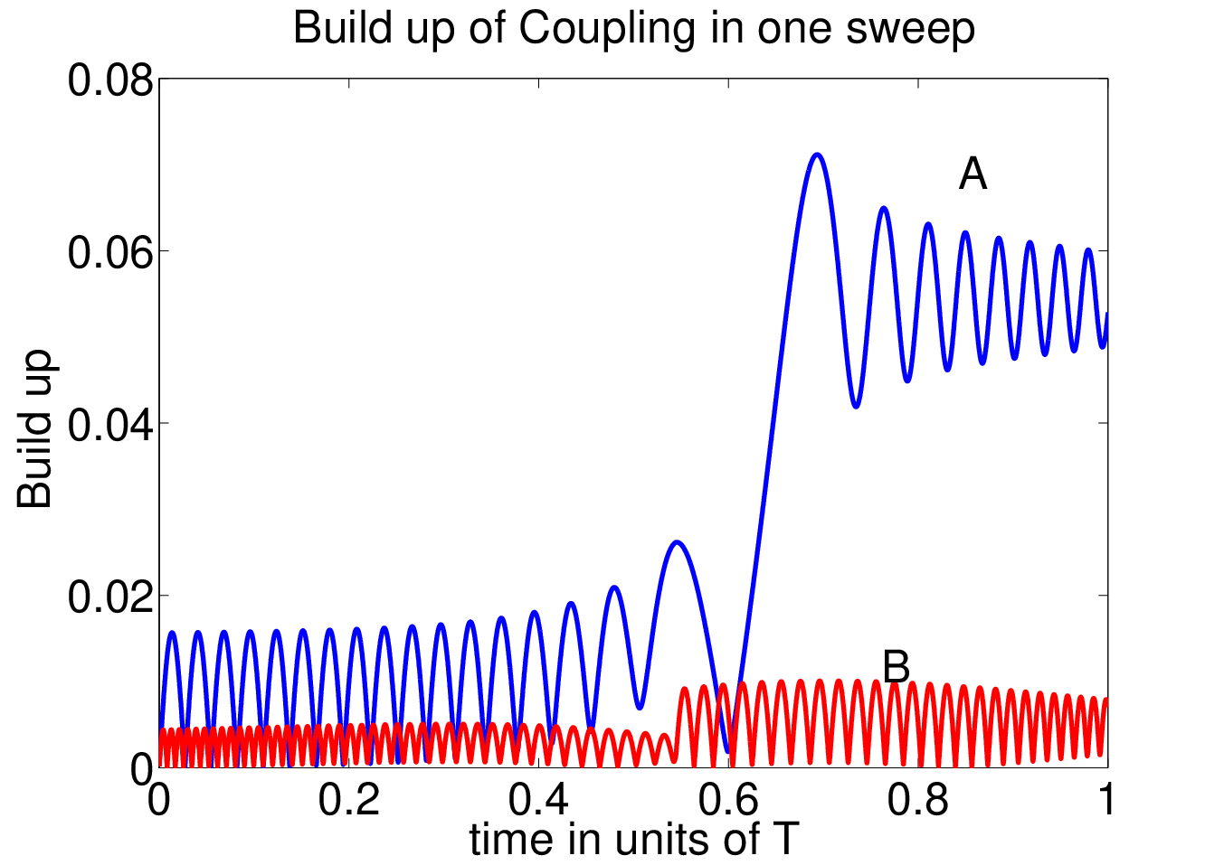
In Fig. 1a and 2, we choose kHz and kHz. Let kHz and kHz, Hz. We choose rf-field amplitude of kHz and a sweep rate , i.e., ( adiabaticity is well satisfied). The total time to sweep through is then ms. In Eq. 13, we have for , and . With these parameters, we plot in figure 3 (curve A) , the build up of zero quantum coupling Hamiltonian given by
| (14) |
in Eq. (13) in one period of chirp of duration . We see in we accumulate a coupling of strength around . To get a coupling of strength that transfers , we will need such periods, i.e. a duration of ms. For , this time is units of time. We also plot in figure 3 (curve B), build up of double quantum Hamiltonian. We find this is not much and hence terms in Eq. (13) are negligible. Further observe the build up of zero quantum coupling Hamiltonian happens when we sweep in the middle of the two resonances. In present simulation center of the resonances is at kHz and we sweep it at time , which is where we see the build up in figure 3 (curve A). Since double quantum terms in the Hamiltonian are rotated at sum of the effective frequencies , they always average out as shown.
In figure 3, we plotted build up of coupling in Eq. (9) of one period of chirp. We can also plot build up of coupling in Eq. (10) in two periods of chirp. This is not simple sum of two , there is a phase shift when we add effective coupling Hamiltonians in first period and second period as in Eq. (10). Because of this phase shift we find our transfer efficiency decreases and as shown in simulations below (see Fig. 4), it takes more than for the complete transfer in the pair kHz. We plot in Fig. 4 for different resonance pairs, the build up of transfer as function of mixing time, when we do many cycles of chirp and use the supercycle as described in Eq. (12). Recall a zero quantum Hamiltonian transfer and hence transfers . Our chirp mixing builds a zero quantum Hamiltonian for the transfer.

In Fig. 5 (left panel), we plot maximum transfer efficiency within time , as a function of resonance offsets . We plot a contour plot, showing a large high intensity plateau around diagonal, which signifies chirp mixing is very broadband. We do the same for state of the art DIPSI mixing (right panel) [18]. We find high intensity region around diagonal is much narrow. We find chirp mixing is much broader than DIPSI mixing.
 |
 |
3.2 Experimental
The chirp mixing pulse sequence was applied for 13C mixing in uniformly labelled amino acid Alanine. The molecule has three 13C resonances of Cβ, Cα and CO at ppm respectively with coupling Hz and Hz. All experiments were performed at magnetic field corresponding to 750 MHz proton frequency. The chirp mixing pulse sequence used for the experiments is the one defined in simulation section. We put the carrier half way between the resonances at 100 ppm. To find a good mixing time for the experiment, we first do a 1D experiment, where by use of gradients and selective pulses, the magnetization on Cα and CO is dephased. Then supercycles of chirp mixing are applied (each supercycle takes time ms) and we observe build up of magnetization on Cα starting from magnetization on Cβ. is incremented in units of and we plot the build up in Fig. 6. We find we get best transfer at . This correspond to a mixing time of ms. With this mixing time we do a 2D experiment, results of which are shown in Fig. 7. The carrier is at ppm. We collect 1024 points in indirect and 4096 points in the direct dimension. We use TPPI for data acquisition. During mixing proton is decoupled with a decoupling pulse sequence. We can see Cβ-Cα (a) , Cα-CO (b) and Cβ-CO cross peaks in Fig. 7.


4 Conclusion
In this paper, we developed the theory of chirp mixing. The pulse sequence for chirp mixing is simple, given coupled homonuclear spins with offsets in range , we adiabatically sweep through the resonances. This achieves cross polarization between the magnetization of the coupled spins. We repeat this adiabatic sweep for appropriate mixing time, with a supercycle. When we sweep midway between the resonances of the coupled spin and , the effective field seen by two spins is the same and hence they precess at same frequency around their effective fields. This means the coupling, which normally gets averaged due to the chemical shift difference is no more averaged and we get mixing. By virtue of its design, the chirp mixing is much more broadband compared to state of the art methods. We compared the performance of chirp mixing to DIPSI mixing. We find for a rf-field amplitude of kHz, DIPSI is only effective in a offset range kHz, while chirp mixing easily covers the range kHz and beyond. This range can be further extended, by increasing the sweep width.
The proposed methodology was demonstrated on 13C mixing in a sample of Alanine. We anticipate the proposed methods will soon find applications in broadband 13C mixing in protein NMR spectroscopy at high fields. At field strengths of GHz the 13C spectrum is spread over a kHz range, which can be easily covered with chirp mixing with moderate rf-field strengths of kHz.
References
- [1] J. Cavanagh, W. J. Fairbrother, A. J. Palmer and N. J. Slelton Protein NMR Spectroscopy, principles and practice, Academic Press, (1996).
- [2] L. Braunschweiler and R. R. Ernst, J. Magn. Reson. 53, 521-528 (1983).
- [3] L. Müller and R.R. Ernst, Mol. Phys.38, 963-992 (1979).
- [4] A. Bax and D. G. Davis, J. Magn. Reson. 65, 355-360 (1985).
- [5] D. G. Davis and A. Bax, J. Am. chem. Soc. 107 2820 (1985).
- [6] D. G. Davis and A. Bax, J. Am. chem. Soc. 107 7197 (1985).
- [7] J.S. Waugh, J. Magn. Reson. 68 189 (1986).
- [8] M. Rance, J. Magn. Reson. 74 557 (1987).
- [9] S. Subrumanian and A. Bax, J. Magn. Reson. 71 325 (1987).
- [10] R. Bazzo and J. Boyd, J. Magn. Reson. 75 452 (1987).
- [11] R. Bazzo and I. D. Campbell, J. Magn. Reson. 76 368 (1988).
- [12] N. Sunitha Bai and R. Ramachandran, J. Magn. Reson. A 105 298 (1993).
- [13] N. S. Rao and N. Reddy, Pramana J. Phys. 43 91 (1994).
- [14] S. J. Glaser and G.P. Drobny, Adv. Magn. Reson. 14 35 (1990).
- [15] A. J. Shaka, J. Keeler, and R. Freeman, J. Magn. Reson. 53, 313-340 (1983).
- [16] A. J. Shaka, J. Keeler, T. Frenkiel, and R. Freeman, J. Magn. Reson. 52, 335-338 (1983).
- [17] A. J. Shaka, C. J. Lee, and A. Pines. J. Magn. Reson. 77, 274-293 (1988).
- [18] S. P. Rucker and A. J. Shaka, Mol. Phys.68, 509-517 (1989).
- [19] M Kadkhodaie, O Rivas, M Tan, A Mohebbi, A.J Shaka. J. Magn. Reson. 91, 437-443 (1991).
- [20] P. Coote, H. Arthanari, T. Y. Yu, A. Natarajan, G. Wagner and N. Khaneja, J. Biomol NMR. 55(3) 291-302 (2013).
- [21] S. J. Glaser and J. J. Quant, Advances in Magnetic and Optical Reson. 19, 59-252 (1996)