Quantum fluctuation theorems for arbitrary environments:
adiabatic and non-adiabatic entropy production
Abstract
We analyze the production of entropy along non-equilibrium processes in quantum systems coupled to generic environments. First, we show that the entropy production due to final measurements and the loss of correlations obeys a fluctuation theorem in detailed and integral forms. Second, we discuss the decomposition of the entropy production into two positive contributions, adiabatic and non-adiabatic, based on the existence of invariant states of the local dynamics. Fluctuation theorems for both contributions hold only for evolutions verifying a specific condition of quantum origin. We illustrate our results with three relevant examples of quantum thermodynamic processes far from equilibrium.
pacs
05.70.Ln, 05.40.-a 05.70.-aI Introduction
Classical thermodynamics and statistical mechanics provide a systematic approach to the phenomenology of a system immersed in a large environment. Within these frameworks, two complementary strategies are employed. The first is to explicitly model the environment —often an equilibrium thermal reservoir— to obtain an effective reduced dynamics for the system alone, which then can be analyzed. The second is to derive fundamental constraints in the form of inequalities using the second law of thermodynamics and magnitudes like entropy, entropy production and free energy. The recent introduction of an entropy for stochastic trajectories [1] allows one to refine these inequalities with exact equalities for arbitrary nonequilibrium processes, results generically known as fluctuation theorems (FT’s) [2, 3].
These two strategies have also been successfully applied to quantum systems. Open quantum system dynamics —the determination and analysis of the system’s reduced dynamics— is a well-developed and active field [4, 5]. Complementing this approach, a variety of quantum FT’s have been derived [6, 7, 8, 9, 10, 11] to asses the statistics of the relevant quantities. Different proposals to obtain these statistics in the laboratory have been reported, using techniques related to quantum tomography [12, 13, 14, 15, 16, 17], and some of them have already been used to carry out experimental verifications of FT’s [18, 19]. However, most of the research on quantum FT’s is only valid for equilibrium reservoirs with a focus on the energy exchange between the system and the environment in the form of heat and work. By contrast, classical FT’s have been formulated more generally for generic Markov systems [20, 21, 22, 23, 24] using the entropy production instead of heat and work, which are only meaningful in physical situations where a system exchanges energy with equilibrium reservoirs.
In light of the success of classical FT’s, it is desirable to obtain complementary FT’s for generic quantum dynamics [25, 26, 27, 28, 29, 30, 31, 32, 33, 34, 35]. They could be of particular relevance, since quantum mechanics allows for a richer phenomenology in finite baths [36, 37, 38], as well as novel and interesting non-thermal environments such as coherent [39, 40], correlated [41], or squeezed [42, 43, 44, 45] reservoirs. Such environments induce an interesting phenomenology that goes beyond the thermodynamics of thermal equilibrium reservoirs, such as heat engines that outperform Carnot efficiency [46] and may exhibit new regimes of operation [45, 47] or tighter bounds on Landauer’s principle [48, 49].
The task of deriving FT’s for generic quantum dynamics also implies a more detailed characterization of entropy production in nonequilibrium quantum contexts, a problem that has attracted a growing interest in recent years [50, 8, 51, 31, 52, 53, 30, 33, 54, 55, 56, 57]. In Ref. [33] we derived a FT for a class of completely-positive trace-preserving (CPTP) quantum maps, which model a variety of quantum processes. Through this analysis, we identified a quantity that coincides with the entropy production for thermalization processes and resembles the nonadiabatic entropy production introduced in the classical context [21, 22, 23]. The purpose of this paper is to clarify and extend those results considering together the system and its surroundings. By tracing over the environment, we can then recover the quantum map for the reduced system dynamics. This setup allows us to unveil the origin of entropy production in arbitrary processes from coarse-graining, and derive corresponding FT’s. We also split the entropy production into an adiabatic and a nonadiabatic contribution, exactly as in classical stochastic thermodynamics. However, contrary to what happens in classical systems, the split is not always possible. A condition, derived in Ref. [33], is necessary. We will explore the similarities and differences between classical and quantum FT’s in concrete examples.
The paper is organized as follows. In Section II, we introduce a thermodynamic process for a generic bipartite system that models a system and its environment. We will define in this section the entropy production along the process and the concomitant reduced system dynamics. We develop a FT for this entropy production in Section III using a time-reversed or backward thermodynamic process. In Section IV, FT’s for the adiabatic and nonadiabatic entropy production are derived. Our results are also extended both to the case of concatenations of CPTP maps and multipartite environments. This is applied to the specific case of quantum trajectories unraveled from Lindblad Master Equations in V. Finally, relevant examples to illustrate our results are given in Section VI while concluding in Section VII with some final remarks.
II Quantum operations and entropy production
Along the paper we consider an isolated quantum system composed of two parts, system and environment (or ancilla), with Hilbert space , where and are the local Hilbert spaces of the system and the environment respectively. We focus our attention on the entropy production along the generic process depicted in Fig. 1, consisting of initial and final local projective measurements that bracket a unitary evolution. The outcomes of the measurements constitute a quantum trajectory, which plays a crucial role in the formulation of FT’s.
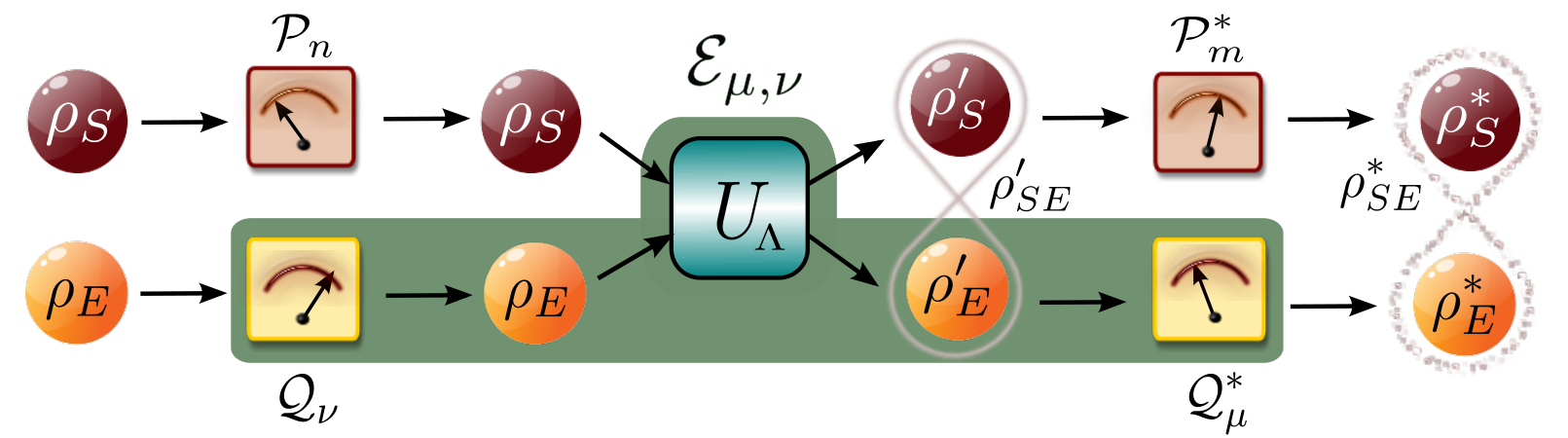
II.1 The (forward) process
The process begins with the global system in an uncorrelated product state . The spectral decomposition of the local states reads
| (1) |
where and are the eigenvalues, and and are orthogonal projectors onto their respective eigen-subpaces (for simplicity we assume they are rank-1 projectors).
At an initial projective measurement on the system and environment is performed using the eigenprojectors in Eq. (1) and outcomes and are obtained. This measurement projects the system and environment onto pure states and , without modifying the average or unconditional state of the global system ().
Subsequently, we evolve the compound system during the time interval . The corresponding unitary operator is generated by the Hamiltonian , which depends on time through an external parameter that we vary according to a prescribed protocol :
| (2) |
where denotes the time-ordering operator. As a result, the compound system at time is described by the new density matrix
| (3) |
which in general contains classical and quantum correlations. The reduced (or local) states of the system and the environment can be obtained by partial tracing: and .
To complete the process, a second local projective measurement is performed at time on both the system and environment. The measurement operators are arbitrary (rank-1) orthogonal projectors, denoted as and . Unlike in the first measurement, in this case the average global state is disturbed, transforming into
| (4) |
Notice also that this is not a product state: the final local measurement does not eliminate the classical correlations contained in [58]. However, the measurement collapses the local states of the system and environment into pure states and . Thus, the spectral decomposition of the reduced states after the final measurement is
| (5) | ||||
| (6) |
where and are the corresponding classical marginal distributions.
II.2 Reduced dynamics: maps and operations
The global manipulation described above induces a reduced dynamics on the system alone. The shaded area in Fig. 1 can be considered as an effective transformation of the state of the system, , described by the action of a quantum CPTP map that admits a Kraus representation [59]
| (7) |
with a set of Kraus operators satisfying .
There exist many Kraus representations that reproduce the reduced dynamics on the system. We choose
| (8) |
This specific representation retains all the details of the evolution of the environment, relating unequivocally each Kraus operator with a transition in the environment. This is a key point in order to characterize the thermodynamics of the process at the trajectory level, as we will see shortly. Let us finally define the quantum operation:
| (9) |
which describes the conditioned evolution of the system when the environment starts in the pure state and ends in the state after measurement [60].
II.3 Average entropy production
We now discuss the entropy change along the process. We analyze here the von Neumann entropy, of the global system. Recall that the von Neumann entropy coincides with the thermodynamic entropy for equilibrium states (setting the Boltzmann constant ). For non-equilibrium states there are some situations where the von Neumann entropy still can be interpreted as a thermodynamic entropy [61]. However, in this paper we will refrain from identifying with a thermodynamic entropy and refer to it simply as the entropy or the quantum entropy of state .
Along the process described above, the quantum entropy of the global system changes as
| (10) |
This quantity is the quantum entropy production along the process. We will refer to as the inclusive entropy production to distinguish it from the entropy production when the system and the environment are separated at the end of the process and the final classical correlations are lost (see below). The inclusive entropy production is always non-negative, since von Neumann entropy cannot decrease in a projective measurement and stays constant along any unitary evolution, i.e., . Notice also that equals the classical Shannon entropy of the probability distribution of pure states in the eigenbasis of . In particular we have
| (11) | ||||
| (12) |
To express the entropy of the global state in terms of local entropies and correlations, one can use the mutual information. For an arbitrary state with reduced states and , the mutual information is defined as
| (13) |
Here we have introduced the quantum relative entropy, , a non-symmetric and non-negative measure of the distinguishability between states and , which vanishes if and only if [62]. This property implies that mutual information becomes zero only for product (uncorrelated) states . Using mutual information, the inclusive entropy production can be rewritten as:
| (14) |
where we have taken into account that the initial state is uncorrelated and, therefore, . The second equality shows that there are two sources of entropy production. The first one is the measurement disturbance of the final local states and , which can be avoided only by measuring in the eigenbasis of the reduced states and . The second source, captured by the term , is the erasure of quantum correlations in the state . This is due to the local character of the measurements, being zero only if the global interaction does not generate quantum correlations [63, 64].
In most situations the classical correlations remaining after the final measurement are irreversibly lost, with an entropic cost equal to the mutual information . This is the case if we separate system and environment after the process and all subsequent manipulations are local and do not incorporate any feedback based on the outcomes of the final measurements. The entropy production in those situations is
| (15) |
We will refer to as the non-inclusive entropy production or simply entropy production. The positivity of the non-inclusive entropy production in Eq. (15) has been already identified with the second law [48] and the existence of a thermodynamic arrow of time [65, 66]. Notice that , since the mutual information is always non-negative.
The differences between inclusive and non-inclusive entropy production will be illustrated in a specific example in Sec. VI.1.
III Backward process and fluctuation theorem for the entropy production
III.1 Forward and backward trajectories
We now extend the previous analysis to stochastic entropy changes at the level of individual quantum trajectories. A trajectory of the process introduced in the previous section (hereafter, we will call it the forward process) is simply given by the outcome of the four measurements, i.e., . This trajectory corresponds to the following transition between pure states
| (16) |
Notice that, in virtue of our choice of the Kraus representation for the reduced dynamics [Eq. (8)], a trajectory is also a trajectory of the reduced dynamics, where the pair now indicates the Kraus operation affecting the system instead of the initial and final states of the environment (which is otherwise hidden in the reduced dynamics). The probability to observe that trajectory is given by
| (17) |
To introduce the backward process, we make use of the anti-unitary time-reversal operator in quantum mechanics, , satisfying and . This operator changes the sign of odd variables under time reversal, like linear and angular momenta or magnetic fields [6, 67]. We will consider the separate time reversal operators for system, , and environment, , as well as the one for the total bipartite system .
The backward process is defined as follows. We start with a generic initial state of the form
| (18) |
As in the forward process, the first step at time is a local measurement of the family of projectors . According to Eq. (18), the outcomes and are obtained with probability . We then let the global system evolve under the Hamiltonian inverting the time-dependent protocol as with . This evolution is given by the unitary transformation
| (19) |
Finally, at time we perform new local measurements on the system and environment using projectors . The outcome induces a quantum jump
| (20) |
and the corresponding backward trajectory occurs with probability
| (21) |
III.2 Fluctuation theorem
The unitary transformations corresponding to the forward and the backward process satisfy the so-called micro-freversibility principle for non-autonomous systems [68, 6]:
| (22) |
This is the key property that relates the probabilities of trajectories and in a quantum FT. By comparing the probabilities (17) and (21), using micro-reversibility (22) and the cyclic property of the trace, we immediately get
| (23) |
where we have defined the quantities
| (24) | ||||
| (25) |
The terms in Eq. (24) are related to entropy changes per trajectory in the system and the environment, whereas in Eq. (25) corresponds to the stochastic version of the mutual information [69, 25] in the initial state of the backward process (18). From the detailed FT in Eq. (23), we immediately have the integral version
| (26) |
and, using Jensen’s inequality , one obtains a second-law-like expression .
The interpretation of depends on the choice of , the initial global state of the backward process. If we set , then and becomes the inclusive entropy production per trajectory. Its average
| (27) | |||||
equals the inclusive entropy production defined in Eq. (10). If the initial condition for the backward process is the uncorrelated state , then and is the non-inclusive entropy production per trajectory, whose average yields the entropy production defined in Eq. (15)
| (28) |
A third choice sets the environment in the (inverted) initial state of the forward process, , which yields . In this case both initial and final local measurements in the environment are performed in the same basis , and we obtain
| (29) |
which includes an extra contribution measuring the disturbance on the environment during the process. The term , unlike , is negligible when the environmental state is modified only infinitesimally (see appendix A), as is the case e.g. of a large reservoir. Moreover, when is a Gibbs state, Eq. (29) is the entropy production proposed in Ref. [50], and corresponds to the thermodynamic entropy production due to irreversibly reseting the ancilla back to in contact with an equilibrium reservoir at the same temperature. Finally, we stress that for equilibrium canonical initial conditions both in the forward and in the backward processes, the trajectory entropy production (23) equals the stochastic dissipative work and one recovers the celebrated Crooks work theorem and the original Jarzynski equality [6, 7].
IV Dual processes: adiabatic and non-adiabatic entropy production
We now focus on the reduced dynamics. Our aim is to obtain FT’s involving only the quantum trajectory defined in Sec. III and the initial and final states of the system. To do that, we follow our previous work [33], where we derived a FT for CPTP maps based on the dual dynamics introduced by Crooks in Ref. [70]. Remarkably, the resulting FT goes beyond the one that we have obtained considering the global dynamics, Eq. (23), as it will reveal an interesting split of the total entropy production into two terms: the adiabatic entropy production, which accounts for the irreversibility of the stationary regime, and the non-adiabatic entropy production, which measures how far the system is from that stationary state.
We apply the formalism in Ref. [33] to , the map governing the reduced dynamics of the process, as well as to the map corresponding to the backward dynamics. Therefore, we first need to introduce the reduced dynamics in the backward process, which will be described by a new CPTP map . To do that, it is necessary that the system and the environment start the backward process in an uncorrelated state , i.e., we have to impose [see Eq. (25)]. Otherwise the CPTP map of the backward reduced dynamics would depend on the initial state of the system. In that case, similarly to our choice (8) for the forward process, a useful representation of is
| (30) |
where the backward Kraus operators are given by
| (31) |
Notice that here we have swapped subscripts with respect to the definition of the forward operators given by Eq. (8). This can be done since the pair is just a label of the Kraus operator. The choice in Eq. (31) means that the operation is equivalent to obtaining in the initial measurement of the backward process and in the final one. Now, micro-reversibility (22) implies an intimate relationship between the forward and backward Kraus operators:
| (32) |
It is important to notice that the FT for the total entropy production (23) can be derived directly from the above equation. In other words, Eq. (32) expresses the fundamental symmetry under time reversal yielding the FT.
IV.1 The dual-reverse process and non-adiabatic entropy production FT
In order to go beyond the FT for the total entropy production, we proceed as in Refs. [70, 33]. These works, inspired by classical stochastic thermodynamics, introduce a quantum dual dynamics that reveals the irreversibility associated to a map at the steady state. In the following we denote an invariant state of the forward map, , which we indeed assume to be positive definite. The dual dynamics, which we will call here dual-reverse following the criterion used for classical systems [21, 22, 23], is defined as a map such that is an invariant state, i.e., . Furthermore, when the map is applied several times starting from the stationary state , it generates trajectories distributed as . Here the trajectories are and , corresponding to applications of the map.
Summarizing, in the stationary regime the dual-reverse generates the same ensemble of trajectories as the forward process, but reversed in time. For instance, if the map describes the dynamics of a system in contact with a single thermal bath (thermalization), then the forward process generates reversible trajectories (indistinguishable from their reversal) and the dual-reverse coincides with the forward map. In nonequilibrium situations, the dual generically inverts flows. For instance, for a system in contact with two thermal baths at different temperatures, the dual-reverse is usually obtained by swapping the temperatures of the baths, hence inverting the flow of heat.
In any case, one can prove that a Kraus representation of the dual-reverse map is given by the operators [70, 33]:
| (33) |
Finally, the dual-reverse process is the dual-reverse map complemented by a specific choice of the initial condition for the system (the environment does not appear explicitly in the dual map, which acts only on the system). The appropriate initial condition for the dual-reverse process is , i.e., the same as the backward process.
We now have three processes: the forward , the backward , and the dual-reverse , each one inducing an evolution in the system characterized by trajectories . We can compute the probability of observing a trajectory or its reverse in each of those evolutions. With a self-explanatory notation, these probabilities read
| (34) | |||||
| (35) | |||||
| (36) |
To obtain FT’s from these expressions we need a condition of proportionality between operators , and , similar to the relationship (32) between and .
In [33] inspired by [71], we found that a necessary and sufficient condition for that proportionality is the following. We first define the nonequilibrium potential , from the invariant state . Its spectral decomposition reads:
| (37) |
where , and and are, respectively, the eigenvalues and eigenstates of the invariant density matrix . Now we require that each Kraus operator is unambiguously related to a nonequilibrium potential change (note however that the converse statement is not necessarily true, i.e. we may have for different values of and the same value of ). In the invariant state eigenbasis this condition reads:
| (38) |
with whenever . As pointed in [33], this condition does not imply single jumps between pairs of eigenstates, but it could account for any set of correlated transitions between different pairs with same associated . An extreme example are unital maps, where is proportional to the identity matrix. In that case, and any complex coefficients satisfy Eq. (38). It is not hard to show that condition (38) is equivalent to [33]
| (39) |
This alternative formulation of (38) indicates that, when , can be interpreted as ladder operators in the eigenbasis of the invariant state .
For thermalization or Gibbs preserving maps, with , being the inverse temperature and the equilibrium free energy, the potential is and is the energy transfer between the system and the environment, i.e., the heat. Condition (38) in this case implies that the Kraus operators produce jumps between levels with the same energy spacing or, equivalently, jumps with a well defined value of the heat.
Introducing condition (38) in Eq. (33), one easily derives the following relationship between the forward and the dual-reverse Kraus operators [33]:
| (40) |
and, using Eq. (32), one gets:
| (41) |
Finally, inserting (40) and (41) into the expressions for the probability of trajectories (34-36) we obtain the following FT’s:
| (42) | |||||
| (43) |
We will call the adiabatic entropy production and the non-adiabatic entropy production, following the terminology used in classical stochastic thermodynamics [21, 22, 23]. They contribute to the total entropy production per trajectory, , as defined in Eq. (23). Below we discuss the averages of the adiabatic and non-adiabatic entropy production in some cases, clarifying the origin of the terms.
IV.2 The dual process and adiabatic entropy production FT
Notice that (43) is not a proper FT for the forward process. In particular, we cannot derive a Jarzynski-like equality for averaged over forward trajectories, . To achieve this goal we need a further assumption that will allow us to apply the results of Ref. [33] to the backward process. In this way, we will obtain the dual-reverse of the backward process, which we simply call the dual map . If condition (38) is satisfied, then, by virtue of (32), the backward Kraus operators can be written as:
| (44) |
with . We observe that, setting , condition (38) is recovered for the backward process. However, a requirement to apply the theoretical framework developed in Ref. [33] is that is an invariant state of the backward map . This is not warranted by the definition of , not even when the Kraus operators are of the form (38). Therefore, we have to add this extra assumption. In particular, it is satisfied when the driving protocol associated to the map is time-symmetric, the Hamiltonian of the environment is invariant under time reversal, and we perform the same measurements at the beginning and the end of the process on the environment. This is the case of the infinitesimal maps that govern the dynamics of a quantum Markov process since, even in the case of arbitrary driving, each map is generated by a constant Hamiltonian.
We now obtain the dual operators , applying transformation (33) to the backward Kraus operators (with the role of and swapped [33]). Similarly to (40), condition (38) on the backward operators imply
| (45) |
and, using Eq. (32),
| (46) |
The dual process is given by the dual map with initial condition . The trajectories generated by this process are distributed as
| (47) |
IV.3 Integral fluctuation theorems
We can now derive integral FT’s for the adiabatic and non-adiabatic entropy productions:
| (49) |
which follow from the detailed versions by averaging over trajectories . Finally, convexity of the exponential function provides the following two second-law-like inequalities as a corollary and . As for the FT for the total entropy production (23), the meaning of these average entropies becomes clearer if the initial condition of the backward process is specified. Setting , the average of the adiabatic and non-adiabatic entropy production defined by (40) and (41) reads
| (50) | |||||
| (51) |
and the sum equals the total non-inclusive average entropy production [see Eq. (15)]. It is interesting to notice that the average change of the potential,
| (52) |
can be alternatively written in terms of averages over the states of the system, and if condition (38) is fulfilled. That condition implies (see also Ref. [33]). Introducing the commutator in (52),
| (53) |
where we have used the cyclic property of the trace and Eqs. (7) and (8). Therefore, the average potential change can be expressed as the change in the expected value of the operator due to the map. Recall that the operator acts on the Hilbert space of the system , i.e., is a local observable on the system.
If the final measurement does not alter the state of the system, i.e., if , or if the final measurement is skipped, as it is the case when we concatenate maps and the system is measured only after the whole concatenation (see Sec. IV.5 below), we can write the average non-adiabatic entropy production in an appealing form:
| (54) |
where we have used the definition of the potential operator in terms of the invariant state . Here we see that the non-adiabatic entropy production is related to the distance between the state of the system and the invariant state . During the evolution, the state of the system can only approximate the invariant state and the non-adiabatic entropy production is a measure of the irreversibility associated to such convergence. In fact, inequality in Eq. (54) follows from direct application of Ulhman’s inequality (monotonicity of quantum relative entropy) holding for general CPTP evolutions [62, 51].
IV.4 Multipartite environments
The results obtained so far can be also applied to multipartite environment. The corresponding Hilbert space is decomposed as , corresponding to independent ancillas or reservoirs interacting with the open system. We assume an uncorrelated initial state of the environment, , and that the measurements are performed locally in each environmental ancilla.
In this case the adiabatic entropy production per trajectory and its average read (see details in appendix B):
| (55) | |||||
| (56) |
IV.5 Concatenation of CPTP maps
Up to now, we have considered a single interaction of duration between the system and the environment [see Eq. (2)]. The CPTP map describes the evolution of the system when the environment is measured before and after interaction. This framework can be extended to concatenations of CPTP maps, where the system interacts sequentially with the environment. Each single interaction in an time interval is described by a single CPTP map like . The map describing the reduced dynamical evolution for interactions, from to , is:
| (57) |
where, in particular, each map may have a different (positive-definite) invariant state . We assume that the system interacts from time to time with a “fresh” (uncorrelated) environment in a generic state , and, as in the single map case, the environment is measured before and after interaction with the system by projective measurements. On the other hand, the system is only measured at the beginning and end of the the whole concatenation (57), as depicted in Fig. 2.

In this case, trajectories are specified by the set of outcomes , which can be compared to the backward trajectories generated by the reverse sequence of maps . We find that all our above results apply as well to the concatenations setup (see appendix C) yielding the following three detailed fluctuation theorems:
| (58) | |||||
| (59) | |||||
| (60) |
where is given by Eq. (24), is the entropy change in the environment due to the -th map, and is the change in non-equilibrium potential for the -th map.
V Lindblad Master Equations
The results of the last section can be applied to Lindblad master equations [31, 52]. Consider the following master equation in Lindblad form [4, 60, 72], depending on an external parameter :
| (61) |
where is the system Hamiltonian in the selected picture and are positive Lindblad operators, which generally depend on the control parameter and describe jumps in some (possibly time-dependent) basis. We assume that there exists an instantaneous invariant state , which is the steady state of Eq. (61) when the external control parameter is frozen: [5].
The Lindblad equation (61) can be written as a concatenation of CPTP maps
| (62) |
with the Kraus representation
| (63) | |||||
| (64) |
Recall that this Kraus representation is not unique [60]. As before, the representation (63-64) is related to a specific detection scheme for the jumps, that is, it implies a specific choice of the initial state and the local observables to be monitored in the environment (the set of projectors and ).
The Kraus representation (63-64) is based on a family of operations with that induce jumps in the state of the system and occur with probabilities of order , and a single operation that induces a smooth nonunitary evolution and occurs with probability of order 1. This implies that a trajectory consists of a large number of 0’s punctuated by a few jumps with . An alternative way of describing the trajectory is to specify the jumps and the times where they occur, i.e., , where, as before, and denote the outcomes of the initial and final measurements in the system at times and . Jump is given by the operation , whereas between two consecutive jumps at and the evolution is given by the repeated application of the operation corresponding to the Kraus operator in (63). This results in a smooth evolution given by the operator:
| (65) |
with an effective non-hermitian Hamiltonian that reads
| (66) |
In this representation, the probability of a trajectory is
| (67) |
with .
V.1 Backward, dual and dual-reverse dynamics
Consider now the backward dynamics. The time-inversion of the evolution of the global system corresponds to a time-reversed version of the Lindblad master equation (61). As in the previous section, the backward process is generated by inverting the sequence of operations together with time-inversion of each operation in the sequence. The map corresponding to an infinitesimal time-step in the time-reversed dynamics, , admits a Kraus representation with Kraus operators . To obtain the backward map, we would need to know details about the environment that induces the Markovian dynamics given by the Lindblad equation (61). However, in the previous sections we have derived a relationship between the forward and backward CPTP maps, namely Eq. (32):
| (68) | ||||
| (69) |
Imposing the backward maps to be trace-preserving, that is, , we obtain , and the consistency condition
| (70) |
Any set of numbers satisfying Eq. (70) defines, through (68), an admissible backward process. The existence of such set is warranted, since any Lindblad equation can be derived from the interaction between the system and an ancilla.
For any trajectory generated in the forward process with probability , there exist a backward trajectory occurring in the backward process with probability . The backward trajectory can also be identified by the times of successive jumps. In this representation, the probability of trajectory can be written as:
| (71) |
where . The smooth evolution between jumps is given by the operator
| (72) |
where again corresponds to the inverse sequence of values for the control parameter. It can be shown that this smooth evolution obeys the micro-reversibility relationship .
Let us discuss now the dual and dual-reverse dynamics. The condition (39), necessary to define the dual-reverse process, reads [31, 52]:
| (73) |
These commutation relationships indicate that the Lindblad operators promote jumps between the eigenstates of . Furthermore, as the condition must be fulfilled for the operator in Eq. (63) as well, we need , which in turn implies . This means that the instantaneous steady state of the dynamics must be diagonal in the basis of the Hamiltonian term appearing in Eq. (61). This condition is fulfilled by equilibrium Lindblad equations and in situations in which the operator becomes the identity operator in an appropriate interaction picture (see e.g. Refs. [45, 73]). However, the condition can be broken in nonequilibrium situations, a genuine quantum effect. In section VI.3 we present an example of a periodically driven cavity mode where the adiabatic entropy production can be negative. Finally, as discussed in section IV.2, we recall that the fluctuation theorem for the adiabatic entropy production can be stated when the backward maps admits as an invariant state.
If these conditions are fulfilled, the dual process is defined by the dual operations with Kraus operators as defined in Eq. (46), whereas the dual-reverse process is given by operations with Kraus operators defined in Eq. (40) (see also Eqs. (148-149) in App. C). The probability of a trajectory in the dual process, , can be calculated from Eq. (67) by using the same map for the no-jump time evolution intervals, and replacing the operations by the dual operations . Analogously, for the dual-reverse process the probability of trajectory , , can be constructed from Eq. (71) with for the no-jump evolution, and dual-reverse operations . We further notice that in general , and , that is, .
In many applications, the Lindblad operators come in pairs and the corresponding pair of terms in the sum (70) cancel. That occurs if, for a specific pair of operators , we have and , and being positive transition rates, and some arbitrary (possibly time-dependent) system operator. Then, condition (70) implies (cf. [74])
| (74) | ||||
and the (inverted) Kraus operators of the backward map are also operators of the forward map:
| (75) |
where we have used the detailed-balance relation (32). Moreover, is invariant under the backward map:
| (76) |
V.2 Entropy production rates
The above considerations lead us to reproduce the three different detailed FT’s in Eqs. (60) for quantum trajectories generated by Lindblad master equations. From the integral fluctuation theorems we can derive second-law-like inequalities analogous to Eqs. (50) and (51) for the entropy production rates [31]:
| (77) | ||||
| (78) |
where is the derivative of the von Neumann entropy of the system, is the nonequilibrium potential change rate, and the entropy change in the monitored environment during [52]. The three above equations guarantee the monotonicity of the average entropy production, , and the adiabatic and non-adiabatic contributions, and , during the whole evolution.
The physical interpretation of the adiabatic and non-adiabatic entropy production now becomes clear. The non-adiabatic part can be written as
| (79) |
which is the continuous time version of Eq. (54). If the control parameter changes quasi-statically, we have and, therefore, the non-adiabatic entropy production vanishes. This is analogous to the classical non-adiabatic entropy production introduced in Refs. [20, 21, 22, 23]. On the other hand, the adiabatic contribution is in general different from zero even if the driving is extremely slow. In a physical system, this term accounts for the entropy production required to keep the system out of equilibrium when is fixed, and the associated dissipated energy is usually referred to as housekeeping heat [20].
At this point, it is worth it to remark an important difference between classical and quantum systems. In classical systems, the split of the entropy production in two terms, adiabatic and non-adiabatic, can always be done at the level of trajectories, and both terms obey fluctuations theorem that ensure the positivity of their respective averages. This is possible for quantum systems only if (39) [or (73) for Lindblad operators] is met. One can still use (79) as a definition for the average non-adiabatic entropy production and for the average adiabatic entropy production rate. However, these definitions cannot be extended to single trajectories and, furthermore, they do not obey a fluctuation theorem. In the next section, we discuss a specific example where the condition is not fulfilled and, as a consequence, the average adiabatic entropy production rate can be negative.
Finally, it is also important to notice that and in Eqs. (77) are exact differentials, i.e., can be written as the time derivative of the system and the environment entropy, respectively. On the other hand, the term , as well as the adiabatic and non-adiabatic entropy production rates in Eq. (78), cannot be expressed, in general, as a time derivative. One important exception is the case of a constant invariant state like, for instance, in a relaxation in the absence of driving. In that case, all the quantities in Eqs. (77-78) are exact differentials. In particular, the non-adiabatic entropy production when the system relaxes from to is given by
| (80) |
which equals for a full relaxation to . The later coincides with the entropy production introduced by Spohn [75].
VI Examples
We illustrate our findings with three paradigmatic examples. In the first one, we consider a two-qubit CNOT gate as a simple process with a finite size environment to illustrate the differences between the inclusive and non-inclusive entropy production introduced in section II.3. The second and third examples correspond to two representative examples of non-equilibrium quantum Markov systems. The second example is an autonomous system coupled to several thermal baths. In this case, the non-adiabatic entropy production is zero except during the transient relaxation to the steady state. However, it provides an intuitive picture of how entropy is produced in non-equilibrium setups. The third example is a driven system that does not fulfill condition (38) and, consequently, does not admit the splitting of the entropy into adiabatic and non-adiabatic contributions with positive averages.
VI.1 A two-qubit CNOT gate
The difference between the inclusive and non-inclusive entropy production introduced in section II.3 becomes especially relevant for processes where the system of interest repeatedly interacts with a finite-size reservoir. As an extreme case we consider both system and environment to be qubits with the same energy spacing . Their Hamiltonians are given by and . We assume the initial state of the system to be partially coherent, with , and the environmental qubit starting in a thermal state at inverse temperature , being the partition function. The initial state can be written as
| (81) |
where , with are the Pauli matrices, and we take the standard qubit basis for both the system and the environment. The eigenbasis of determines the projectors of the initial measurements , which are in this case with and with .
System and environment interact through a CNOT gate, , where the system acts as the control qubit [62]. The interaction leads to the following global system-environment state
| (82) | ||||
Notice that has maximally mixed reduced states both in system and environment. As a consequence, for any choice of the final projectors , we have . In contrast, the global state depends on the final projectors. The average work done during the interaction is , while there is no further energy contributions from local measurements.
The inclusive entropy production in Eq. (14) is just given by the erasure of quantum correlations in the final measurements, . This is the so-called mutual induced disturbance introduced by Luo [63]. Moreover if, following Refs. [76, 77], we maximize over , then the inclusive entropy production is equal to the (symmetric) quantum discord [78, 64] of the state . On the other hand, the non-inclusive entropy production in Eq. (15) is given by the total correlations in state , that is, , and it is independent of the choice of the local projectors of the final measurements .
The entropy production per trajectory can be calculated as explained in Sec. III. Recall that we may obtain both the inclusive or non-inclusive entropy production depending on our choice for the initial state of the backward process, and that the two quantities verify the integral fluctuation theorem (26).
In Fig. 3 we show the probability distribution of the entropy production for and . Blue solid bars correspond to the non-inclusive version and purple dashed bars correspond to the inclusive one. The latter does depend on the final measurements. Here we have taken as final projectors the local energy eigenbasis, for . The different types of average entropy production are plotted in the inset figure as functions of for the same value of . There, black and blue solid lines correspond to the average non-inclusive entropy production with and without including the term due to local disturbance of the environment [see Eq. (29)], respectively. Dashed and dotted lines show to the average inclusive entropy production for different choices of the local projectors in the final measurement . The purple dashed line is obtained when the final projectors are given by the local energy eigenbasis for . The orange dotted line is the symmetric quantum discord, obtained when maximizing .
As mentioned in section II.3, inclusive and non-inclusive entropy production apply to different physical situations depending on how the system and the environment are manipulated after the process. If system and environment are separated and every further manipulation is local, then we do not make use of the classical correlations given by the mutual information ; in this case the non-inclusive entropy production is the magnitude that adequately describes the increase of entropy. On the other hand, global operations on the whole system+environment can make use of those correlations and, for instance, extract more energy from a thermal bath. We illustrate this possibility in our simple example by considering a second CNOT interaction after the final local measurements. For simplicity we perform the final measurements in the local energy basis, for . Applying these projectors to state in Eq. (82), one obtains the final global state
| (83) |
Applying the second CNOT to this state, one gets
| (84) |
where is the initial thermal state of the environment. As we can see, in this second process system and environment become completely decorrelated after interaction, while a work is extracted when performing the second gate. Notice that the extracted work equals the work performed in the first gate. This work extraction is impossible if we only have local operations at our disposal, for which the final state is completely equivalent to the uncorrelated state .
This simple example highlights the importance of distinguishing between inclusive and non-inclusive entropy production in a small finite-size environment. Similar conclusions can be applied for the term .
VI.2 Autonomous thermal machine
Consider an autonomous three-level thermal machine powered by three thermal reservoirs at different temperatures, as depicted in Fig. 4 [79, 80, 44, 81, 82]. Each bath mediates a different transition between the energy levels, . The Hamiltonian of the system is
| (85) |
that is, the three possible transitions , and have frequency gaps , , and , respectively. Each transition is weakly coupled to a bosonic thermal reservoir in equilibrium at inverse temperature with , where we assume for concreteness.

The dynamics of the three-level thermal machine can be described by a Lindblad master equation obtained in the weak coupling limit by standard techniques from open quantum systems theory [4, 60, 5]. It reads
| (86) |
where is the density operator of the three level system and Lamb-Stark shifts have been neglected. The three dissipative terms in the above equation describe the irreversible dynamical contributions induced by each of the three thermal reservoirs:
| (87) |
where , and are the ladder operators of the three-level system. Equation (87) describes the emission and absorption of excitations of energy to or from the reservoir , at rates and , fulfilling detailed balance . Here is the mean number of excitations of energy in reservoir , and are the spontaneous emission decay rates associated to each transition. The heat fluxes entering from the reservoirs associated to the imbalance in emission and absorption can be defined as for , and the first law of thermodynamics reads .
Therefore, in our example we have six Lindblad operators ():
| (88) |
that define the infinitesimal CPTP map (62) with the Kraus representation given by Eqs. (63-64). In particular:
| (89) | ||||
| (90) |
Here the stochastic jumps during the evolution correspond to simple transitions between the energy levels . Therefore, the stochastic dynamics is completely equivalent to a classical Markov process if the initial state of the machine is diagonal in the Hamiltonian eigenbasis. In particular, the stationary state reads:
| (91) |
In appendix D, we explicitly calculate the occupation probabilities , , and . Nevertheless, the transient dynamics could exhibit some quantum effects when the initial state exhibit coherences in the Hamiltonian eigenbasis. For instance it has been recently pointed that initial coherence can be used to reach lower temperatures during the transient dynamics [83, 84].
The backward trajectory is defined by the inverse sequence of events with respect to , occurring in the backward process. We consider the initial state of the backward process the inverted final state of the forward process, , while the thermal reservoirs have the same state as in the forward process. We further assume the simplest form for the time inversion operator , namely, the complex conjugation, i.e., , which commutes with any matrix with real entries, as the Hamiltonian and the jump operators , .
The Lindblad operators in this case come in pairs . Hence the stochastic entropy change in the environment for each operator is given by Eq. (74), where the label takes on the six possible values and with :
| (92) |
This is as expected, since the upward jump induced by the operator in the forward trajectory dissipates a heat to the reservoir at inverse temperature . Equivalently, in the downward jump a heat is extracted from the thermal bath reducing its entropy by an amount . The Kraus operators of the backward map are given by Eq. (75): , and , and for the no-jump evolution. Indeed, by virtue of Eq. (72), we obtain for the effective evolution operator describing the dynamics between jumps in the backward process. From the above equations we see that the backward map is obtained from the forward map inverting the jumps. We also notice that, consequently, the backward map admits the time-reversed steady state as an invariant state.
We next construct the dual and dual-reverse processes for the model. The condition for the Lindblad operators to be of the form in Eq. (38) is fulfilled here. Indeed, the non-equilibrium potential, , obeys and
| (93) |
where the nonequilibrium potential changes associated to each jump in the trajectory read
| (94) |
Here we have introduced the quantities , and , which can be seen as the local inverse temperature (or virtual temperature [85, 86, 87]) of each transition in the steady state . As shown in appendix D, they determine the direction of the heat flow in the stationary regime, i.e., if , then the temperature of reservoir is higher than the local temperature of the machine and the heat is positive (energy flows from the reservoir to the machine), and viceversa. Moreover, for the heat flow is proportional to ; therefore, the difference can be considered as a thermodynamic force for the heat flow between the reservoir and the system. In Fig. 5 we plot the local inverse temperatures compared to the reservoir temperatures for a specific choice of and and as a function of , the inverse temperature of the coldest bath (we use units of ). There is a point, around , where and all the heat flows in the stationary regime vanish. Below that point, the steady heat flow from the coldest reservoir at inverse temperature is positive, i.e., the machine acts as a refrigerator that extract energy from the coldest bath 1. On the other hand, for , heat flows from the machine to the hottest bah at inverse temperature , so the machine acts as a heat pump capable to heat up the hottest reservoir 2.
The Kraus operators for dual and dual-reverse maps, and , can be obtained from Eqs. (46) and (41) respectively, by using Eqs. (92) and (94). They read:
| (95) | |||||
| (96) | |||||
| (97) | |||||
| (98) |
We see that the dual and dual-reversed dynamics induce similar jumps in the three-level system, but with modified rates depending on the differences . Only when for each , the dual process becomes equal to the forward process, and hence the dual-reverse process equals the backward process (see Fig. 5).
Notice that Eq. (93), together with the backward map having as an invariant state, are sufficient conditions to ensure the existence of the three fluctuation theorems for the adiabatic, non-adiabatic and total entropy productions during trajectory . They explicitly read:
| (99) | ||||
| (100) | ||||
| (101) |
where is the stochastic entropy increase in the system, and is the stochastic heat entering the system from reservoir , being the total number of upward or downward jumps in transition . The expression for the adiabatic entropy production is particularly interesting, since it is equal to the entropy generated by the heat transfer between reservoirs at inverse temperatures and . In particular, the adiabatic entropy production is identically zero when even though it is possible to have transient flows of heat.
We can now calculate the average rates of nonequilibrium potential and reservoirs entropy changes:
| (102) | |||||
| (103) |
where we split in three parts the nonequilibrium potential flow . The entropy production rates hence read:
| (104) | ||||
| (105) | ||||
| (106) |
showing the same structure as the trajectory entropies in Eqs. (99-101). Since there is no driving in this example, the non-adiabatic entropy production reads as in Eq. (80), and equals for a full relaxation to the steady state .
In the steady state we have , and the first law becomes . This implies that the only contribution to the entropy production rate is the adiabatic one, which can be written as:
| (107) |
This equation can be used to bound the efficiency of the machine in the different regimes of operation. For instance, the efficiency of the machine acting as a refrigerator is given by
| (108) |
where is the so-called Carnot efficiency of a refrigerator [85].
VI.3 Periodically driven cavity mode
Our third example consists of a single electromagnetic field mode with frequency in a microwave cavity with slight losses in one of the two mirrors. The losses of the cavity are produced by the weak coupling of the cavity mode to a bosonic thermal reservoir in equilibrium at inverse temperature . In addition, an external laser of the same frequency and weak intensity drives the cavity mode producing excitations. The Hamiltonian of the system can be expressed as consisting of two terms: the first one is the Hamiltonian of the undriven mode and
| (109) |
describes the effect of the classical resonant laser field with complex amplitude . Here the subscript stands for the Schrödinger picture, whereas operators and density matrices without any subscript will correspond to the interaction picture with respect to ( is of course the same in the two pictures). Figure 6 shows a schematic picture of the setup.

The reduced evolution of the cavity mode can be described by the following Lindblad master equation [60]
| (110) |
with the dissipative part
| (111) |
This term accounts for emission and absorption of photons by the cavity mode from the equilibrium reservoir at respective rates and . Here again , and is the spontaneous emission decay rate in absence of driving. The dissipative term does not depend on the driving: it induces jumps in the eigenbasis of and is also invariant under the change of picture. Notice that this is an approximation. For slow driving, for instance, the bath induces jumps between the instantaneous eigenstates of the Hamiltonian . The dissipator (111) is valid for weak driving and weak coupling with the thermal bath, that is [88].
In the interaction picture with respect to , the Lindblad equation (110) reads [60]
| (112) |
where is the driving Hamiltonian in the interaction picture, which turns to be constant.
Before discussing the FT applied to this example, let us calculate the energetics of the system from the Lindblad equation. For this purpose, it is more convenient to express the internal energy in the Schrödinger picture: . The first law reads , where the average work is given by
| (113) |
and the average energy change not accounted for by work we denote
| (114) |
although it is not necessarily equal to the heat, i.e., the energy reversibly exchanged with a thermal reservoir that accounts for the reservoir’s entropy change [89]. Below we discuss in detail the physical nature of this energy transfer.
The steady state of the dynamics (112) obeys . This equation can be solved by noticing that the term in (112) cancels under the transformation , where . The resulting steady state is
| (115) |
where , and is the unitary displacement operator in optical phase space, fulfilling , . In contrast to the undriven case, here the cavity does not reach equilibrium with the reservoir: coherences in the energy basis do not decay to zero due to the work performed by the external laser. Notice also that the state defines a limit cycle (unitary orbit) in the Schrödinger picture. In the stationary regime , i.e., the mode rotates in optical phase space, according to the free evolution .
The energetics in this stationary regime is rather simple. The internal energy is constant, even though the state depends on time: , bigger than the thermal average energy . The laser introduces energy at a rate:
| (116) |
which is dissipated as heat to the thermal bath .
The FT can be applied both to the Srchrödinger or the interaction picture. Here it is is more convenient to determine the forward and backward processes in the interaction picture, where there is no driving. The Kraus operators for the map in Eq. (62) read in this case:
for the no-jump evolution, and
for the downward and upward jumps corresponding to emission and absorption of photons.
The trajectory is then constructed as in the previous example by counting the jumps induced by the reservoir and registering the times at which they occur.
Since the forward dynamics is governed by a single pair of Lindblad operators , condition (70) allows us to obtain the stochastic entropy changes in the reservoir:
| (117) |
That is, in a downward (upward) jump, the entropy in the environment increases (decreases) by , corresponding to a transfer of energy . In average, this transfer of energy equals , whereas the energy not accounted for by work is given by Eq. (114), i.e., by . The origin of this discrepancy is the choice of a dissipator (111) independent of the driving. As already mentioned, the dissipator is valid for weak driving [88], when the term is negligible.
However, it is worth it to notice that our approach does not depend on the physical nature of the environment and its interaction with the system. As shown in section V, once a Lindblad equation like (110) with a given set of Lindblad operators for its unraveling has been specified, no matter how it has been derived, induces an entropy change in the environment given by Eq. (117). This is a direct consequence of micro-reversibility that yields condition (70) on the Lindblad operators. When these operators come in pairs, as it is the case in our example, the condition determines the entropy change in the environment [see Eq. (74)].
Therefore, if one could conceive physical situations where the Lindblad equation (110) is exact, then the entropy production would be given by Eq. (117) and the energy transfer would not contribute to the entropy of the environment. A clue on the nature of this energy transfer is provided by Ref. [55]. In that paper, Elouard et. al. introduce a driven two-level system in an engineered thermal bath where excitations occur through a third level with a very short lifetime and transitions are monitored by measuring emitted photons. The resulting Lindblad equation is the analog of Eq. (110) for a two-level system and the entropy change in the environment is precisely (117). They show that the energy transfer is due to the collapse of a coherent state induced by the photon detection. This energy transfer does not change the entropy of the universe and has been categorized either as “measurement work” [31, 74] or as “quantum heat” [54, 55] due to measurement.
The Kraus operators of the backward map are given by Eq. (75):
| (118) | ||||
| (119) | ||||
| (120) |
implying again that the forward and the backward map are equivalent, i.e., the jumps up (down) in the forward process are transformed in jumps down (up) in the backward process.
The main feature of this example is that the key condition (38) is not fulfilled. Recall that this condition is needed to define the dual and dual-reverse dynamics as well as the stochastic adiabatic and non-adiabatic entropy production at the trajectory level. Using the expression for the stationary state Eq. (115), we can calculate the nonequilibrium potential in the interaction picture
| (121) |
where we have introduced the field quadrature
| (122) |
The nonequilibrium potential in Eq. (121) does not obey Eq. (73), because the Lindblad operators appearing in the dynamics (112) promote jumps among the eigenstates of the unperturbed Hamiltonian , instead of the eigenstates of the steady density matrix . This implies that we cannot associate a single change in the nonequilibrium potential to each of the Lindblad jump operators, nor to . As a consequence, the entropy production per trajectory cannot be decomposed in an adiabatic and a non-adiabatic contributions and the corresponding fluctuation theorems do not apply. However, the conditions in Eq. (73) can be recovered in some cases by properly including the effect of the driving on the Lindblad operators [74].
Even though the adiabatic and non-adiabatic entropy production cannot be defined at the trajectory level, we can calculate their averages [75] using, for instance, Eqs. (78):
| (123) | |||||
| (124) |
Here we have used and , and introduced , the rate at which the cavity field mode is displaced by the laser (with phase ) until the steady state is reached. Since there are no fluctuation theorems for these quantities, in principle they could be negative. The non-adiabatic entropy production, however, still obeys (79) and, since the steady state is constant in the interaction picture, it can be written as the change of the relative entropy between the state and , which is always positive: . This is not the case of the adiabatic entropy production , which indeed can take on negative values. The expression for in Eqs. (123) does equal the entropy production in the steady state, . However, it can be negative in the transient regime, as shown in Fig. 7 (see also appendix E). In Fig.7(a) we depict the evolution of the three entropy production rates when the cavity mode starts in a Gibbs thermal state in equilibrium with the reservoir temperature, . We find that the entropy of the mode is kept constant during the evolution, , which implies , and . On the other hand, the adiabatic entropy production rate is negative for times . It is worth mentioning that for this initial condition the term in the energetics vanishes at any time .
To explore the origin of this purely quantum effect, we plot the energetics of the relaxation process Fig. 7(b). The cavity mode absorbs energy at constant entropy from the external laser until the periodic steady state is reached, , where is the input power and, consequently, heat is dissipated at a rate . When the relaxation is completed, the input laser power is fully dissipated into the reservoir, i.e. . The energy absorbed by the cavity mode during the evolution is fully employed to generate the unitary displacement , that is, . However, the transient dynamics ruling this process is far from trivial. The cavity mode is always displaced, i.e. gaining coherence, at a higher rate than energy, , in accordance with the positive non-adiabatic entropy production rate. In addition, by comparing Figs. 7(a) and 7(b) the energetic meaning of the adiabatic entropy production rate can be clarified. In the initial transient where the coherence gain surpass the input power, i.e. , which in turn implies that the rate at which the cavity mode gains energy speeds up in this period . At time , when , we have , and peaks at its maximum. After this time, the adiabatic entropy production rate is positive , implying , and decreases until it becomes zero in the long time run, when the periodic steady state is reached. In conclusion, we obtained that the sign of the adiabatic entropy production rate spotlights the acceleration in the internal energy changes of the cavity mode.
VII Conclusions
In this paper we have analyzed the production of entropy in general processes embedded in a two measurement protocol, with local measurements performed in both system and environment. Our first main result is the fluctuation theorem (23), which compares the probability of forward and backward trajectories. Particularizing this expression to certain initial conditions of the backward process, one can obtain FT’s for the change of inclusive (14) and exclusive (15) entropy production, i.e., for the entropy production that results from keeping or neglecting the classical correlations generated between the system and the environment during the process. These differences have been illustrated for the case of two qubits interacting through a CNOT quantum gate.
We have also explored whether it is possible to split the total entropy production into adiabatic and non-adiabatic contributions, as it is customary in classical systems far from equilibrium [22, 23]. For that purpose, we have introduced a dual dynamics for the reduced evolution of the system, which in turn allowed us to clarify the interpretation of previous FT’s derived for quantum CPTP maps [33]. We have shown that the aforementioned decomposition is possible only if the reduced dynamics satisfies certain condition, namely Eq. (38). In fact, we give an explicit example where that condition is not fulfilled and the adiabatic entropy production takes on negative values. This is a pure quantum feature whose consequences, we believe, are worth to be further explored.
Our results can be applied to a broad range of quantum processes including multipartite environments and concatenations of CPTP maps. In particular, we developed in detail the application to processes described by Lindblad master equations. We have introduced a general method to identify the environmental entropy change during the trajectories induced by quantum jumps [see Eq. (70) and below], which allows us to recover the FT’s. The meaning of the terms adiabatic and non-adiabatic become clear in this situation, since the non-adiabatic contribution tends to zero for quasi-static driving.
We have finally studied the decomposition of the total entropy production in two specific situations of interest: an autonomous three-level thermal machine and a dissipative cavity mode resonantly driven by a classical field.
Summarizing, our results provide an exhaustive characterization of the entropy production in open quantum systems undergoing arbitrary processes. This includes: systems in contact with non-thermal or finite-size reservoirs, configurations with several equilibrium baths with different temperatures or chemical potentials, driven systems, etc. In all those cases, one should be able to assess the entropy production and characterize its fluctuations within the theoretical framework presented in this paper. Therefore, our results clarify the origin of entropy production from coarse-graining and its link to thermodynamical notions when particular choices for the environment are made.
Acknowledgements.
We thank Gili Bisker for comments. The authors acknowledge funding from MINECO (Proyecto TerMic, FIS2014-52486-R). G. M. acknowledges support from FPI grant no. BES-2012-054025. This work has been partially supported by COST Action MP1209 “Thermodynamics in the quantum regime”.Appendix A Infinitesimal changes in the state of the reservoir
In this appendix we show that the term appearing in Eq. (29) is negligible for infinitesimal changes in the environment density matrix. Let us assume the change in the environment density operator in the following general form:
| (125) |
where , and is a small real number. Using the definition of the quantum relative entropy, we can then write:
| (126) |
In the following we show that if , then , and consequently . This can be done by applying perturbation theory. Let the eigenvalues and eigenstates of , the set , be expanded to second order in :
| (127) | ||||
| (128) |
where the zeroth order contributions obey , and we have for the first order terms:
| (129) | ||||
| (130) |
We now calculate the entropy change up to second order in :
| (131) |
to be compared with:
| (132) |
The above equations (131) and (132) are equal up to first order, differing in . Therefore, using Eq. (126), we conclude that:
| (133) |
and when we can consider up to first order, in contrast to the change in entropy [Eq. (131)].
Appendix B Multipartite environments
Recall that we assume ancillary systems in an uncorrelated state, , and local measurements in each separate environmental ancilla. We denote the local density operators of the environmental ancilla at the beginning and at the end of the (forward) process as
| (134) |
with eigenvalues and , and orthogonal projectors onto its eigenstates and .
The generalization of the results is then straightforward by considering the same steps and assumptions as before. The reduced system dynamics is again given by Eq. (7), but the operators now using collective indices
| (135) |
representing the set of transitions obtained in the projective measurements of all environmental ancillas:
| (136) |
That is, the Kraus operators of the forward process are given by
| (137) |
and analogously for the Kraus operators of the backward process (31) we have
| (138) | ||||
The key relation (32) necessary to obtain the fluctuation theorem for the total entropy production (23) hence follows as well in this case, with a decomposition of the environment boundary term
| (139) |
being .
The application of the above formalism introducing the dual and dual-reverse processes follows immediately in the same manner, leading to the fluctuation theorems for the adiabatic and non-adiabatic entropy production in detailed and integral versions, Eqs. (42), (48) and (49). The adiabatic entropy production per trajectory and its average then read in this case:
| (140) | |||||
| (141) |
where in the averaged version we set again (uncorrelated) reversible boundaries, .
Appendix C Concatenations of CPTP maps
In the following we focus in the derivation of FT’s for concatenations of CPTP maps reported in Sec. IV.5. Here we assume the environment is a single reservoir or ancilla. However, the extension to multiple reservoirs follows in the same manner than in the one map case (see Appendix B).
Consider the maps concatenation in Eq. (57). For any map in the sequence the environmental ancilla starts in a generic state
| (142) |
and it is measured at the beginning and at the end of the interaction with the system, generating outcomes labeled as and , respectively. The measurements are specified by the rank-one projective operators for the initial measurement and for the final one. Under this conditions, each map in the concatenation can be written as:
| (143) |
with , where the unitary evolution is as in Eq. (2). Here we consider always the same total time-dependent Hamiltonian , following an arbitrary driving protocol . For convenience the latter can be also split into intervals; hence the partial protocol generates the unitary operator .
A quantum trajectory in this context is defined as follows. At time we start with our system in , which is measured with eigenprojectors , obtaining outcome . Then the sequence of maps defined in Eq. (57) is applied, obtaining outcomes from each of the pairs of measurements in the environment. Finally at time the system is measured again with arbitrary (rank-one) projectors giving outcome . A quantum trajectory is now completely specified by the set of outcomes, , and occurs with probability
| (144) |
Now we can apply the same arguments in previous sections to construct the three different processes used to state the FT’s. For the initial state of the backward process, we consider again an arbitrary initial state of the system , uncorrelated from the environment initial states , and apply the sequence of maps , generating a trajectory with probability:
| (145) |
Here the backward maps, , and their corresponding operations, are defined from each map in the concatenation by applying Eqs. (30) and (31).
Dual and dual-reverse maps and operations also follow from its definitions in Sec. IV when conditions (38) and are met for each map in the sequence. The corresponding probabilities for trajectory in the dual process, and trajectory in the dual-reverse are:
| (146) | ||||
| (147) |
where in the dual-reverse trajectories we took again the sequence of maps in inverted order, that is, we applied over the initial state .
Again, the Kraus operators for the backward, dual, and dual-reverse trajectories, fulfill the set of operator detailed-balance relations:
| (148) | |||||
| (149) | |||||
| (150) |
where the nonequilibrium potential changes are defined with respect to the invariant state of each map as in the single map case: .
The set of equations (148-150) immediately implies the detailed FT’s for concatenations in Eqs. (58-60). Its corresponding integral versions and second-law-like inequalities follow immediately as a corollary.
Finally, it is interesting to consider the expression of the average nonequilibrium potential change during the whole sequence. By denoting the reduced state of the system at time , we have:
| (151) |
where . The above expression can be decomposed into the following boundary and path contributions:
| (152) | ||||
| (153) |
When all the maps in the concatenation have the same invariant state, , we obtain , while and we recover the expression for the single map case, c.f. Eq. (53). In the other hand the boundary term only vanishes for cyclic processes, such that , implemented by cyclic concatenations with . In this case while gives in general a non-zero contribution.
Appendix D Autonomous quantum thermal machines details
The setup presented in Sec. VI constitutes the simplest model of an ideal quantum absorption heat pump and refrigerator, usually considered to operate at steady-state conditions [44, 81, 82]. We now focus in the heat pump configuration, but similar conclusions follows as well in the heat pump mode of operation. The cooling mechanism exploit the average heat flow entering from the reservoir at the hottest temperature, , to continuously extract heat from the reservoir at the lowest temperature, , while draining to the reservoir at the intermediate (inverse) temperature, (see Fig. 4).
The three average heat fluxes entering from the reservoirs associated to the imbalance in emission and absorption processes, , read:
| (155) | |||||
| (156) | |||||
| (157) |
where are the instantaneous populations of the machine energy levels , , , and . The first law of thermodynamics in the model follows from the master equation (86):
| (158) |
which in steady state conditions read . In such case, the heat fluxes become
| (159) | |||||
| (160) | |||||
| (161) |
where we employed the detailed balance relations and the definitions for the effective temperatures , for . Therefore, since the prefactors in all the three above expressions are always positive, the direction of the heat fluxes are determined by the sign of the respective thermodynamic force . Indeed near equilibrium when , we may expand to first order the exponentials in Eqs. (159-161) and recover the well known result of linear irreversible thermodynamics
| (162) |
where is a positive constant, that is, fluxes are proportional to thermodynamic forces. In any case, Eqs. (159-161) show that heat flows from environment to a system transition, , if the latter is at an effective temperature lower than the former, .
The steady state of the dynamics [Eq. (91)] for the simpler case in which reads:
| (163) | ||||
| (164) | ||||
| (165) |
where we defined .
At steady state conditions, the fridge or heat pump modes of operation can be obtained by properly tuning the energy level spacings. Inserting the steady state values in the expressions for the heat fluxes we obtain:
| (166) |
and , where and the quantity . Therefore, for a fridge we need . This is guaranteed when the following design condition is met:
| (167) |
Notice also that when the above inequality is inverted, we obtain , and the three heat flows invert its signs, hence generating the heat pump mode of operation.
Appendix E Transient negativity of the adiabatic entropy production rate
In this appendix we provide further details on the dynamical evolution of thermodynamic quantities used in the description of the driving cavity model in Sec. VI.3 In particular we give explicit expressions for key quantities , and , and discuss the adiabatic entropy production rate , showing its transient negativity.
The explicit time evolution of the quantities , and can be obtained from the master equation (112). In order to do that, we first obtain the following equations for the evolution of the quantities , and . They read
| (168) | ||||
| (169) |
where . Consequently we obtain as a result
| (170) | ||||
| (171) |
The transient evolution of the field quadrature is then easily obtained from the above equations
| (172) |
This means that exponentially converges to its steady state value . Therefore will be either positive or negative during the evolution depending on the displacement of the initial state. If then , and the system state increases its coherence in the energy basis, while if , we have and the coherence decreases. From Eq. (172) we have
| (173) |
Furthermore we can now calculate the transient input power as
| (174) |
where we used together with Eq. (170) and we recall that . Analogously, having Eq. (171), the heat flow follows from
| (175) | ||||
where in the last equality we also used Eq. (173). Notice that for the initial state we have and , and then, using Eqs. (174) and (175), we obtain for this case
| (176) |
Finally, the adiabatic entropy production rate has been defined in Eq. (123):
| (177) |
We can obtain an explicit expression for its evolution by noticing that the following equality holds
| (178) |
Introducing this relation into Eq. (177) we obtain:
| (179) |
Notice now that Eq. (179) is negative for any initial transient for which . In particular, if the dynamics starts in any state diagonal in the basis, this happens for as shown in Fig. 7 of Sec. VI.3.
References
- [1] U. Seifert, “Entropy Production along a Stochastic Trajectory and an Integral Fluctuation Theorem,” Phys. Rev. Lett. 95, 040602 (2005).
- [2] U. Seifert, “Stochastic thermodynamics, fluctuation theorems and molecular machines,” Rep. Prog. Phys. 75, 126001 (2012).
- [3] C. Jarzynski, “Equalities and Inequalities: Irreversibility and the Second Law of Thermodynamics at the Nanoscale,” Annu. Rev. Condens. Matter Phys. 2, 329–351 (2011).
- [4] H.-P. Breuer and F. Petruccione, The theory of open quantum systems (Oxford University Press, Oxford, 2002).
- [5] A. Rivas and S. F. Huelga, Open Quantum Systems : An Introduction (Springer, Berlin Heidelberg, 2012).
- [6] M. Campisi, P. Hänggi, and P. Talkner, “Colloquium: Quantum fluctuation relations: Foundations and applications,” Rev. Mod. Phys. 83, 771–791 (2011).
- [7] M. Esposito, U. Harbola, and S. Mukamel, “Nonequilibrium fluctuations, fluctuation theorems, and counting statistics in quantum systems,” Rev. Mod. Phys. 81, 1665–1702 (2009).
- [8] S. Deffner and E. Lutz, “Nonequilibrium Entropy Production for Open Quantum Systems,” Phys. Rev. Lett. 107, 140404 (2011).
- [9] P. Gaspard, “Multivariate fluctuation relations for currents,” New J. Phys. 15, 115014 (2013).
- [10] G. Watanabe, B. P. Venkatesh, P. Talkner, M. Campisi, and P. Hänggi, “Quantum fluctuation theorems and generalized measurements during the force protocol,” Phys. Rev. E 89, 032114 (2014).
- [11] G. B. Cuetara, M. Esposito, and A. Imparato, “Exact fluctuation theorem without ensemble quantities,” Phys. Rev. E 89, 052119 (2014).
- [12] R. Dorner, S. R. Clark, L. Heaney, R. Fazio, J. Goold, and V. Vedral, “Extracting Quantum Work Statistics and Fluctuation Theorems by Single-Qubit Interferometry,” Phys. Rev. Lett. 110, 230601 (2013).
- [13] L. Mazzola, G. De Chiara, and M. Paternostro, “Measuring the Characteristic Function of the Work Distribution,” Phys. Rev. Lett. 110, 230602 (2013).
- [14] M. Campisi, R. Blattmann, S. Kohler, D. Zueco, and P. Hänggi, “Employing circuit QED to measure non-equilibrium work fluctuations,” New J. Phys. 15, 105028 (2013).
- [15] J. Goold, U. Poschinger, and K. Modi, “Measuring the heat exchange of a quantum process,” Phys. Rev. E 90, 020101(R) (2014).
- [16] A. J. Roncaglia, F. Cerisola, and J. P. Paz, “Work Measurement as a Generalized Quantum Measurement,” Phys. Rev. Lett. 113, 250601 (2014).
- [17] G. De Chiara, A. J. Roncaglia, and J. P. Paz, “Measuring work and heat in ultracold quantum gases,” New J. Phys. 17, 035004 (2015).
- [18] T. B. Batalhão, A. M. Souza, L. Mazzola, R. Auccaise, R. S. Sarthour, I. S. Oliveira, J. Goold, G. De Chiara, M. Paternostro, and R. M. Serra, “Experimental Reconstruction of Work Distribution and Study of Fluctuation Relations in a Closed Quantum System,” Phys. Rev. Lett. 113, 140601 (2014).
- [19] S. An, J.-N. Zhang, M. Um, D. Lv, Y. Lu, J. Zhang, Z.-Q. Yin, H. T. Quan, and K. Kim, “Experimental test of the quantum Jarzynski equality with a trapped-ion system,” Nat. Phys. 11, 193–199 (2015).
- [20] T. Hatano and S.-I. Sasa, “Steady-state thermodynamics of Langevin systems,” Phys. Rev. Lett. 86, 3463 (2001).
- [21] M. Esposito and C. Van den Broeck, “Three detailed fluctuation theorems,” Phys. Rev. Lett. 104, 090601 (2010a).
- [22] M. Esposito and C. Van den Broeck, “Three faces of the second law. I. Master equation formulation,” Phys. Rev. E 82, 011143 (2010b).
- [23] C. Van den Broeck and M. Esposito, “Three faces of the second law. II. Fokker-Planck formulation,” Phys. Rev. E 82, 011144 (2010).
- [24] G. Bisker, M. Polettini, T. R. Gingrich, and J. M. Horowitz, “Hierarchical bounds on entropy production inferred from partial information,” J. Stat. Mech.: Theor. and Exp. 2017, 093210 (2017).
- [25] V. Vedral, “An information–theoretic equality implying the Jarzynski relation,” J. Phys. A: Math. Theor. 45, 272001 (2012).
- [26] D. Kafri and S. Deffner, “Holevo’s bound from a gernal quantum fluctuation theorem,” Phys. Rev. A 86, 044302 (2012).
- [27] R. Chetritie and K. Mallick, “Quantum Fluctuation Relations for the Lindblad Master Equation,” J. Stat. Phys. 148, 480–501 (2012).
- [28] T. Albash, D. A. Lidar, M. Marvian, and P. Zanardi, “Fluctuation theorems for quantum processes,” Phys. Rev. E 88, 032146 (2013).
- [29] A. E. Rastegin and K. Życzkowski, “Jarzynski equality for quantum stochastic maps,” Phys. Rev. E 89, 012127 (2014).
- [30] S. Deffner, “Quantum entropy production in phase space,” Europhys. Lett. 103, 30001 (2013).
- [31] J. M. Horowitz and J. M. R. Parrondo, “Entropy production along nonequilibrium quantum jump trajectories,” New. J. Phys 15, 085028 (2013).
- [32] K. Funo, Y. Watanabe, and M. Ueda, “Integral quantum fluctuation theorems under measurement and feedback control,” Phys. Rev. E 88, 052121 (2013).
- [33] G. Manzano, J. M. Horowitz, and J. M. R. Parrondo, “Nonequilibrium potential and fluctuation theorems for quantum maps,” Phys. Rev. E 92, 032129 (2015).
- [34] Á. M. Alhambra, L. Masanes, J. Oppenheim, and C. Perry, “Fluctuating Work: From Quantum Thermodynamical Identities to a Second Law Equality,” Phys. Rev. X 6, 041017 (2016).
- [35] J. J. Park, S. W. Kim, and V. Vedral, “Fluctuation Theorem for Arbitrary Quantum Bipartite Systems,” arXiv:1705.01750 (2017).
- [36] J. P. Pekola, P. Solinas, A. Shnirman, and D. V. Averin, “Calorimetric measurement of work in a quantum system,” New J. Phys. 15, 115006 (2013).
- [37] S. Gasparinetti, K. L. Viisanen, O.-P. Saira, T. Faivre, M. Arzeo, M. Meschke, and J. P. Pekola, “Fast Electron Thermometry for Ultrasensitive Calorimetric Detection,” Phys. Rev. Applied 3, 014007 (2015).
- [38] S. Suomela, A. Kutvonen, and T. Ala-Nissila, “Quantum jump model for a system with a finite-size environment,” Phys. Rev. E 93, 062106 (2016).
- [39] M. O. Scully, M. S. Zubairy, G. S. Agarwal, and H. Walther, “Extracting work from a single heat bath via vanishing quantum coherence,” Science 299, 862–864 (2003).
- [40] A. Ü. C. Hardal and Ö E. Müstecaplıoğlu, “Superradiant Quantum Heat Engine,” Sci. Rep. 5, 12953 (2015).
- [41] E. Lutz and R. Dillenschneider, “Energetics of quantum correlations,” Europhys. Lett. 88, 50003 (2009).
- [42] X. L. Huang, T. Wang, and X. X. Yi, “Effects of reservoir squeezing on quantum systems and work extraction,” Phys. Rev. E 86, 051105 (2012).
- [43] J. Roßnagel, O. Abah, F. Schmidt-Kaler, K. Singer, and Eric Lutz, “Nanoscale Heat Engine Beyond the Carnot Limit,” Phys. Rev. Lett. 112, 030602 (2014).
- [44] L. A. Correa, J. P. Palao, D. Alonso, and G. Adesso, “Quantum-enhanced absorption refrigerators,” Sci. Rep. 4, 3949 (2014).
- [45] G. Manzano, F. Galve, R. Zambrini, and J. M. R. Parrondo, “Entropy production and thermodynamic power of the squeezed thermal reservoir,” Phys. Rev. E 93, 052120 (2016).
- [46] J. Klaers, S. Faelt, A. Imamoglu, and E. Togan, “Squeezed Thermal Reservoirs as a Resource for a Nanomechanical Engine beyond the Carnot Limit,” Phys. Rev. X 7, 031044 (2017).
- [47] W. Niedenzu, D. Gelbwaser-Klimovsky, A. G. Kofman, and G. Kurizki, “On the operation of machines powered by quantum non-thermal baths,” New J. Phys. 18, 083012 (2016).
- [48] D. Reeb and M. M. Wolf, “An improved Landauer principle with finite-size corrections,” New J. Phys. 16, 103011 (2014).
- [49] J. Goold, M. Paternostro, and K. Modi, “Nonequilibrium Quantum Landauer Principle,” Phys. Rev. Lett. 114, 060602 (2015).
- [50] M. Esposito, K. Lindenberg, and C. Van den Broeck, “Entropy production as correlation between system and reservoir,” New J. Phys. 12, 013013 (2010).
- [51] T. Sagawa, “Second law-like inequalitites with quantum relative entropy: An introduction,” in Lectures on quantum computing, thermodynamics and statistical physics, Kinki University Series on Quantum Computing, Vol. 8, edited by M. Nakahara (World Scientific New Jersey, 2013).
- [52] J. M. Horowitz and T. Sagawa, “Equivalent definitions of the quantum nonadiabatic entropy production,” J. Stat. Phys. 156, 55–65 (2014).
- [53] B. Leggio, A. Napoli, A. Messina, and H. P. Breuer, “Entropy production and information fluctuations along quantum trajectories,” Phys. Rev. A 88, 042111 (2013).
- [54] C. Elouard, D. A. Herrera-Martí, M. Clusel, and A. Auffèves, “The role of quantum measurement in stochastic thermodynamics,” njp Quantum Information 3, 9 (2017a).
- [55] C. Elouard, N. K. Bernardes, A. R. R. Carvalho, M. F. Santos, and A. Auffèves, “Probing quantum fluctuation theorems in engineered reservoirs,” New J. Phys. 19, 103011 (2017b).
- [56] J. P. Santos, G. T. Landi, and M. Paternostro, “Wigner Entropy Production Rate,” Phys. Rev. Lett. 118, 220601 (2017).
- [57] M. N. Bera, A. Riera, M. Lewestein, and A. Winter, “Thermodynamics as a consequence of information conservation,” arXiv:1707.01750 (2017).
- [58] B. Groisman, S. Popescu, and A. Winter, “Quantum, classical, and total amount of correlations in a quantum state,” Phys. Rev. A 72, 032317 (2005).
- [59] K. Kraus, A. Böhm, J. D. Dollard, and W. H. Wootters, States, effects, and operations : fundamental notions of quantum theory, Lecture notes in physics (Springer-Verlag, Berlin, 1983).
- [60] H. M. Wiseman and G. J. Milburn, Quantum Measurement and Control (Cambridge University Press, Cambridge, 2010).
- [61] J. M. R. Parrondo, J. M. Horowitz, and T. Sagawa, “Thermodynamics of information,” Nat. Phys. 11, 131–139 (2015).
- [62] M. A. Nielsen and I. L. Chuang, Quantum Computation and Quantum Information (Cambridge University Press, Cambridge, 2000).
- [63] S. Luo, “Using measurement-induced disturbance to characterize correlations as classical or quantum,” Phys. Rev. A 77, 022301 (2008).
- [64] K. Modi, A. Brodutch, H. Cable, T. Paterek, and V. Vedral, “The classical-quantum boundary for correlations: Discord and related measures,” Rev. Mod. Phys. 84, 1655 (2012).
- [65] M. Hossein Partovi, “Entanglement versus Stosszahlansatz: Disappearance of the thermodynamic arrow in a high-correlation environment,” Phys. Rev. E 77, 021110 (2008).
- [66] D. Jennings and T. Rudolph, “Entanglement and the thermodynamic arrow of time,” Phys. Rev. E 81, 061130 (2010).
- [67] F. Haake, Quantum signatures of chaos, 3rd ed., Springer series in synergetics, (Springer, Berlin, 2010).
- [68] D. Andrieux and P. Gaspard, “Quantum Work Relations and Response Theory,” Phys. Rev. Lett. 100, 230404 (2008).
- [69] T. Sagawa and M. Ueda, “Role of mutual information in entropy production under information exchanges,” New J. Phys. 15, 125012 (2013).
- [70] G. E. Crooks, “Quantum operation time reversal,” Phys. Rev. A 77, 034101 (2008).
- [71] F. Fagnola and V. Umanità, “Generators of detailed balance quantum Markov semigroups,” Infin. Dimens. Anal. Quantum. Probab. Relat. Top. 10, 335–363 (2007).
- [72] G. Lindblad, “On the generators of quantum dynamical semigroups,” Commun. Math. Phys. 48, 119–130 (1976).
- [73] K. Szczygielski, D. Gelbwaser-Klimovsky, and R. Alicki, “Markovian master equation and thermodynamics of a two-level system in a strong laser field,” Phys. Rev. E 87, 012120 (2013).
- [74] J. M. Horowitz, “Quantum-trajectory approach to the stochastic thermodynamics of a forced harmonic oscillator,” Phys. Rev. E 85, 031110 (2012).
- [75] H. Spohn, “Entropy production for quantum dynamical semigroups,” J. Math. Phys. 19, 1227–1230 (1978).
- [76] S. Wu, U. V. Poulsen, and K. Mølmer, “Correlations in local measurements on a quantum state, and complementarity as an explanation of nonclassicality,” Phys. Rev. A 80, 032319 (2009).
- [77] D. Girolami, M. Paternostro, and G. Adesso, “Faithful nonclassicality indicators and extremal quantum correlations in two-qubit states,” J. Phys. A: Math. Theor. 44, 352002 (2011).
- [78] H. Ollivier and W. H. Zurek, “Quantum Discord: A Measure of the Quantumness of Correlations,” Phys. Rev. Lett. 88, 017901 (2001).
- [79] H. E. D. Scovil and E. O. Schulz-DuBois, “Three-Level Masers as Heat Engines,” Phys. Rev. Lett. 2, 262 (1959).
- [80] J. E. Geusic, E. O. Schulz-DuBois, and H. E. D. Scovil, “Quantum Equivalent of the Carnot Cycle,” Physical Review 156, 343 (1967).
- [81] J. P. Palao, R. Kosloff, and J. M. Gordon, “Quantum thermodynamic cooling cycle,” Phys. Rev. E 64, 056130 (2001).
- [82] R. Kosloff and A. Levy, “Quantum Heat Engines and Refrigerators: Continuous Devices,” Annu. Rev. Phys. Chem. 65, 365–393 (2014).
- [83] M. T. Mitchison, M. P. Woods, J. Prior, and M. Huber, “Coherence-assisted single-shot cooling by quantum absorption refrigerators,” New. J. Phys 17, 115013 (2015).
- [84] J. B. Brask and N. Brunner, “Small quantum absorption refrigerator in the transient regime: Time scales, enhanced cooling, and entanglement,” Phys. Rev. E 92, 062101 (2015).
- [85] N. Brunner, N. Linden, S. Popescu, and P. Skrzypczyk, “Virtual qubits, virtual temperatures, and the foundations of thermodynamics,” Phys. Rev. E 85, 051117 (2012).
- [86] P. Skrzypczyk, R. Silva, and N. Brunner, “Passivity, complete passivity, and virtual temperatures,” Phys. Rev. E 91, 052133 (2015).
- [87] R. Silva, G. Manzano, P. Skrzypczyk, and N. Brunner, “Performance of autonomous quantum thermal machines: Hilbert space dimension as a thermodynamical resource,” Phys. Rev. E 94, 032120 (2016).
- [88] A. Rivas, A. D. K. Plato, S. F. Huelga, and M. B. Plenio, “Markovian master equations: a critical study,” New Journal of Physics 12, 113032 (2010).
- [89] J. M. Horowitz and M. Esposito, “Work producing reservoirs: Stochastic thermodynamics with generalized Gibbs ensembles,” Phys. Rev. E 94, 020102(R) (2016).