跳到论文正文
W Papers独立论文阅读器 arXiv:1710.00029 论文正文 计算阅读时间 · 0%
引用这篇论文根据当前论文元数据生成,正式投稿前建议核对。


License: arXiv.org perpetual non-exclusive license
arXiv:1710.00029v2 [math.DS] 22 Apr 2018

Arnold diffusion for a complete family of perturbations with two independent harmonics

This work has been partially supported by the Spanish MINECO-FEDER grant MTM2015-65715 and the Catalan grant 2014SGR504. AD has been also partially supported by the Russian Scientific Foundation grant 14-41-00044 at the Lobachevsky University of Nizhny Novgorod. RS has been also partially supported by CNPq, Conselho Nacional de Desenvolvimento Científico e Tecnológico - Brasil.
Amadeu Delshams ††thanks: amadeu.delshams@upc.edu Affiliation: Departament de Matemàtiques and Lab of Geometry and Dynamical Systems
Universitat Politècnica de Catalunya, Barcelona
   Rodrigo G. Schaefer ††thanks: rodrigo.schaefer@upc.edu Affiliation: Departament de Matemàtiques and Lab of Geometry and Dynamical Systems
Universitat Politècnica de Catalunya, Barcelona
Abstract

We prove that for any non-trivial perturbation depending on any two independent harmonics of a pendulum and a rotor there is global instability. The proof is based on the geometrical method and relies on the concrete computation of several scattering maps. A complete description of the different kinds of scattering maps taking place as well as the existence of piecewise smooth global scattering maps is also provided.

MSC2010 numbers: 37J40

Keywords: Arnold diffusion, Normally hyperbolic invariant manifolds, Scattering maps

To Rafael de la Llave on the occasion of his 60th birthday

1 Introduction

1.1 Main result

We consider an a priori unstable Hamiltonian with 2+1/22+1/2 degrees of freedom

Hε​(p,q,I,φ,s)=±(p22+cos⁡q−1)+I22+ε​h​(q,φ,s)H_{\varepsilon}(p,q,I,\varphi,s)=\pm\left(\frac{p^{2}}{2}+\cos q-1\right)+\frac{I^{2}}{2}+\varepsilon h(q,\varphi,s) (1)

consisting of a pendulum and a rotor plus a time periodic perturbation depending on two harmonics in the variables (φ,s)(\varphi,s):

h⁡(q,φ,s)=f⁡(q)​g​(φ,s),f(q)=cosq,g(φ,s)=a1cos(k1φ+l1s)+a2cos(k2φ+l2s),\begin{gathered}h(q,\varphi,s)=f(q)g(\varphi,s),\\ f(q)=\cos q,\qquad g(\varphi,s)=a_{1}\cos(k_{1}\varphi+l_{1}s)+a_{2}\cos(k_{2}\varphi+l_{2}s),\end{gathered} (2)

with k1,k2,l1,l2∈ℤk_{1},\,k_{2},\,l_{1},\,l_{2}\in\mathbb{Z}.

The goal of this paper is to prove that for any non-trivial perturbation a1​a2≠0a_{1}a_{2}\neq 0 depending on any two independent harmonics |k1k2l1l2|≠0\left|\begin{array}[]{ll}k_{1}&k_{2}\\ l_{1}&l_{2}\end{array}\right|\neq 0, there is global instability of the action II for any ε>0\varepsilon>0 small enough.

Theorem 1.

Assume that a1​a2≠0a_{1}a_{2}\neq 0 and k1​l2−k2​l1≠0k_{1}l_{2}-k_{2}l_{1}\neq 0 in Hamiltonian (1)-(2). Then, for any I∗>0I^{*}>0, there exists ε∗=ε∗​(I∗,a1,a2)>0\varepsilon^{*}=\varepsilon^{*}(I^{*},a_{1},a_{2})>0 such that for any ε\varepsilon, 0<ε<ε∗0<\varepsilon<\varepsilon^{*}, there exists a trajectory (p⁡(t),q⁡(t),I⁡(t),φ⁡(t))\left(p(t),q(t),I(t),\varphi(t)\right) such that for some T>0T>0

I⁡(0)≤−I∗<I∗≤I⁡(T).I(0)\leq-I^{*}<I^{*}\leq I(T).
Remark 2.

For a rough estimate of ε∗∼exp(−πI∗/2)\varepsilon^{*}\sim\exp(-\pi I^{*}/2) at least for |a1/a2|<0.625\left|a_{1}/a_{2}\right|<0.625, k1=l2=1k_{1}=l_{2}=1 and l1=k2=0l_{1}=k_{2}=0, and of the diffussion time T=T⁡(ε∗,I∗,a1,a2)∼(Ts​(I∗,a1,a2)/ε)​log⁡(C⁡(I∗,a1,a2)/ε)T=T(\varepsilon^{*},I^{*},a_{1},a_{2})\sim(\text{T}_{s}(I^{*},a_{1},a_{2})/\varepsilon)\log(C(I^{*},a_{1},a_{2})/\varepsilon) the reader is referred to [DS17]. Analogous estimates could be obtained for all the other values of the parameters.

The proof is based on the geometrical method introduced in [DLS06] and relies on the concrete computation of several scattering maps. A scattering map is a map of transverse homoclinic orbits to a normally hyperbolic invariant manifold (NHIM). For Hamiltonian (1), the NHIM turns out to be simply

Λ~ε=Λ~={(0,0,I,φ,s):(I,φ,s)∈ℝ×𝕋2}.\tilde{\Lambda}_{\varepsilon}=\tilde{\Lambda}=\left\{(0,0,I,\varphi,s):(I,\varphi,s)\in\mathbb{R}\times\mathbb{T}^{2}\right\}. (3)

In the unperturbed case, i.e., ε=0\varepsilon=0, for any I∗>0I^{*}>0 the NHIM Λ~\tilde{\Lambda} possesses a 4D separatrix, that is to say, coincident stable and unstable invariant manifolds

W0Λ~={(p0(τ),q0(τ),I,φ,s):τ∈ℝ,I∈[−I∗,I∗],(φ,s)∈𝕋2},W^{0}\tilde{\Lambda}=\left\{(p_{0}(\tau),q_{0}(\tau),I,\varphi,s):\tau\in\mathbb{R},I\in\left[-I^{*},I^{*}\right],(\varphi,s)\in\mathbb{T}^{2}\right\},

where (p0,q0)(p_{0},q_{0}) are the separatrices to the saddle equilibrium point of the pendulum

(p0​(t),q0​(t))=(±2cosh⁡t,4​arctan⁡e±t).\left(p_{0}(t),q_{0}(t)\right)=\left(\frac{\pm 2}{\cosh t},4\arctan\textrm{e}^{\pm t}\right).

In the perturbed case, i.e., for small ε>0\varepsilon>0, Wu​(Λ~ε)W^{u}(\tilde{\Lambda}_{\varepsilon}) and Ws​(Λ~ε)W^{s}(\tilde{\Lambda}_{\varepsilon}) do not coincide (this is the so-called splitting of separatrices), and every local transversal intersection between them gives rise to a (local) scattering map which is simply the correspondence between a past asymptotic motion in the NHIM to the corresponding future asymptotic motion following a homoclinic orbit. Since the NHIM has also an inner dynamics, an adequate combination of these two dynamics on the NHIM, the inner one and the outer one provided by the scattering map, generates the global instability (also called in short Arnold diffusion) as long as the outer dynamics does not preserve the invariant objects of the inner dynamics.

The inner motion is described in Section 2, the scattering maps in Section 3 and the absence of invariant sets in both dynamics is checked in Section 4, which also includes the proof of Theorem 1. Section 5 deals with the construction of a piecewise smooth global scattering map which is introduced as a possible new tool to design fast and simple paths of global instability. We finish this Introduction with some remarks about the necessity of the assumptions, as well as other features of the scattering map and a discussion of the model chosen and related work.

1.2 Necessity of the assumptions

If the determinant Δ:=k1​l2−k2​l1\Delta:=k_{1}l_{2}-k_{2}l_{1} or some coefficient a1a_{1}, a2a_{2} vanishes, for instance, if there is only one harmonic in gg, there is no global instability for the action II. Indeed, looking at the equations associated to Hamiltonian (1)

q˙\displaystyle\dot{q} =±p\displaystyle=\pm p p˙\displaystyle\dot{p} =[±1+ε⁡(a1​cos⁡(k1​φ+l1​s)+a2​cos⁡(k2​φ+l2​s))]​sin⁡q\displaystyle=\left[\pm 1+\varepsilon\left(a_{1}\cos(k_{1}\varphi+l_{1}s)+a_{2}\cos(k_{2}\varphi+l_{2}s)\right)\right]\sin q
φ˙\displaystyle\dot{\varphi} =I\displaystyle=I I˙\displaystyle\dot{I} =ε​cos⁡q⁡(k1​a1​sin⁡(k1​φ+l1​s)+k2​a2​sin⁡(k2​φ+l2​s))\displaystyle=\varepsilon\cos q\left(k_{1}a_{1}\sin(k_{1}\varphi+l_{1}s)+k_{2}a_{2}\sin(k_{2}\varphi+l_{2}s)\right) (4)
s˙\displaystyle\dot{s} =1\displaystyle=1

this is clear for k1=k2=0k_{1}=k_{2}=0, since in this case II is a constant of motion. If k1k_{1} or k2≠0k_{2}\neq 0, say k1≠0k_{1}\neq 0, the change of variables

φ¯=k1​φ+l1​s,r​φ¯−s¯=k2​φ+l2​s,I¯=k1​I+l1,\bar{\varphi}=k_{1}\varphi+l_{1}s,\quad\quad r\bar{\varphi}-\bar{s}=k_{2}\varphi+l_{2}s,\quad\quad\bar{I}=k_{1}I+l_{1},

where r=k2/k1r=k_{2}/k_{1} can be assumed to satisfy 0≤r≤10\leq r\leq 1 without loss of generality, casts system (4) into

q˙\displaystyle\dot{q} =±p\displaystyle=\pm p p˙\displaystyle\dot{p} =[±1+ε⁡(a1​cos⁡φ¯+a2​cos⁡(r​φ¯−s¯))]​sin⁡q\displaystyle=\left[\pm 1+\varepsilon\left(a_{1}\cos\bar{\varphi}+a_{2}\cos(r\bar{\varphi}-\bar{s})\right)\right]\sin q
φ¯˙\displaystyle\dot{\bar{\varphi}} =I¯\displaystyle=\bar{I} I¯˙\displaystyle\dot{\bar{I}} =ε​k12​cos⁡q⁡(a1​sin⁡φ¯+r​a2​sin⁡(r​φ¯−s¯))\displaystyle=\varepsilon k_{1}^{2}\cos q\left(a_{1}\sin\bar{\varphi}+ra_{2}\sin(r\bar{\varphi}-\bar{s})\right)
s¯˙\displaystyle\dot{\bar{s}} =Δ/k1\displaystyle=\Delta/k_{1}

which is a Hamiltonian system with the Hamiltonian given by

H¯ε​(p,q,I¯,φ¯,s¯)=±(p22+cos⁡q−1)+I¯22+ε​k12​cos⁡q⁡(a1​cos⁡φ¯+a2​cos⁡(r​φ¯−s¯)).\bar{H}_{\varepsilon}(p,q,\bar{I},\bar{\varphi},\bar{s})=\pm\left(\frac{p^{2}}{2}+\cos q-1\right)+\frac{\bar{I}^{2}}{2}+\varepsilon k_{1}^{2}\cos q\left(a_{1}\cos\bar{\varphi}+a_{2}\cos(r\bar{\varphi}-\bar{s})\right). (5)

If Δ=0\Delta=0 Hamiltonian (5) is autonomous with 2 degrees of freedom, and therefore a global drift for the action II is not possible. Only drifts of size ε\sqrt{\varepsilon} are possible due to KAM theorem. Analogously one easily checks that for a1​a2=0a_{1}a_{2}=0 Hamiltonian (1) is integrable or autonomous.

1.3 Reduction of the harmonic types

Under the hypothesis (k1​l2−k2​l1)​a1​a2≠0\left(k_{1}l_{2}-k_{2}l_{1}\right)a_{1}a_{2}\neq 0 of Theorem 1, we first notice that the case k2=0k_{2}=0 of Theorem 1 is already proven in [DS17]. Indeed, k2=0k_{2}=0 implies r:=k2/k1=0r:=k_{2}/k_{1}=0 and it turns out from (5) that Hamiltonian (1) is equivalent to the one with k1=1,k2=0,l1=0,l2=1k_{1}=1,k_{2}=0,l_{1}=0,l_{2}=1:

Hε​(p,q,I,φ,t)=±(p22+cos⁡q−1)+I22+ε​cos⁡q⁡(a1​cos⁡φ+a2​cos⁡s),H_{\varepsilon}(p,q,I,\varphi,t)=\pm\left(\frac{p^{2}}{2}+\cos q-1\right)+\frac{I^{2}}{2}+\varepsilon\cos q\left(a_{1}\cos\varphi+a_{2}\cos s\right), (6)

which is just the Hamiltonian studied in [DS17]. Therefore, we only need to prove Theorem 1 for k1​k2≠0k_{1}k_{2}\neq 0 or equivalently for r∈(0,1]r\in(0,1]. For the sake of clarity we will explain in full detail and prove Theorem 1 along Sections 2-4 just for r=1r=1, which by (5) is equivalent to the case k1=1,k2=1,l1=0,l2=−1k_{1}=1,k_{2}=1,l_{1}=0,l_{2}=-1:

Hε​(p,q,I,φ,t)=±(p22+cos⁡q−1)+I22+ε​cos⁡q⁡(a1​cos⁡φ+a2​cos⁡(φ−s)).H_{\varepsilon}(p,q,I,\varphi,t)=\pm\left(\frac{p^{2}}{2}+\cos q-1\right)+\frac{I^{2}}{2}+\varepsilon\cos q\left(a_{1}\cos\varphi+a_{2}\cos(\varphi-s)\right). (7)

To finish the proof of Theorem 1, in Section 4 we will sketch the modifications needed for the case r∈(0,1)r\in(0,1).

1.4 Scattering map types

By the definition given at the beginning of Section 3, a scattering map is in principle only locally defined, that is, for a small ball of values of the variables (I,φ,s)(I,\varphi,s) or (I,θ=φ−I​s)(I,\theta=\varphi-Is), since it depends on a non-degenerate critical point τ∗=τ∗​(I,φ,s)\tau^{*}=\tau^{*}(I,\varphi,s) of a real function (16), depending smoothly on the variables (I,φ,s)(I,\varphi,s), already introduced in [DLS06]. In the study carried out in Section 3, it will be described whether, in terms of the parameter μ:=a1/a2\mu:=a_{1}/a_{2} and the variable II, a local scattering map can or cannot be smoothly defined for all the values of the angles (φ,s)(\varphi,s) or θ=φ−I​s\theta=\varphi-Is, becoming thus a global or extended scattering map. This description will depend essentially on a geometrical characterization of the function τ∗​(I,φ,s)\tau^{*}(I,\varphi,s) in terms of the intersection of crests and NHIM lines, following [DH11]. Any degeneration of the critical point τ∗=τ∗​(I,φ,s)\tau^{*}=\tau^{*}(I,\varphi,s) may give rise to more non-degenerate critical points and a bifurcation to multiple local scattering maps or to a non global scattering map. Different critical points τ∗=τ∗​(I,φ,s)\tau^{*}=\tau^{*}(I,\varphi,s) give rise to different local scattering maps, and putting together different local scattering maps, one can sometimes obtain piecewise smoth global scattering maps, which are very useful to design paths of instability for the action II, and are simply called diffusion paths.

For instance, in the paper [DS17] devoted to the Hamiltonian (6), it was proven that for 0<μ=a1/a2<0.6250<\mu=a_{1}/a_{2}<0.625, there exist two different global scattering maps. Among the different kinds of associated orbits of these scattering maps, there appeared two of them called highways, where the drift of the action II was very fast and simple. As will be described in Section 3, such highways do not appear for Hamiltonian (7). Nevertheless, as will be proven in Section 5, there exist piecewise smooth global scattering maps, and the possible diffusion along the discontinuity sets opens the possibility of applying the theory of piecewise smooth dynamical systems [Fil88].

1.5 About the model chosen and related work

Hamiltonian (1) is a standard example of an a priori unstable Hamiltonian system [CG94] formed by a pendulum, a rotor and a perturbation. It is usual in the literature to choose a perturbation depending periodically only on the positions—which turn out to be angles in our case—and time. Our perturbation h⁡(q,φ,s)h(q,\varphi,s) (2) is a little bit special since it is a product of a function f⁡(q)f(q) times a function g⁡(φ,s)g(\varphi,s). This choice makes easier the computations of the Poincaré-Melnikov potential (17), which is based on the Cauchy’s residue theorem. Theorem 1 can be easily generalized to any trigonometric polynomial or meromorphic function f⁡(q)f(q), although the computations of poles of high order become more complicated. In the same way, it could also be generalized to more general perturbations h⁡(q,φ,s)h(q,\varphi,s), as long that hh is a trigonometric polynomial or meromorphic in qq. The dependence on more than two harmonics gives rise to the appearance of more resonances in the inner dynamics, which requires more control of their sizes, see for instance [DS97, DH09]. Apart from more difficulty in the computations of the Poincaré-Melnikov potential and the inner Hamiltonian, we do not foresee substantial changes, so we believe that Hamiltonian (1) could be considered as a paradigmatic example of an a priori unstable Hamiltonian system.

This paper is a natural culmination of [DS17], which dealt with the simpler Hamiltonian (6), and where a detailed description of NHIM lines and crests was carried out. An “optimal” estimate of the diffusion time close to some special orbits of the scattering map, called highways, was also given there. The study in this paper of Hamiltonian (7) is more complicated, due to a greater complexity of the evolution of the NHIM lines and crests with respect to the action II and the parameters of the system. In particular, the absence of highways prevents us of showing an estimate of diffusion time close to them.

The paper [DS17] also contains a fairly extensive list of references about global instability. Let us simply mention some new references that are not there, like [DT16] which contains a similar approach to the function τ∗\tau^{*} of [DLS06] and the crests of [DH11], and the recent preprints [GT17, LMS16, Mar16, GM17, Che17] involving the geometrical method or variational methods.

We finish this introduction by noticing that in this paper we stress the interaction between NHIM lines and crests, since this allows us to describe the diverse scattering maps, as well as their domains, that appear in our problem. In more complicated models of Celestial Mechanics the Melnikov potential is not available. In these cases the computations of scattering maps rely on the numerical computation of invariant manifolds of a NHIM or some of its selected invariant objects, and the search of diffusion orbits is performed in a more crafted way (see [CDMR06, DMR08, DGR13, CGL16, DGR16]).

2 Inner dynamics

The inner dynamics is derived from the restriction of HεH_{\varepsilon} in (7) and its equations to Λ~\tilde{\Lambda}, that is,

K⁡(I,φ,s)=I22+ε⁡(a1​cos⁡φ+a2​cos⁡(φ−s)),K(I,\varphi,s)=\frac{I^{2}}{2}+\varepsilon\left(a_{1}\cos\varphi+a_{2}\cos(\varphi-s)\right), (8)

and differential equations

φ˙=Is˙=1I˙=ε⁡(a1​sin⁡φ+a2​sin⁡(φ−s)).\dot{\varphi}=I\quad\quad\dot{s}=1\quad\quad\dot{I}=\varepsilon\left(a_{1}\sin\varphi+a_{2}\sin(\varphi-s)\right). (9)

Note that in this case the inner dynamics is slightly more complicated to describe than in [DS17] where there was just one resonance, namely, in I=0I=0. In the current case we have two resonant regions of size 𝒪⁡(ε)\mathcal{O}(\sqrt{\varepsilon}) where secondary KAM tori appear. To describe these regions, we use normal forms as in [DLS06].

Consider the autonomous extended Hamiltonian

K¯​(I,A,φ,s)=I22+A+ε⁡(a1​cos⁡φ+a2​cos⁡(φ−s)),\overline{K}(I,A,\varphi,s)=\frac{I^{2}}{2}+A+\varepsilon\left(a_{1}\cos\varphi+a_{2}\cos(\varphi-s)\right), (10)

with the differential equations

φ˙=\displaystyle\dot{\varphi}= I\displaystyle I I˙=\displaystyle\dot{I}= ε⁡(a1​sin⁡φ+a2​sin⁡(φ−s))\displaystyle\varepsilon\left(a_{1}\sin\varphi+a_{2}\sin(\varphi-s)\right)
s˙=\displaystyle\dot{s}= 1\displaystyle 1 A˙=\displaystyle\dot{A}= −ε​a2​sin⁡(φ−s).\displaystyle-\varepsilon a_{2}\sin(\varphi-s).

This system is equivalent to the system represented by (8)+(9). We wish to eliminate the dependence on the angle variables. Consider a change of variables ε\varepsilon-close to the identity

(φ,s,I,A)=g⁡(ϕ,σ,J,B)=(ϕ,σ,J,B)+𝒪⁡(ε)(\varphi,s,I,A)=g(\phi,\sigma,J,B)=(\phi,\sigma,J,B)+\mathcal{O}(\varepsilon)

such that it is the one-time flow for a Hamiltonian ε​G\varepsilon G, i.e., g=gt=1g=g_{t=1}, where gtg_{t} is solution of

d​gtd​t=J0∇εG∘gt, where J0 is the symplectic matrix (01−10).\frac{dg_{t}}{dt}=J_{0}\nabla\varepsilon G\circ g_{t},\text{ where }J_{0}\text{ is the symplectic matrix }\begin{pmatrix}0&1\\ -1&0\end{pmatrix}.

Composing K¯\overline{K} with gg and expanding in a Taylor series around t=0t=0, one obtains

K¯∘g=K¯+{K¯,ε​G}+12​{{K¯,ε​G},ε​G}+…,\overline{K}\circ g=\overline{K}+\left\{\overline{K},\varepsilon G\right\}+\frac{1}{2}\left\{\left\{\overline{K},\varepsilon G\right\},\varepsilon G\right\}+\dots,

where {⋅}\left\{\cdot\right\} is the Poisson bracket. Using the expansion (10) of K¯\overline{K}, the equation above can be written as

K¯∘g=J22+B+ε⁡(a1​cos⁡ϕ+a2​cos⁡(ϕ−σ)+{J22+B,G})+ε22​{{J22+B,G},G}+𝒪⁡(ε3).\begin{split}\overline{K}\circ g=\frac{J^{2}}{2}+B+\varepsilon\left(a_{1}\cos\phi+a_{2}\cos(\phi-\sigma)+\left\{\frac{J^{2}}{2}+B,G\right\}\right)\\ +\frac{\varepsilon^{2}}{2}\left\{\left\{\frac{J^{2}}{2}+B,G\right\},G\right\}+\mathcal{O}(\varepsilon^{3}).\end{split} (11)

We want to find GG such that a1​cos⁡ϕ+a2​cos⁡(ϕ−σ)+{J22+B,G}=0a_{1}\cos\phi+a_{2}\cos(\phi-\sigma)+\left\{\frac{J^{2}}{2}+B,G\right\}=0, or equivalently,

J​∂G∂ϕ+∂G∂σ=a1​cos⁡ϕ+a2​cos⁡(ϕ−σ).J\frac{\partial G}{\partial\phi}+\frac{\partial G}{\partial\sigma}=a_{1}\cos\phi+a_{2}\cos(\phi-\sigma).

Given a<b<1a<b<1, consider any function Ψ∈C∞​(ℝ)\Psi\in C^{\infty}(\mathbb{R}) satisfying Ψ⁡(x)=1\Psi(x)=1 for x∈[−a,a]x\in\left[-a,a\right] and Ψ⁡(x)=0\Psi(x)=0 for |x|>b\left|x\right|>b and introduce

G⁡(J,B,ϕ,σ):=a1J​(1−Ψ⁡(J))​sin⁡ϕ+a2J−1​(1−Ψ⁡(J−1))​sin⁡(ϕ−σ),G(J,B,\phi,\sigma):=\frac{a_{1}}{J}\left(1-\Psi(J)\right)\sin\phi+\frac{a_{2}}{J-1}\left(1-\Psi(J-1)\right)\sin(\phi-\sigma),

Substituting the above function G⁡(J,B,ϕ,σ)G(J,B,\phi,\sigma) in (11) we have

K¯∘g=J22+B+𝒪⁡(ε2),\displaystyle\overline{K}\circ g=\frac{J^{2}}{2}+B+\mathcal{O}(\varepsilon^{2}), (12)

for J,J−1∉[−b,b]J,J-1\notin[-b,b]. For J∈[−a,a]J\in[-a,a],

K¯∘g=J22+B+ε​a1​cos⁡ϕ+𝒪⁡(ε2).\overline{K}\circ g=\frac{J^{2}}{2}+B+\varepsilon a_{1}\cos\phi+\mathcal{O}(\varepsilon^{2}). (13)

Finally, for J−1∈[−a,a]J-1\in[-a,a],

K¯∘g=J22+B+ε​a2​cos⁡(ϕ−σ)+𝒪⁡(ε2).\overline{K}\circ g=\frac{J^{2}}{2}+B+\varepsilon a_{2}\cos(\phi-\sigma)+\mathcal{O}(\varepsilon^{2}). (14)

From (13) and (14), one sees that on J=0J=0 and J=1J=1 there are resonances of first order in ε\varepsilon with a pendulum-like behavior.

Coming back to the original variables, three kinds of invariant tori are obtained. For the first order resonance I=0I=0, there is a positive a¯\overline{a} such that the invariant tori are given by F0​(I,φ,s)=constantF^{0}(I,\varphi,s)=~\text{constant} with

F0​(I,φ,s)=I22+ε​a1​cos⁡φ+𝒪⁡(ε2).F^{0}(I,\varphi,s)=\frac{I^{2}}{2}+\varepsilon a_{1}\cos\varphi+\mathcal{O}(\varepsilon^{2}). (15)

for I∈[−a¯,a¯]I\in\left[-\overline{a},\overline{a}\right]

Analogously, for the first order resonance I=1I=1, with

F1​(I,φ,s)=(I−1)22+ε​a2​cos⁡(φ−s)+𝒪⁡(ε2),F^{1}(I,\varphi,s)=\frac{(I-1)^{2}}{2}+\varepsilon a_{2}\cos(\varphi-s)+\mathcal{O}(\varepsilon^{2}),

for I−1∈[−a¯,a¯]I-1\in\left[-\overline{a},\overline{a}\right].

Remark 3.

As commented in [DLS06], there exists a secondary resonance in I=1/2I=1/2, but the size of the gap in its resonant region is much smaller than the size of gaps in resonant regions associated to I=0I=0 and I=1I=1.

Remark 4.

In a more general case with r≠1r\neq 1, the resonances take place in I=0I=0 and I=1/rI=1/r.

From (12), on the non-resonant region the invariant tori has equations Fnr​(I)=constantF^{\text{nr}}(I)=~\text{constant} with

Fnr​(I)=I22+𝒪⁡(ε2).F^{\text{nr}}(I)=\frac{I^{2}}{2}+\mathcal{O}(\varepsilon^{2}).

An illustration of the inner dynamics is displayed in Figure 1.

Refer to caption
Fig. 1: Plane φ×I\varphi\times I of inner dynamics for μ=0.75\mu=0.75 and ε=0.01\varepsilon=0.01.

3 Scattering map

3.1 Definition of scattering map

We are going to explore the properties of the scattering maps of Hamiltonian (7). The notion of scattering map on a NHIM was introduced in [DLS00]. Let WW be an open set of [−I∗,I∗]×𝕋2\left[-I^{*},I^{*}\right]\times\mathbb{T}^{2} such that the invariant manifolds of the NHIM Λ~\tilde{\Lambda} introduced in (3) intersect transversally along a homoclinic manifold Γ={z~​(I,φ,s,ε),(I,φ,s)∈W}\Gamma=\left\{\tilde{z}(I,\varphi,s;\varepsilon),(I,\varphi,s)\in W\right\} so that for any z~∈Γ\tilde{z}\in\Gamma there exist unique x~+,−=x~+,−​(I,φ,s,ε)∈Λ~\tilde{x}_{+,-}=\tilde{x}_{+,-}(I,\varphi,s;\varepsilon)\in\tilde{\Lambda} such that z~∈Wεs​(x−)∩Wεu​(x~+)\tilde{z}\in W_{\varepsilon}^{s}(x_{-})\cap W_{\varepsilon}^{u}(\tilde{x}_{+}). Let

H+,−=⋃{x~+,−​(I,φ,s,ε):(I,φ,s)∈W}.H_{+,-}=\bigcup\left\{\tilde{x}_{+,-}(I,\varphi,s;\varepsilon):(I,\varphi,s)\in W\right\}.

The scattering map associated to Γ\Gamma is the map

S:H−\displaystyle S:H_{-} ⟶\displaystyle\longrightarrow H+\displaystyle H_{+}
x~−\displaystyle\tilde{x}_{-} ⟼\displaystyle\longmapsto S⁡(x~−)=x~+.\displaystyle S(\tilde{x}_{-})=\tilde{x}_{+}.

For the characterization of the scattering maps, it is required to select the homoclinic manifold Γ\Gamma and this is done using the Poincaré-Melnikov theory. From [DLS06, DH11], we have the following proposition

Proposition 5.

Given (I,φ,s)∈[−I∗,I∗]×𝕋2(I,\varphi,s)\,\in\,\left[-I^{*},I^{*}\right]\,\times\,\mathbb{T}^{2}, assume that the real function

τ∈ℝ⟼ℒ⁡(I,φ−I​τ,s−τ)∈ℝ\tau\,\in\,\mathbb{R}\,\longmapsto\,\mathcal{L}(I,\varphi-I\,\tau,s-\tau)\,\in\,\mathbb{R} (16)

has a non degenerate critical point τ∗=τ∗​(I,φ,s)\tau^{*}\,=\,\tau^{*}(I,\varphi,s), where

ℒ⁡(I,φ,s):=∫−∞+∞(f⁡(q0​(σ))−f⁡(0))​g​(φ+I​σ,s+σ,0)​𝑑σ.\mathcal{L}(I,\varphi,s):=\int_{-\infty}^{+\infty}\left(f(q_{0}(\sigma))-f(0)\right)g(\varphi+I\sigma,s+\sigma;0)d\sigma.

Then, for 0<ε0\,<\,\varepsilon small enough, there exists a unique transversal homoclinic point z~\tilde{z} to Λ~ε\tilde{\Lambda}_{\varepsilon} of Hamiltonian (1), which is ε\varepsilon-close to the point z~∗​(I,φ,s)=(p0​(τ∗),q0​(τ∗),I,φ,s)∈W0​(Λ~)\tilde{z}^{*}(I,\varphi,s)\,=\,(p_{0}(\tau^{*}),q_{0}(\tau^{*}),I,\varphi,s)\,\in\,W^{0}(\tilde{\Lambda}):

z~=z~​(I,φ,s)=(p0​(τ∗)+O⁡(ε),q0​(τ∗)+O⁡(ε),I,φ,s)∈Wu​(Λε~)⋔Ws​(Λε~).\tilde{z}=\tilde{z}(I,\varphi,s)=(p_{0}(\tau^{*})+O(\varepsilon),q_{0}(\tau^{*})+O(\varepsilon),I,\varphi,s)\,\in\,W^{u}(\tilde{\Lambda_{\varepsilon}})\,\pitchfork\,W^{s}(\tilde{\Lambda_{\varepsilon}}).

The function ℒ\mathcal{L} is called the Melnikov potential of Hamiltonian (1). For the concrete Hamiltonian (7) it takes the form

ℒ⁡(I,φ,s)=A1​(I)​cos⁡φ+A2​(I)​cos⁡(φ−s),\mathcal{L}(I,\varphi,s)=A_{1}(I)\cos\varphi+A_{2}(I)\cos(\varphi-s), (17)

where

A1​(I)=2​π​I​a1sinh⁡(π​I/2) and A2​(I)=2​π​(I−1)​a2sinh⁡(π⁡(I−1)/2).A_{1}(I)=\frac{2\pi Ia_{1}}{\sinh(\pi I/2)}\quad\text{ and }\quad A_{2}(I)=\frac{2\pi(I-1)a_{2}}{\sinh(\pi(I-1)/2)}.

The homoclinic manifold Γ\Gamma is characterized by the function τ∗​(I,φ,s)\tau^{*}(I,\varphi,s). Once a τ∗​(I,φ,s)\tau^{*}(I,\varphi,s) is chosen, which under the conditions of Proposition 5, is locally smoothly well defined, by the geometric properties of the scattering map, see [DLS08, DH09, DH11], the scattering map has the explicit local form

S⁡(I,φ,s)=(I+ε​∂L∗∂φ​(I,φ,s)+𝒪⁡(ε2),φ−ε​∂L∗∂I​(I,φ,s)+𝒪⁡(ε2),s),S(I,\varphi,s)=\left(I+\varepsilon\frac{\partial L^{*}}{\partial\varphi}(I,\varphi,s)+\mathcal{O}(\varepsilon^{2}),\varphi-\varepsilon\frac{\partial L^{*}}{\partial I}(I,\varphi,s)+\mathcal{O}(\varepsilon^{2}),s\right),

where

L∗​(I,φ,s)=ℒ⁡(I,φ−I​τ∗​(I,φ,s),s−τ∗​(I,φ,s)).L^{*}(I,\varphi,s)=\mathcal{L}(I,\varphi-I\tau^{*}(I,\varphi,s),s-\tau^{*}(I,\varphi,s)). (18)

Notice that the variable ss is fixed under the scattering map. As a consequence [DH11, DS17], introducing the variable

θ=φ−I​s\theta=\varphi-Is

and defining the reduced Poincaré function

ℒ∗​(I,θ):=L∗​(I,φ−I​s,0)=L∗​(I,φ,s),\mathcal{L}^{*}(I,\theta):=L^{*}(I,\varphi-Is,0)=L^{*}(I,\varphi,s), (19)

in the variables (I,θ)(I,\theta), the scattering map has the simple form

𝒮⁡(I,θ)=(I+ε​∂ℒ∗∂θ​(I,θ)+𝒪⁡(ε2),θ−ε​∂ℒ∗∂I​(I,θ)+𝒪⁡(ε2)),\mathcal{S}(I,\theta)=\left(I+\varepsilon\frac{\partial\mathcal{L}^{*}}{\partial\theta}(I,\theta)+\mathcal{O}(\varepsilon^{2}),\theta-\varepsilon\frac{\partial\mathcal{L}^{*}}{\partial I}(I,\theta)+\mathcal{O}(\varepsilon^{2})\right),

so up to 𝒪⁡(ε2)\mathcal{O}(\varepsilon^{2}) terms, 𝒮⁡(I,θ)\mathcal{S}(I,\theta) is the ε\varepsilon times flow of the autonomous Hamiltonian −ℒ∗​(I,θ)-\mathcal{L}^{*}(I,\theta). In particular, the iterates under the scattering map follow the level curves of ℒ∗\mathcal{L}^{*} up to 𝒪⁡(ε2)\mathcal{O}(\varepsilon^{2}).

3.2 Crests and NHIM lines

We have seen that the function τ∗\tau^{*} plays a central role in our study. Therefore, we are interested in finding the critical points τ∗=τ∗​(I,φ,s)\tau^{*}=\tau^{*}(I,\varphi,s) of function (16). For our concrete case (17), τ∗\tau^{*} is a solution of

I​A1​(I)​sin⁡(φ−I​τ∗)+(I−1)​A2​(I)​sin⁡(φ−s−(I−1)​τ∗)=0.IA_{1}(I)\sin(\varphi-I\tau^{*})+(I-1)A_{2}(I)\sin(\varphi-s-(I-1)\tau^{*})=0. (20)

This equation can be viewed from two equivalently geometrical viewpoints. The first one is that to find τ∗=τ∗​(I,φ,s)\tau^{*}=\tau^{*}(I,\varphi,s) satisfying (20) for any (I,φ,s)∈[−I∗,I∗]×𝕋2(I,\varphi,s)\in\left[-I^{*},I^{*}\right]\times\mathbb{T}^{2} is the same as to look for the extrema of ℒ\mathcal{L} on the NHIM line

R⁡(I,φ,s)={(I,φ−I​τ,s−τ):τ∈ℝ}.R(I,\varphi,s)=\left\{(I,\varphi-I\tau,s-\tau):\tau\in\mathbb{R}\right\}. (21)
Remark 6.

Since (φ,s)∈𝕋2(\varphi,s)\in\mathbb{T}^{2}, R⁡(I,φ,s)R(I,\varphi,s) is a closed line if I∈ℚI\in\mathbb{Q} and it is a dense line on {I}×𝕋2\{I\}\times\mathbb{T}^{2} if I∉ℚI\notin\mathbb{Q}.

The other viewpoint is that, fixing (I,φ,s)(I,\varphi,s), a solution τ∗\tau^{*} of (20) is equivalent to finding intersections between a NHIM line (21) and a curve defined by

I​A1​(I)​sin⁡φ+(I−1)​A2​(I)​sin⁡(φ−s)=0.IA_{1}(I)\sin\varphi+(I-1)A_{2}(I)\sin(\varphi-s)=0. (22)

These curves are called crests, and in a general way can be defined as follows.

Definition 7.

[DH11] We define by Crests 𝒞⁡(I)\mathcal{C}(I) the curves on (I,φ,s)(I,\varphi,s), (φ,s)∈𝕋2(\varphi,s)\in\mathbb{T}^{2}, such that

∂ℒ∂τ​(I,φ−I​τ,s−τ)|τ=0=0,\frac{\partial\mathcal{L}}{\partial\tau}(I,\varphi-I\tau,s-\tau)|_{\tau=0}=0, (23)

or equivalently,

I​∂ℒ∂φ​(I,φ,s)+∂ℒ∂s​(I,φ,s)=0.I\frac{\partial\mathcal{L}}{\partial\varphi}(I,\varphi,s)+\frac{\partial\mathcal{L}}{\partial s}(I,\varphi,s)=0.

As in our case ℒ⁡(I,φ−I​τ,s−τ)=A1​(I)​cos⁡(φ−I​τ)+A2​(I)​cos⁡(φ−s−(I−1)​τ)\mathcal{L}(I,\varphi-I\tau,s-\tau)=A_{1}(I)\cos(\varphi-I\tau)+A_{2}(I)\cos(\varphi-s-(I-1)\tau), equation (23) takes the form (22). Introducing

σ=φ−s,\sigma=\varphi-s, (24)

equation (22) can be rewritten as

μ​α​(I)​sin⁡φ+sin⁡σ=0,\mu\alpha(I)\sin\varphi+\sin\sigma=0, (25)

for I≠1I\neq 1, where

μ=a1a2andα⁡(I)=I2​sinh⁡(π2​(I−1))(I−1)2​sinh⁡(π​I2).\mu=\frac{a_{1}}{a_{2}}\quad\text{and}\quad\alpha(I)=\frac{I^{2}\sinh(\frac{\pi}{2}(I-1))}{(I-1)^{2}\sinh(\frac{\pi I}{2})}. (26)

From now on, when we refer to crests 𝒞⁡(I)\mathcal{C}(I) we mean the set of points (I,φ,σ)(I,\varphi,\sigma) satisfying equation (25). See an illustration in Fig. 3.

Remark 8.

In [DS17] the crests were described on the plane (φ,s)(\varphi,s), whereas now such curves lie on the plane (φ,σ)(\varphi,\sigma). Besides, differently from the cases studied in [DH11, DS17], the function α⁡(I)\alpha(I) is not defined for all II. More precisely, it is not defined for I=1I=1. For this value of II, equation (25) is not adequate, and one has to use (22) to check that for I=1I=1 the crests are just two vertical straight lines on the plane (φ,σ)(\varphi,\sigma) given by φ=0\varphi=0 and φ=π\varphi=\pi.

Remark 9.

For Hamiltonian (5) and r∈(0,1)r\in(0,1), αr​(I)\alpha_{r}(I) is not defined for I=1/rI=1/r and is given by

αr​(I)=I2​sinh⁡(π2​(r​I−1))(r​I−1)2​sinh⁡(π​I2).\alpha_{r}(I)=\frac{I^{2}\sinh\left(\frac{\pi}{2}(rI-1)\right)}{(rI-1)^{2}\sinh\left(\frac{\pi I}{2}\right)}.

We are interested in understanding the behavior of these crests because, as we have seen in previous works [DH11, DS17], their intersection with the NHIM lines determine the existence and behavior of scattering maps.

From (25), when |α⁡(I)|<1/|μ|\left|\alpha(I)\right|<1/\left|\mu\right|, σ\sigma can be written as a function of φ\varphi for all φ∈𝕋\varphi\in\mathbb{T} on the crest 𝒞⁡(I)\mathcal{C}(I). On the other hand, if |α⁡(I)|>1/|μ|\left|\alpha(I)\right|>1/\left|\mu\right|, φ\varphi can be written as a function of σ\sigma for all σ∈𝕋.\sigma\in\mathbb{T}. These two conditions give us two kinds of crests: horizontal for |α⁡(I)|<1/|μ|\left|\alpha(I)\right|<1/\left|\mu\right| and vertical for |α⁡(I)|>1/|μ|\left|\alpha(I)\right|>1/\left|\mu\right|. These names are due to their forms on the plane (φ,σ)(\varphi,\sigma). We consider the same characterization used in [DS17]:

  • •

    For |α⁡(I)|< 1/|μ|\left|\alpha(I)\right|\,<\,1/\left|\mu\right|, there are two horizontal crests σ=ξM,m​(I,φ)\sigma=\xi_{\text{M},\text{m}}(I,\varphi)

    𝒞M,m​(I)={(I,φ,ξM,m​(I,φ)):φ∈𝕋},\mathcal{C}_{\text{M},\text{m}}(I)=\{(I,\varphi,\xi_{\text{M},\text{m}}(I,\varphi)):\varphi\in\mathbb{T}\},
    ξM​(I,φ)\displaystyle\xi_{\text{M}}(I,\varphi) =\displaystyle= −arcsin⁡(μ​α​(I)​sin⁡φ)mod2​π\displaystyle-\arcsin(\mu\alpha(I)\sin\varphi)\quad\quad\mod{2\pi} (27)
    ξm​(I,φ)\displaystyle\xi_{\text{m}}(I,\varphi) =\displaystyle= arcsin⁡(μ​α​(I)​sin⁡φ)+πmod2​π.\displaystyle\arcsin(\mu\alpha(I)\sin\varphi)+\pi\quad\quad\mod{2\pi}.
  • •

    For |α⁡(I)|> 1/|μ|\left|\alpha(I)\right|\,>\,1/\left|\mu\right|, there are two vertical crests φ=ηM,m​(I,σ)\varphi=\eta_{\text{M},\text{m}}(I,\sigma)

    𝒞M,m​(I)={(I,ηM,m​(I,σ),σ):σ∈𝕋},\mathcal{C}_{M,m}(I)=\{(I,\eta_{M,m}(I,\sigma),\sigma):\sigma\in\mathbb{T}\},
    ηM​(I,σ)\displaystyle\eta_{M}(I,\sigma) =\displaystyle= −arcsin⁡(sin⁡σ/(μ​α​(I)))mod2​π\displaystyle-\arcsin(\sin\sigma/\left(\mu\alpha(I)\right))\quad\quad\mod{2\pi}
    ηm​(I,σ)\displaystyle\eta_{m}(I,\sigma) =\displaystyle= arcsin⁡(sin⁡σ/(μ​α​(I)))+πmod2​π.\displaystyle\arcsin(\sin\sigma/\left(\mu\alpha(I)\right))+\pi\quad\quad\mod{2\pi}.
Remark 10.

|α⁡(I)|=1/|μ|\left|\alpha(I)\right|=1/\left|\mu\right| is a singular or bifurcation case. In this case, the crests are straight lines and are not differentiable in φ=π/2\varphi=\pi/2 and φ=3​π/2\varphi=3\pi/2. See Fig. 6 of [DS17].

Remark 11.

The crest containing the point (φ,σ)=(0,0)(\varphi,\sigma)=(0,0) will be denoted by 𝒞M​(I)\mathcal{C}_{\text{M}}(I) and the crest containing the point (φ,σ)=(π,π)(\varphi,\sigma)=(\pi,\pi) by 𝒞m​(I)\mathcal{C}_{\text{m}}(I).

Note that the function |α⁡(I)|\left|\alpha(I)\right| is not bounded, indeed

limI→1|α⁡(I)|=+∞.\lim_{I\rightarrow 1}\left|\alpha(I)\right|=+\infty.

This implies that for any μ\mu there exists a neighborhood UU of I=1I=1 such that for all I∈UI\in U the crests are vertical. On the other hand, since α⁡(0)=0\alpha(0)=0 there exists a neighborhood VV of I=0I=0 such that for all I∈VI\in V the crests are horizontal. We notice here a remarkable difference with the Hamiltonians studied in [DH11, DS17], where, for |μ|≤0.97\left|\mu\right|\leq 0.97, all the crests are horizontal for all II.

Now take a look at the properties of the function α⁡(I)\alpha(I) introduced in (26) to describe under which conditions in μ\mu the crests are horizontal or vertical. First of all, observe that for I≠1I\neq 1, α⁡(I)\alpha(I) is smooth and α′​(I)≠0,\alpha^{\prime}(I)\neq 0, and for I=1I=1 α⁡(I)\alpha(I) is not bounded, indeed it has a vertical asymptote

limI→1−α⁡(I)=−∞ and limI→1+α⁡(I)=+∞.\lim_{I\rightarrow 1^{-}}\alpha(I)=-\infty\quad\quad\text{ and }\quad\quad\lim_{I\rightarrow 1^{+}}\alpha(I)=+\infty.

Given a μ≠0\mu\neq 0, since α⁡(0)=0\alpha(0)=0, there exists a unique Ic∈(0,1)I_{c}\in(0,1) such that |α⁡(I)|=1/|μ|\left|\alpha(I)\right|=1/\left|\mu\right|. So, the crests are horizontal for I∈[0,Ic)I\in\left[0,I_{c}\right) and vertical for I∈(Ic,1)I\in(I_{c},1).

Others important limits are

limI→−∞α(I)=exp(π/2) and limI→+∞α(I)=exp(−π/2).\lim_{I\rightarrow-\infty}\alpha(I)=\exp(\pi/2)\quad\quad\text{ and }\quad\quad\lim_{I\rightarrow+\infty}\alpha(I)=\exp(-\pi/2).

The first limit implies that |α⁡(I)|<exp⁡(π/2)\left|\alpha(I)\right|<\exp(\pi/2) for I∈(−∞,0)I\in\left(-\infty,0\right). Thus, if exp⁡(π/2)≤1/|μ|\exp(\pi/2)\leq 1/\left|\mu\right| the crests are horizontal for I∈(−∞,0)I\in(-\infty,0). Otherwise, if 1/|μ|<exp⁡(π/2)1/\left|\mu\right|<\exp(\pi/2), there exists a unique Il∈(−∞,0)I_{\text{l}}\in(-\infty,0) such that |α⁡(I)|=1/|μ|\left|\alpha(I)\right|=1/\left|\mu\right| and the crests are vertical for I∈(−∞,Il)I\in(-\infty,I_{\text{l}}) and horizontal for I∈(Il,0)I\in\left(I_{\text{l}},0\right).

The second limit implies that |α(I)|>exp(−π/2)\left|\alpha(I)\right|>\exp(-\pi/2) for I∈(1,+∞)I\in(1,+\infty). Then, if exp(−π/2)≥1/|μ|\exp(-\pi/2)\geq 1/\left|\mu\right|, the crests are vertical for I∈[1,+∞)I\in\left[1,+\infty\right). if exp(−π/2)<1/|μ|\exp(-\pi/2)<1/\left|\mu\right|, there exists a unique Ir∈(1,+∞)I_{\text{r}}\in(1,+\infty), such that the crests are vertical for any II in [1,Ir)\left[1,I_{\text{r}}\right) and horizontal for I∈(Ir,+∞)I\in(I_{\text{r}},+\infty).

Summarizing, for 1/|μ|≥exp⁡(π/2)1/\left|\mu\right|\geq\exp(\pi/2), crests are horizontal for I∈(−∞,Ic)∪(Ir,+∞)I\in\left(-\infty,I_{\text{c}}\right)\cup(I_{\text{r}},+\infty) and vertical for I∈(Ic,Ir)I\in\left(I_{\text{c}},I_{\text{r}}\right). For exp(−π/2)<1/|μ|<exp(π/2)\exp(-\pi/2)<1/\left|\mu\right|<\exp(\pi/2), crests are horizontal for I∈(Il,Ic)∪(Ir,+∞)I\in(I_{\text{l}},I_{\text{c}})\cup(I_{\text{r}},+\infty) and vertical for I∈(−∞,Il)∪(Ic,Ir)I\in(-\infty,I_{\text{l}})\cup(I_{\text{c}},I_{\text{r}}). Finally, if 1/|μ|<exp(−π/2)1/\left|\mu\right|<\exp(-\pi/2), crests are horizontal for I∈(Il,Ic)I\in(I_{\text{l}},I_{\text{c}}) and vertical for I∈(−∞,Il)∪(Ic,+∞)I\in(-\infty,I_{\text{l}})\cup(I_{\text{c},+\infty}).

Remark 12.

For r∈(0,1)r\in(0,1), αr​(I)\alpha_{r}(I) is not bounded on a neighbourhood of the resonance I=1/rI=1/r, i.e., limI→1/r−αr​(I)=−∞\lim_{I\rightarrow 1/r^{-}}\alpha_{r}(I)=-\infty and limI→1/r+αr​(I)=+∞\lim_{I\rightarrow 1/r^{+}}\alpha_{r}(I)=+\infty. The same behavior takes place for r=1r=1 and close to I=1I=1. On the other hand, for I→±∞I\rightarrow\pm\infty, αr​(I)\alpha_{r}(I) has the same behavior as in the case for r=0r=0, limI→±∞αr​(I)=0\lim_{I\rightarrow\pm\infty}\alpha_{r}(I)=0. This implies that for any value of μ\mu, for II close enough to I=1/rI=1/r the crests are vertical, and for |I|\left|I\right| large enough the crests are horizontal.

Example

To illustrate this discussion, we present a concrete example. Taking μ=0.5\mu=0.5, we have exp(−π/2)<1/μ=2<exp(π/2)\exp(-\pi/2)<1/\mu=2<\exp(\pi/2). In this case we have Il≈−1.807I_{\text{l}}\approx-1.807, Ic≈0.701I_{\text{c}}\approx 0.701 and Ir≈1.367I_{\text{r}}\approx 1.367. The crests are horizontal in (−1.807,0.701)∪(1,367,+∞)(-1.807,0.701)\cup(1,367,+\infty) and vertical in (−∞,−1.807)∪(0.701,1.367)(-\infty,-1.807)\cup(0.701,1.367). We emphasize that this scenario is very different from the case in [DS17]. There, for μ=0.5\mu=0.5 the crests are horizontal for all II.

Now, we are going to focus on the transversality of the intersection between NHIM lines R⁡(I,φ,s)R(I,\varphi,s) and crests 𝒞⁡(I)\mathcal{C}(I). On the plane (φ,σ)(\varphi,\sigma) the NHIM lines can be written as

RI​(φ,σ)={(φ−I​τ,σ−(I−1)​τ),τ∈ℝ},R_{I}(\varphi,\sigma)=\{(\varphi-I\tau,\sigma-(I-1)\tau),\tau\in\mathbb{R}\}, (28)

so that its slope is (I−1)/I(I-1)/I in such plane. Therefore, there exists an intersection between NHIM lines and crests that is not transversal if, and only if, there exists a tangent vector of 𝒞⁡(I)\mathcal{C}(I) at a point that is parallel to (I,I−1)(I,I-1), or, using the parameterizations,

∂ξ∂φ​(I,φ)=I−1I or ∂η∂σ​(I,σ)=II−1.\frac{\partial\xi}{\partial\varphi}(I,\varphi)=\frac{I-1}{I}\quad\quad\text{ or }\quad\quad\frac{\partial\eta}{\partial\sigma}(I,\sigma)=\frac{I}{I-1}.

Considering a horizontal parameterization of 𝒞⁡(I)\mathcal{C}(I), the tangency condition is equivalent to

±α⁡(I)​μ​cos⁡φ1−μ2​α2​(I)​sin2⁡φ=I−1I.\frac{\pm\alpha(I)\mu\cos\varphi}{\sqrt{1-\mu^{2}\alpha^{2}(I)\sin^{2}\varphi}}=\frac{I-1}{I}.

Therefore, there exists a φ\varphi satisfying the above condition if, and only if,

|β⁡(I)|≥1|μ|, where β⁡(I)=I​α​(I)I−1\left|\beta(I)\right|\geq\frac{1}{\left|\mu\right|},\quad\text{ where }\quad\beta(I)=\frac{I\alpha(I)}{I-1}

and φ\varphi takes the form

φ=±arctan⁡(β​(I)2−(1/μ)2(1/μ)2−α​(I)2).\varphi=\pm\arctan\left(\sqrt{\frac{\beta(I)^{2}-(1/\mu)^{2}}{(1/\mu)^{2}-\alpha(I)^{2}}}\right).

In an analogous way, for a vertical parameterization η⁡(I,σ)\eta(I,\sigma), there are tangencies if, and only if,

|β⁡(I)|≤1|μ| with σ=±arctan⁡(|I−1I|​(1/μ)2−β​(I)2α​(I)2−(1/μ)2).\left|\beta(I)\right|\leq\frac{1}{\left|\mu\right|}\quad\quad\text{ with }\quad\quad\sigma=\pm\arctan\left(\left|\frac{I-1}{I}\right|\sqrt{\frac{(1/\mu)^{2}-\beta(I)^{2}}{\alpha(I)^{2}-(1/\mu)^{2}}}\right).
Remark 13.

Observe that in both cases, horizontal and vertical crests, there are tangencies if, and only if,

(|α⁡(I)|−1|μ|)​(|β⁡(I)|−1|μ|)<0.\left(\left|\alpha(I)\right|-\frac{1}{\left|\mu\right|}\right)\left(\left|\beta(I)\right|-\frac{1}{\left|\mu\right|}\right)<0.

The function |β⁡(I)|\left|\beta(I)\right| is smooth in ℝ∖{1}\mathbb{R}\setminus\left\{1\right\} and d​|β⁡(I)|/d​I=0d\left|\beta(I)\right|/dI=0 only for I=0I=0. Besides, we have

limI→1|β(I)|=+∞,limI→−∞|β(I)|=exp(π/2) and limI→+∞|β(I)|=exp(−π/2).\lim_{I\rightarrow 1}\left|\beta(I)\right|=+\infty,\quad\quad\lim_{I\rightarrow-\infty}\left|\beta(I)\right|=\exp(\pi/2)\quad\text{ and }\quad\lim_{I\rightarrow+\infty}\left|\beta(I)\right|=\exp(-\pi/2).

Therefore, there are three possibilities:

  • •

    for 1/|μ|≥exp⁡(π/2)1/\left|\mu\right|\geq\exp(\pi/2), there exist I0∈(1/2,1)I_{0}\in(1/2,1) and I+∈(1,+∞)I_{+}\in(1,+\infty) such that I0I_{0} and I+I_{+} are solutions of |β⁡(I)|−1/|μ|=0\left|\beta(I)\right|-1/\left|\mu\right|=0. Besides, |β⁡(I)|<1/|μ|\left|\beta(I)\right|<1/\left|\mu\right| for I∈(−∞,I0)∪(I+,+∞)I\in(-\infty,I_{0})\cup(I_{+},+\infty) and |β⁡(I)|>1/|μ|\left|\beta(I)\right|>1/\left|\mu\right| for I∈(I0,1)∪(1,I+)I\in(I_{0},1)\cup(1,I_{+}).

  • •

    for exp(−π/2)<1/|μ|<exp(π/2)\exp(-\pi/2)<1/\left|\mu\right|<\exp(\pi/2), there exist I−∈(−∞,0)I_{-}\in(-\infty,0), I0∈(0,1)I_{0}\in(0,1) and I+∈(1,+∞)I_{+}\in(1,+\infty) such that I−I_{-}, I0I_{0} and I+I_{+} are solutions of |β⁡(I)|−1/|μ|=0\left|\beta(I)\right|-1/\left|\mu\right|=0. Besides, |β⁡(I)|<1/|μ|\left|\beta(I)\right|<1/\left|\mu\right| for I∈(I−,I0)∪(I+,+∞)I\in(I_{-},I_{0})\cup(I_{+},+\infty) and |β⁡(I)|>1/|μ|\left|\beta(I)\right|>1/\left|\mu\right| for I∈(−∞,I−)∪(I0,1)∪(1,I+)I\in(-\infty,I_{-})\cup(I_{0},1)\cup(1,I_{+}).

  • •

    For 1/|μ|≤exp(−π/2)1/\left|\mu\right|\leq\exp(-\pi/2), there exist I−∈(−∞,0)I_{-}\in(-\infty,0) and I0∈(0,1/2)I_{0}\in(0,1/2) such that I−I_{-} and I0I_{0} are solutions of |β⁡(I)|−1/|μ|=0\left|\beta(I)\right|-1/\left|\mu\right|=0. Besides, |β⁡(I)|<1/|μ|\left|\beta(I)\right|<1/\left|\mu\right| for I∈(I−,I0)I\in(I_{-},I_{0}) and |β⁡(I)|>1/|μ|\left|\beta(I)\right|>1/\left|\mu\right| for I∈(−∞,I−)∪(I0,1)∪(1,∞)I\in(-\infty,I_{-})\cup(I_{0},1)\cup(1,\infty).

Putting together this description of |β⁡(I)|\left|\beta(I)\right| with the study about vertical and horizontal crests and adding that

|β⁡(I)|<|α⁡(I)|\displaystyle\left|\beta(I)\right|<\left|\alpha(I)\right| ∀I∈(−∞,0)∪(0,1/2);\displaystyle\forall I\in(-\infty,0)\cup(0,1/2);
|β⁡(I)|>|α⁡(I)|\displaystyle\left|\beta(I)\right|>\left|\alpha(I)\right| ∀I∈(1/2,1)∪(1,+∞);\displaystyle\forall I\in(1/2,1)\cup(1,+\infty);
|β⁡(0)|=|α⁡(0)|=0\displaystyle\left|\beta(0)\right|=\left|\alpha(0)\right|=0 |β⁡(1/2)|=|α⁡(1/2)|=1\displaystyle\left|\beta(1/2)\right|=\left|\alpha(1/2)\right|=1

we can state the proposition below.

Proposition 14.

Consider the two crests 𝒞⁡(I)\mathcal{C}(I) defined by (25) and the NHIM line RI​(φ,σ)R_{I}(\varphi,\sigma) defined in (21) for Hamiltonian (7).

  • •

    For |μ|≤exp(−π/2)\left|\mu\right|\leq\exp(-\pi/2), there exist Ib<Ia<IA<IBI_{\text{b}}<I_{\text{a}}<I_{\text{A}}<I_{\text{B}} such that

    • –

      for I<IbI<I_{\text{b}} or IB<II_{\text{B}}<I, 𝒞⁡(I)\mathcal{C}(I) are horizontal and intersect transversally any RI​(φ,σ)R_{I}(\varphi,\sigma);

    • –

      for Ib≤I<IaI_{\text{b}}\leq I<I_{\text{a}} or IA<I≤IBI_{\text{A}}<I\leq I_{\text{B}}, the crests 𝒞⁡(I)\mathcal{C}(I) are horizontal, but now, there exist tangencies between 𝒞⁡(I)\mathcal{C}(I) and two NHIM lines RI​(φ,σ)R_{I}(\varphi,\sigma);

    • –

      for Ia<I<IAI_{\text{a}}<I<I_{\text{A}}, the crests 𝒞⁡(I)\mathcal{C}(I) are vertical and intersect transversally any RI​(φ,σ)R_{I}(\varphi,\sigma).

  • •

    For exp(−π/2)<|μ|<exp(π/2)\exp(-\pi/2)<\left|\mu\right|<\exp(\pi/2) there exist Ib<Ia<Ic≤IC<IA<IBI_{\text{b}}<I_{\text{a}}<I_{\text{c}}\leq I_{\text{C}}<I_{\text{A}}<I_{\text{B}} such that

    • –

      for I<IbI<I_{\text{b}} or IC<I<IAI_{\text{C}}<I<I_{\text{A}}, 𝒞⁡(I)\mathcal{C}(I) are vertical and intersect transversally any RI​(φ,σ)R_{I}(\varphi,\sigma);

    • –

      for Ib≤I<IaI_{\text{b}}\leq I<I_{\text{a}}, the crests 𝒞⁡(I)\mathcal{C}(I) are vertical and there exist tangencies between 𝒞⁡(I)\mathcal{C}(I) and two NHIM lines RI​(φ,σ)R_{I}(\varphi,\sigma);

    • –

      for Ia<I<IcI_{\text{a}}<I<I_{\text{c}} or IB<II_{\text{B}}<I, 𝒞⁡(I)\mathcal{C}(I) are horizontal and intersect transversally any RI​(φ,σ)R_{I}(\varphi,\sigma);

    • –

      for IA≤I≤IBI_{\text{A}}\leq I\leq I_{\text{B}}, the crests 𝒞⁡(I)\mathcal{C}(I) are horizontal and there exist tangencies between 𝒞⁡(I)\mathcal{C}(I) and two NHIM lines RI​(φ,σ)R_{I}(\varphi,\sigma);

    • –

      for Ic≤I≤ICI_{\text{c}}\leq I\leq I_{\text{C}}, if Ic<1/2I_{\text{c}}<1/2, the crests 𝒞⁡(I)\mathcal{C}(I) are vertical and there exist tangencies between 𝒞⁡(I)\mathcal{C}(I) and RI​(φ,σ)R_{I}(\varphi,\sigma). If Ic=1/2I_{\text{c}}=1/2, from the properties of α⁡(I)\alpha(I) and β⁡(I)\beta(I) this interval is just one point. If Ic>1/2I_{\text{c}}>1/2, the crests 𝒞⁡(I)\mathcal{C}(I) are horizontal and there exist tangencies.

  • •

    For |μ|≥exp⁡(π/2)\left|\mu\right|\geq\exp(\pi/2) there exist Ib<Ia<IA<IBI_{\text{b}}<I_{\text{a}}<I_{\text{A}}<I_{\text{B}} such that

    • –

      for I<IbI<I_{\text{b}} or IB<II_{\text{B}}<I, 𝒞⁡(I)\mathcal{C}(I) are vertical and intersect transversally any RI​(φ,σ)R_{I}(\varphi,\sigma);

    • –

      for Ib≤I<IaI_{\text{b}}\leq I<I_{\text{a}} or IA<I≤IBI_{\text{A}}<I\leq I_{\text{B}}, the crests 𝒞⁡(I)\mathcal{C}(I) are vertical and there exist tangencies between 𝒞⁡(I)\mathcal{C}(I) and two NHIM lines RI​(φ,σ)R_{I}(\varphi,\sigma);

    • –

      for Ia<I<IAI_{\text{a}}<I<I_{\text{A}}, the crests 𝒞⁡(I)\mathcal{C}(I) are horizontal and intersect transversally any RI​(φ,σ)R_{I}(\varphi,\sigma).

Remark 15.

Note that we are not considering the singular case |α⁡(I)|=1/|μ|\left|\alpha(I)\right|=1/\left|\mu\right| described in Remark 10.

Example

Again, to illustrate this proposition, we take the case with μ=0.5\mu=0.5, see Fig. 2(a). In this case, we have |β⁡(I)|=1/μ\left|\beta(I)\right|=1/\mu for I≈−2.942, 0.595, 1.85I\approx-2.942,\,0.595,\,1.85 and

  • •

    for I∈(−∞,−2.942)∪(0.701,1)∪(1,1.367)⇒{|α⁡(I)|>1/|μ|⇒vertical crests|β⁡(I)|>1/|μ|⇒no tangenciesI\in(-\infty,-2.942)\cup\left(0.701,1\right)\cup(1,1.367)\Rightarrow\left\{\begin{matrix}\left|\alpha(I)\right|>1/\left|\mu\right|&\Rightarrow&\text{vertical crests}\\ \left|\beta(I)\right|>1/\left|\mu\right|&\Rightarrow&\text{no tangencies}\end{matrix}\right.

  • •

    for I∈[−2.942,−1.807)⇒{|α⁡(I)|>1/|μ|⇒vertical crests|β⁡(I)|≤1/|μ|⇒tangenciesI\in\left[-2.942,-1.807\right)\Rightarrow\left\{\begin{matrix}\left|\alpha(I)\right|>1/\left|\mu\right|&\Rightarrow&\text{vertical crests}\\ \left|\beta(I)\right|\leq 1/\left|\mu\right|&\Rightarrow&\text{tangencies}\end{matrix}\right.

  • •

    for I∈(−1.807,0.595)∪(1.85,+∞)⇒{|α⁡(I)|<1/|μ|⇒horizontal crests|β⁡(I)|<1/|μ|⇒no tangenciesI\in(-1.807,0.595)\cup(1.85,+\infty)\Rightarrow\left\{\begin{matrix}\left|\alpha(I)\right|<1/\left|\mu\right|&\Rightarrow&\text{horizontal crests}\\ \left|\beta(I)\right|<1/\left|\mu\right|&\Rightarrow&\text{no tangencies}\end{matrix}\right.

  • •

    for I∈[0.595,0.701)∪(1.367,1.85]⇒{|α⁡(I)|<1/|μ|⇒horizontal crests|β⁡(I)|≥1/|μ|⇒tangenciesI\in\left[0.595,0.701\right)\cup\left(1.367,1.85\right]\Rightarrow\left\{\begin{matrix}\left|\alpha(I)\right|<1/\left|\mu\right|&\Rightarrow&\text{horizontal crests}\\ \left|\beta(I)\right|\geq 1/\left|\mu\right|&\Rightarrow&\text{tangencies}\end{matrix}\right.

Once more, we compare with the Hamiltonian (6) studied in [DS17]. For Hamiltonian (6) and μ=0.5\mu=0.5 there is no tangency, but for Hamiltonian (7) we can find tangencies for horizontal and vertical crests. Indeed, for Hamiltonian (6) and any 0<|μ|<0.6250<\left|\mu\right|<0.625 there is no tangency, whereas for any μ≠0\mu\neq 0 there are tangencies for Hamiltonian (7).

Refer to caption
(a) |α⁡(I)|\left|\alpha(I)\right| and |β⁡(I)|\left|\beta(I)\right|:μ=0.5\mu=0.5, Ib≈−2.942I_{b}\approx-2.942, Ia≈−1.807I_{a}\approx-1.807, Ic≈0.595I_{c}\approx 0.595, IC≈0.701I_{C}\approx 0.701, IA≈1.367I_{A}\approx 1.367 and IB≈1.85I_{B}\approx 1.85
Refer to caption
(b) |αr​(I)|\left|\alpha_{r}(I)\right| and |βr​(I)|\left|\beta_{r}(I)\right|: μ=0.5\mu=0.5 and r=0.5r=0.5.
Fig. 2: |α⁡(I)|\left|\alpha(I)\right| and |β⁡(I)|\left|\beta(I)\right| : Behavior of the crests and tangencies.
Remark 16.

For r∈(0,1),r\in(0,1), βr​(I)\beta_{r}(I) is defined by βr​(I)=I​αr​(I)/(r​I−1)\beta_{r}(I)=I\alpha_{r}(I)/(rI-1). In this case, limI→1/r|βr​(I)|=+∞\lim_{I\rightarrow 1/r}\left|\beta_{r}(I)\right|=+\infty and limI→±∞|βr​(I)|=0\lim_{I\rightarrow\pm\infty}\left|\beta_{r}(I)\right|=0. In Fig. 2(b), a comparison between the functions αr​(I)\alpha_{r}(I), βr​(I)\beta_{r}(I) and the straight line 1/|μ|1/\left|\mu\right| for r=1/2r=1/2 is displayed.

For each crest, where it is well defined, there exists, at least, a value τ∗\tau^{*} such that

(φ−I​τ∗,σ−(I−1)​τ∗)=(φ−I​τ∗,ξ⁡(I,φ−I​τ∗))​ or ​(η⁡(I,σ−(I−1)​τ∗),σ−(I−1)​τ∗),(\varphi-I\tau^{*},\sigma-(I-1)\tau^{*})=(\varphi-I\tau^{*},\xi(I,\varphi-I\tau^{*}))\text{ or }(\eta(I,\sigma-(I-1)\tau^{*}),\sigma-(I-1)\tau^{*}),

which means that RI​(φ,σ)∩𝒞⁡(I)≠∅R_{I}(\varphi,\sigma)\cap\mathcal{C}(I)\neq\emptyset. This intersection is intrinsically associated to a homoclinic orbit to the NHIM. To make a choice about how to take such τ∗\tau^{*} is to choose in which homoclinic manifold Γ\Gamma the homoclinic points z~∗\tilde{z}^{*} lie. Even more, it is to choose what scattering map we are going to use.

3.3 Construction of scattering maps

We have now several goals. First, to explain, given (I,θ)(I,\theta), how to find the intersection between one of the NHIM lines and one of the two crests, and consequently, to define the function τ∗\tau^{*}. Second, to show how each crest can give rise to many scattering maps. And third, to explain the different scattering maps or combinations of them that can be defined.

Let us first study the intersection between NHIM lines and crests. From the definition of the function τ∗=τ∗​(I,φ,s)\tau^{*}=\tau^{*}(I,\varphi,s) in equation (20) and the definition of a NHIM line R⁡(I,φ,s)R(I,\varphi,s) in (21) and a crest 𝒞⁡(I)\mathcal{C}(I) in Definition 7, it turns out that

R⁡(I,φ,s)∩𝒞⁡(I)={(I,φ−I​τ∗​(I,φ,s),s−τ∗​(I,φ,s))}.R(I,\varphi,s)\cap\mathcal{C}(I)=\left\{\left(I,\varphi-I\tau^{*}(I,\varphi,s),s-\tau^{*}(I,\varphi,s)\right)\right\}.

Moreover, from the equation satisfied by the function τ∗\tau^{*}, one can get (see Eq. (3.12) in [DS17]) that for any γ\gamma

τ∗​(I,φ−I​γ,s−γ)=τ∗​(I,φ,s)−γ.\tau^{*}(I,\varphi-I\gamma,s-\gamma)=\tau^{*}(I,\varphi,s)-\gamma.

In particular, for the change (24) s=φ−σs=\varphi-\sigma and γ=φ−σ\gamma=\varphi-\sigma one gets

τ∗​(I,φ,φ−σ)=τ∗​(I,θ)+φ−σ,\tau^{*}(I,\varphi,\varphi-\sigma)=\tau^{*}(I,\theta)+\varphi-\sigma, (29)

where θ=φ−I​s=(1−I)​φ+I​σ\theta=\varphi-Is=(1-I)\varphi+I\sigma. In the variables (I,φ,σ)(I,\varphi,\sigma), taking into account the expression (28) for the NHIM lines R⁡(I,φ,φ−σ)R(I,\varphi,\varphi-\sigma) and again equation (20) satisfied by the τ∗​(I,φ,s)\tau^{*}(I,\varphi,s), we have that

R⁡(I,φ,φ−σ)∩𝒞⁡(I)\displaystyle R(I,\varphi,\varphi-\sigma)\cap\mathcal{C}(I) ={(I,φ−I​τ∗​(I,φ,φ−σ),σ−(I−1)​τ∗​(I,φ,φ−σ))}\displaystyle=\left\{\left(I,\varphi-I\tau^{*}(I,\varphi,\varphi-\sigma),\sigma-(I-1)\tau^{*}(I,\varphi,\varphi-\sigma)\right)\right\}
={(I,θ−I​τ∗​(I,θ),θ−(I−1)​τ∗​(I,θ))},\displaystyle=\left\{\left(I,\theta-I\tau^{*}(I,\theta),\theta-(I-1)\tau^{*}(I,\theta)\right)\right\},

where (29) has been used, and θ=(1−I)​φ+I​σ\theta=(1-I)\varphi+I\sigma.

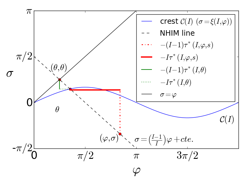
From a geometrical point of view, to find an intersection between a NHIM line and a crest, one throws from a point (θ,θ)(\theta,\theta) on the plane (φ,σ)(\varphi,\sigma) a straight line with slope (I−1)/I(I-1)/I, until it touches the crest 𝒞⁡(I)\mathcal{C}(I). The function τ∗​(I,θ)\tau^{*}(I,\theta) is the time spent to go from a point (θ,θ)(\theta,\theta) in the diagonal σ=φ\sigma=\varphi up to 𝒞⁡(I)\mathcal{C}(I) with a velocity vector 𝐯=−(I,I−1)\mathbf{v}=-(I,I-1), see Fig. 3.

Refer to caption
Fig. 3: Finding τ∗​(I,θ)\tau^{*}(I,\theta) using the straight line σ=φ\sigma=\varphi.

One has to decide the direction for τ∗\tau^{*} using the idea explained above. For example, if we are on a point on the straight line σ=φ\sigma=\varphi, we have to decide if we go up or go down along the NHIM line, i.e., to look for a negative or a positive τ∗​(I,θ)\tau^{*}(I,\theta) (to look at the past or the future). In both cases we are going to detect an intersection with the desired crest, but, in general, different choices give rise to different scattering maps, because we are looking for different homoclinic invariant manifolds Γ\Gamma.

To show another difference between scattering maps from the choice of τ∗\tau^{*} we begin by introducing each kind of scattering map. The first one is inspired in [DH11] and [DS17] for |μ|<0.97\left|\mu\right|<0.97. In these cited cases all scattering maps studied were associated to one of the horizontal crests like in (27). In the same way, we can separate completely the scattering maps associated to the horizontal crests and the scattering maps associated to the vertical crests. Notice that the scattering maps associated to horizontal crests are defined only for values of II satisfying |α⁡(I)|<1/|μ|\left|\alpha(I)\right|<1/\left|\mu\right| whereas the scattering maps associated to the vertical crests are defined only for values of II satisfying |α⁡(I)|>1/|μ|\left|\alpha(I)\right|>1/\left|\mu\right|.

As noted previously, crests are vertical in a neighborhood of I=1I=1 for any value of μ\mu. Therefore, there is no scattering map associated to a horizontal crest close to I=1I=1. Analogously, since |α⁡(0)|=0\left|\alpha(0)\right|=0, crests are horizontal in a neighborhood of I=0I=0 for any value of μ\mu and, therefore, there is no scattering map associated to a vertical crest close to I=0I=0. This implies that these “horizontal” or “vertical” scattering maps are just locally defined, in other words, they are not defined on the whole plane (θ,I)(\theta,I). This motivates to define global scattering maps. Global scattering maps are important because they describe the outer dynamics for large intervals of II and are defined as follows

Definition 17.

A scattering map 𝒮⁡(I,θ)\mathcal{S}(I,\theta) is called a global scattering map if it is defined on all θ∈𝕋\theta\in\mathbb{T} for any fixed II.

Note that 𝒮⁡(I,θ)\mathcal{S}(I,\theta) is a global scattering map as long as τ∗​(I,θ)\tau^{*}(I,\theta) is a global function, i.e., defined on all θ∈𝕋\theta\in\mathbb{T} for any fixed II. If τ∗​(I,θ)\tau^{*}(I,\theta) is smoothly defined, the same will happen to 𝒮⁡(I,θ)\mathcal{S}(I,\theta). Tangencies between NHIM  lines and crests, as well as discontinuities in their intersections give rise to non-smooth scattering maps.

Remark 18.

For instance, in the paper [DS17] devoted to the Hamiltonian (6), it was proven that for 0<μ=a1/a2<0.6250<\mu=a_{1}/a_{2}<0.625, there exist two different global scattering maps. Let us add that for 0.625≤μ<0.970.625\leq\mu<0.97, due to the existence of tangencies between the NHIM lines and the crests, there appear two or six scattering maps. Such multiple scattering maps are indeed piecewise smooth global scattering maps, see Figs. 9–11 of [DS17]. Their discontinuities lie along the tangency locus and were avoided there to construct diffusion paths, just for the sake of simplicity.

For Hamiltonian (7), to extend scattering maps which are in principle only locally defined we have now two options: to combine a scattering map associated to a horizontal crest with a scattering map associated to a vertical crest or to extend the previously called “horizontal” or “vertical” scattering maps. Although the first option may provide a global scattering map, they may appear complex discontinuity sets which give rise to a complicated phase space.

The second option is to apply the same idea used in [DS17] when we defined the scattering map “with holes”. When |α⁡(I)|>1/|μ|\left|\alpha(I)\right|>1/\left|\mu\right|, the horizontal crests are no longer defined for all φ∈𝕋\varphi\in\mathbb{T}, indeed, they become vertical crests defined for all σ∈𝕋\sigma\in\mathbb{T}. Nevertheless, the vertical crests are formed by pieces of horizontal crests. This implies that even for these values of II we can use ξ\xi given in (27) to parameterize some intersections between R⁡(I,φ,σ)R(I,\varphi,\sigma) and 𝒞⁡(I)\mathcal{C}(I). As we can see in Fig. 4, the vertical and horizontal crest 𝒞M\mathcal{C}_{\text{M}} are very close in a neighbourhood of φ=0\varphi=0. When we have a bifurcation from horizontal to vertical crests (or vice versa), it is natural just to change the parameterization from ξM\xi_{\text{M}} to ηM\eta_{\text{M}} for these values of φ\varphi. With this choice the orbits of the scattering map are continuous for θ\theta close to 00 or 2​π2\pi. The same happens with ξm\xi_{\text{m}} and ηm\eta_{\text{m}} for values of φ\varphi close to π\pi. Scattering maps associated to horizontal crests for values of II satisfying |μ​α​(I)|<1\left|\mu\alpha(I)\right|<1 are defined for all φ∈𝕋\varphi\in\mathbb{T}. The extension of them to values of II for φ∈𝕋\varphi\in\mathbb{T} such that |μ​α​(I)​sin⁡φ|<1\left|\mu\alpha(I)\sin\varphi\right|<1 are called extended scattering maps.

Definition 19.

A scattering map 𝒮⁡(I,θ)\mathcal{S}(I,\theta) is called an extended scattering map if it is associated to horizontal crests for which |μ​α​(I)|<1\left|\mu\alpha(I)\right|<1, and is continuously extended to the pieces of the vertical crests where they behave as horizontal crests, that is, for the values φ\varphi such that |μ​α​(I)​sin⁡φ|<1\left|\mu\alpha(I)\sin\varphi\right|<1.

Since we have already seen in Proposition 14 that there exist tangencies between NHIM lines and crests for any value of μ\mu, there are no global scattering maps for Hamiltonian (7). However, there exist extended scattering maps with a domain large enough to provide diffusion paths.

Refer to caption
(a) A piece of ξM​(I,φ)\xi_{\text{M}}(I,\varphi) for I=0.68I=0.68.
Refer to caption
(b) A piece of ηM​(I,σ)\eta_{\text{M}}(I,\sigma) for I=0.72I=0.72.
Fig. 4: Comparison between ξM​(I,φ)\xi_{\text{M}}(I,\varphi) and ηM​(I,σ)\eta_{\text{M}}(I,\sigma) for μ=0.5\mu=0.5, I=0.68I=0.68 and I=0.72I=0.72 respectively.

To illustrate the current scenario we will display the level curves of the reduced Poincaré function ℒ∗​(I,θ)\mathcal{L}^{*}(I,\theta) defined in (19), which up to 𝒪⁡(ε2)\mathcal{O}(\varepsilon^{2}) contain orbits of the scattering map 𝒮⁡(I,θ)\mathcal{S}(I,\theta). We begin by considering μ=0.6\mu=0.6 and the horizontal crest 𝒞M​(I)\mathcal{C}_{\text{M}}(I). In Fig. 5(a) we display the scattering map built using τ∗\tau^{*} defined by the first intersection between RI​(φ,σ)R_{I}(\varphi,\sigma) and 𝒞M​(I)\mathcal{C}_{\text{M}}(I) from σ=φ\sigma=\varphi going down along RI​(φ,σ)R_{I}(\varphi,\sigma). In Fig.5(b), we use a similar idea, but now, form σ=φ\sigma=\varphi going up along RI​(φ,σ)R_{I}(\varphi,\sigma). Alternatively, if we choose τ∗\tau^{*} with minimal absolute value, independently of going up or down, we obtain the scattering map plotted on Fig. 5(c). In this last case, there are orbits of the scattering maps that are not smooth in θ=π\theta=\pi. This happens because we change the homoclinic manifold Γ\Gamma, so we are using, indeed, two different scattering maps. In [DS17] we chose scattering maps associated to a function τ∗\tau^{*} with the minimal absolute value, which were called primary scattering maps. This example show us that is not enough to say what crest is associated to a scattering map, but it is also necessary to make explicit the criterion used for τ∗\tau^{*} (going up or down along the NHIM lines, or choosing a minimal OPEN|τ∗|)\left|\tau^{*}\right|).

Refer to caption
(a) Going down along the NHIM lines RI​(φ,σ)R_{I}(\varphi,\sigma).
Refer to caption
(b) Going up along the NHIM lines RI​(φ,σ)R_{I}(\varphi,\sigma).
Refer to caption
(c) Minimal absolute value of τ∗\tau^{*}.
Fig. 5: Different phase space of scattering maps 𝒮⁡(I,θ)\mathcal{S}(I,\theta) associated to the same horizontal crest CM​(I)C_{\text{M}}(I), for μ=0.6\mu=0.6 and ε=0.01\varepsilon=0.01. The orbits of scattering maps are represented by the blue lines which are, up to 𝒪⁡(ε2)\mathcal{O}(\varepsilon^{2}), level sets of the reduced Poincaré function ℒ∗​(I,θ)\mathcal{L}^{*}(I,\theta). In the red zones the values of II on such orbits decrease, in the green one the values of II increase. The white regions are regions where |μ​α​(I)​sin⁡φ|>1\left|\mu\alpha(I)\sin\varphi\right|>1 is satisfied.

The next lemma is a good example about the criteria for τ∗​(I,θ)\tau^{*}(I,\theta) and its consequences, and is used to prove Proposition 22. Before, a new notation is introduced. An even subindex kk is assigned to the branches 𝒞k​(I)\mathcal{C}_{k}(I) of 𝒞M​(I)\mathcal{C}_{\text{M}}(I) when considering σ,φ∈ℝ\sigma,\,\varphi\in\mathbb{R}

ξk​(I,φ)=−arcsin⁡(α⁡(I)​μ​sin⁡φ)+k​π and ηk=−arcsin⁡(sin⁡σα⁡(I)​μ)+k​π\xi_{k}(I,\varphi)=-\arcsin\left(\alpha(I)\mu\sin\varphi\right)+k\pi\quad\text{ and }\quad\eta_{k}=-\arcsin\left(\frac{\sin\sigma}{\alpha(I)\mu}\right)+k\pi

and an odd subindex kk to the branches 𝒞k​(I)\mathcal{C}_{k}(I) of 𝒞m​(I)\mathcal{C}_{\text{m}}(I) when considering σ,φ∈ℝ\sigma,\,\varphi\in\mathbb{R}

ξk​(I,φ)=arcsin⁡(α⁡(I)​μ​sin⁡φ)+k​π and ηk=arcsin⁡(sin⁡σα⁡(I)​μ)+k​π.\xi_{k}(I,\varphi)=\arcsin\left(\alpha(I)\mu\sin\varphi\right)+k\pi\quad\text{ and }\quad\eta_{k}=\arcsin\left(\frac{\sin\sigma}{\alpha(I)\mu}\right)+k\pi.

We notice that the crests 𝒞⁡(I)\mathcal{C}(I) are naturally defined for (φ,σ)∈𝕋2(\varphi,\sigma)\in\mathbb{T}^{2} and give rise to two different crests 𝒞M​(I)\mathcal{C}_{\text{M}}(I), 𝒞m​(I)\mathcal{C}_{\text{m}}(I) (except for the singular case |μ​α​(I)|=1\left|\mu\alpha(I)\right|=1). When we run now over real values of φ,σ\varphi,\,\sigma, we may have an infinite number of crests 𝒞k​(I)\mathcal{C}_{k}(I), where even (odd) values of kk are assigned to the branches of 𝒞M​(I)\mathcal{C}_{\text{M}}(I) (𝒞m​(I)\mathcal{C}_{\text{m}}(I)). Among them, we are going to use 𝒞0​(I)\mathcal{C}_{0}(I), 𝒞1​(I)\mathcal{C}_{1}(I) and 𝒞2​(I)\mathcal{C}_{2}(I).

Lemma 20.

Let ℒ0∗\mathcal{L}_{\text{0}}^{*} and ℒ2∗\mathcal{L}_{\text{2}}^{*} be reduced Poincaré functions associated to the same crest 𝒞⁡(I)\mathcal{C}(I), where for ℒ0∗\mathcal{L}_{\text{0}}^{*} we look at the first intersection points “under” σ=φ\sigma=\varphi, that is, with 𝒞0​(I)\mathcal{C}_{0}(I), and for ℒ2∗\mathcal{L}_{\text{2}}^{*} we look at the first intersection points “over” σ=φ\sigma=\varphi, that is, with 𝒞2​(I)\mathcal{C}_{2}(I). Then we have

∂ℒ0∗∂θ​(I,θ)=−∂ℒ2∗∂θ​(I,2​π−θ).\frac{\partial\mathcal{L}_{\text{0}}^{*}}{\partial\theta}\left(I,\theta\right)=-\frac{\partial\mathcal{L}_{\text{2}}^{*}}{\partial\theta}\left(I,2\pi-\theta\right). (30)
Remark 21.

We say “under" σ=φ\sigma=\varphi and “over" σ=φ\sigma=\varphi for intersection points going down or up along RI​(φ,σ)R_{I}(\varphi,\sigma), respectively on (φ,ξ0​(I,φ))(\varphi,\xi_{0}(I,\varphi)) and (φ,ξ2​(I,φ))(\varphi,\xi_{2}(I,\varphi)), because when the horizontal crest 𝒞M​(I)\mathcal{C}_{\text{M}}(I) is defined for all φ∈𝕋\varphi\in\mathbb{T} the graphs (φ,ξ0​(I,φ))(\varphi,\xi_{0}(I,\varphi)) of 𝒞0​(I)\mathcal{C}_{0}(I) and (φ,ξ2​(I,φ))(\varphi,\xi_{2}(I,\varphi)) of 𝒞2​(I)\mathcal{C}_{2}(I) are under and over the straight line σ=φ\sigma=\varphi.

Proof.

Let ℒ∗\mathcal{L}^{*} be a reduced Poincaré function (19)-(17), then

∂ℒ∗∂θ​(I,θ)=A1​(I)​sin⁡(θ−I​τ∗​(I,θ))I−1.\frac{\partial\mathcal{L}^{*}}{\partial\theta}\left(I,\theta\right)=\frac{A_{1}(I)\sin(\theta-I\tau^{*}(I,\theta))}{I-1}.

So, equation (30) is satisfied if, and only if

sin⁡(θ−I​τ0∗​(I,θ))=sin⁡(θ−I⁡(−τ2∗​(I,2​π−θ))).\sin(\theta-I\tau_{\text{0}}^{*}(I,\theta))=\sin(\theta-I(-\tau_{\text{2}}^{*}(I,2\pi-\theta))). (31)

We assume that the crest is horizontal and given by the graph of ξM\xi_{\text{M}}, the other cases are analogous. Indeed, we are going to use

ξ0​(I,φ)=−arcsin⁡(μ​α​(I)​sin⁡φ) and ξ2​(I,φ)=ξ0​(I,φ)+2​π.\xi_{\text{0}}(I,\varphi)=-\arcsin(\mu\alpha(I)\sin\varphi)\quad\text{ and }\quad\xi_{\text{2}}(I,\varphi)=\xi_{\text{0}}(I,\varphi)+2\pi. (32)

This implies that the intersection point “under” σ=φ\sigma=\varphi is a point on the curve parameterized by ξ0​(I,φ)\xi_{\text{0}}(I,\varphi). Otherwise, the intersection “over” σ=φ\sigma=\varphi is a point on the curve parameterized by ξ2​(I,φ)\xi_{\text{2}}(I,\varphi). As the slope of the NHIM lines is (I−1)/I(I-1)/I, given a point (θ,θ)(\theta,\theta), we obtain

ξ2​(I,θ−I​τ2∗​(I,θ))−θθ−I​τ2∗​(I,θ)−θ=I−1I,\frac{\xi_{\text{2}}(I,\theta-I\tau_{\text{2}}^{*}(I,\theta))-\theta}{\theta-I\tau_{\text{2}}^{*}(I,\theta)-\theta}=\frac{I-1}{I},

which can be rewritten as

2​π+ξ0​(I,θ−I​τ2∗​(I,θ))−θ−I​τ2∗​(I,θ)=I−1I.\frac{2\pi+\xi_{\text{0}}(I,\theta-I\tau_{\text{2}}^{*}(I,\theta))-\theta}{-I\tau_{\text{2}}^{*}(I,\theta)}=\frac{I-1}{I}.

From this equation, we obtain an expression for τ2∗​(I,θCLOSE\tau_{\text{2}}^{*}(I,\theta)

τ2∗​(I,θ)=−(2​π+ξ0​(I,θ−I​τ2∗​(I,θ))−θ)I−1.\tau_{\text{2}}^{*}(I,\theta)=\frac{-\left(2\pi+\xi_{\text{0}}(I,\theta-I\tau_{\text{2}}^{*}(I,\theta))-\theta\right)}{I-1}.

From the expressions of τ2∗​(I,θ)\tau_{\text{2}}^{*}(I,\theta) above and (32),

τ2∗​(I,2​π−θ)=(ξ0​(I,θ−I⁡(−τ2∗​(I,2​π−θ)))+θ)I−1,\tau_{\text{2}}^{*}(I,2\pi-\theta)=\frac{\left(\xi_{\text{0}}(I,\theta-I\left(-\tau_{\text{2}}^{*}(I,2\pi-\theta)\right))+\theta\right)}{I-1},

and therefore

θ−(I−1)​(−τ2∗​(I,2​π−θ))=ξ0​(I,θ−(I−1)​(−τ2∗​(I,2​π−θ))),\theta-(I-1)(-\tau_{\text{2}}^{*}(I,2\pi-\theta))=\xi_{\text{0}}(I,\theta-(I-1)(-\tau_{\text{2}}^{*}(I,2\pi-\theta))),

which implies that −τ2∗​(I,2​π−θ)-\tau_{\text{2}}^{*}(I,2\pi-\theta) is a time of intersection between the NHIM line and the curve parameterized by ξ0\xi_{\text{0}}. In the case that there exists only one intersection point, this implies

τ0∗​(I,θ)=τ2∗​(I,2​π−θ).\tau_{\text{0}}^{*}(I,\theta)=\tau_{\text{2}}^{*}(I,2\pi-\theta).

So, condition (31) is satisfied. ∎

Proposition 22.

Let 𝒮1​(I,θ)\mathcal{S}_{\text{1}}(I,\theta) be the scattering map associated to the graphs of ξ1\xi_{\text{1}} and η1\eta_{\text{1}} of 𝒞1​(I)\mathcal{C}_{1}(I). Assuming a1,a2>0a_{1},a_{2}>0, for any II there exists a θ+\theta_{+} such that I˙>0\dot{I}>0 for θ∈(π,θ+)\theta\in(\pi,\theta_{+}). Moreover, θ+≥3​π/2\theta_{+}\geq 3\pi/2 for I∉(−1/2,1/2)I\notin(-1/2,1/2).

Proof.

A proof is given in Appendix A. ∎

Remark 23.

If a1<0a_{1}<0, we have that there exists a θ−\theta_{-} such that I˙>0\dot{I}>0 for any θ∈(θ−,π)\theta\in(\theta_{-},\pi).

Remark 24.

An analogous proposition holds for 𝒮2​(I,θ)\mathcal{S}_{\text{2}}(I,\theta), the scattering map associated to the graphs of ξ2\xi_{\text{2}} and η2\eta_{\text{2}} of 𝒞2​(I)\mathcal{C}_{2}(I). In such case, there is a θ+\theta_{+} such that I˙≥0\dot{I}\geq 0 for any θ∈(θ+,2​π)\theta\in(\theta_{+},2\pi) where θ≥3​π/2\theta\geq 3\pi/2 for I∈(1/2,3/2)I\in(1/2,3/2).

Note that this proposition leads us to ensure the diffusion in an analogous way to the one used to prove Theorem 4 in [DS17]. Next, the diffusion mechanism is stated and the Arnold diffusion is proven.

4 Arnold Diffusion

In this section we are going to complete our goal proving the existence of global instability or Arnold diffusion, that is, Theorem 1.

We begin by presenting some general geometrical properties of the scattering maps that we have to take into account to prove the theorem of diffusion. The first one reduces the study of scattering maps to positive values of μ\mu. More precisely, we have the lemma below

Lemma 25.

The scattering map for a value of μ\mu and s=πs=\pi, associated to the intersection between R⁡(I,φ,s)R(I,\varphi,s) and Cm​(I)C_{\text{m}}(I) (CM​(I)C_{\text{M}}(I)) has the same geometrical properties as the scattering map for −μ-\mu and s=0s=0, associated to the intersection between Rθ​(I)R_{\theta}(I) and CM​(I)C_{\text{M}}(I) (Cm​(I)C_{\text{m}}(I)), i.e.,

Sm​(M)μ​(I,φ,π)=SM​(m)−μ​(I,φ,0)=𝒮M​(m)−μ​(I,θ)S^{\mu}_{\text{m}(\text{M})}(I,\varphi,\pi)=S^{-\mu}_{\text{M}(\text{m})}(I,\varphi,0)=\mathcal{S}^{-\mu}_{\text{M}(\text{m})}(I,\theta)
Proof.

First, we look for τm∗\tau^{*}_{\text{m}} such that the NHIM segment R⁡(I,φ,s)R(I,\varphi,s) intersects the crest Cm​(I)C_{\text{m}}(I). If we fix s=πs=\pi, we have from (17) and (18):

Lμ,m∗​(I,φ,π)=A1​(I)​cos⁡(φ−I​τm∗​(I,φ,π))+A2​(I)​cos⁡(φ−π−(I−1)​τm∗​(I,φ,π)).L_{\mu,\text{m}}^{*}(I,\varphi,\pi)=A_{1}(I)\cos(\varphi-I\tau_{\text{m}}^{*}(I,\varphi,\pi))+A_{2}(I)\cos(\varphi-\pi-(I-1)\tau_{\text{m}}^{*}(I,\varphi,\pi)). (33)

Besides, τ∗\tau^{*} satisfies

μ​α​(I)​sin⁡(φ−I​τm∗)+sin⁡(φ−π−(I−1)​τm∗)=0,\mu\alpha(I)\sin(\varphi-I\tau_{\text{m}}^{*})+\sin(\varphi-\pi-(I-1)\tau_{\text{m}}^{*})=0,

or

−μ​α​(I)​sin⁡(φ−I​τm∗)+sin⁡(φ−(I−1)​τm∗)=0.-\mu\alpha(I)\sin(\varphi-I\tau_{\text{m}}^{*})+\sin(\varphi-(I-1)\tau_{\text{m}}^{*})=0.

We have that φ−π−(I−1)​τm∗(mod2​π)=ξm​(I,φ−I​τm∗)\varphi-\pi-(I-1)\tau_{\text{m}}^{*}\pmod{2\pi}=\xi_{\text{m}}(I,\varphi-I\tau_{\text{m}}^{*}) with π/2≤ξm≤3​π/2\pi/2\leq\xi_{\text{m}}\leq 3\pi/2. Then, for each τm∗\tau^{*}_{\text{m}} there exists a K∈ℤK\in\mathbb{Z} such that

π2<φ−π−(I−1)​τm∗+2​π​K<3​π2.\frac{\pi}{2}<\varphi-\pi-(I-1)\tau^{*}_{\text{m}}+2\pi K<\frac{3\pi}{2}.

This implies

3​π2<φ−(I−1)​τm∗+2​π​K and φ−(I−1)​τm∗+2​π​(K−1)<π2.\frac{3\pi}{2}<\varphi-(I-1)\tau^{*}_{\text{m}}+2\pi K\quad\text{ and }\quad\varphi-(I-1)\tau^{*}_{\text{m}}+2\pi(K-1)<\frac{\pi}{2}.

Therefore,

φ−(I−1)​τm∗(mod2​π)<π2 or φ−(I−1)​τm∗(mod2​π)>3​π2.\varphi-(I-1)\tau^{*}_{m}\pmod{2\pi}<\frac{\pi}{2}\quad\text{ or }\quad\varphi-(I-1)\tau^{*}_{m}\pmod{2\pi}>\frac{3\pi}{2}.

We can conclude that φ−(I−1)​τm∗(mod2​π)=ξM​(I,φ−I​τm∗)\varphi-(I-1)\tau^{*}_{m}\pmod{2\pi}=\xi_{\text{M}}(I,\varphi-I\tau^{*}_{\text{m}}). Therefore τm∗​(I,φ,π)\tau_{\text{m}}^{*}(I,\varphi,\pi) for μ\mu is equal to τM∗​(I,φ,0)\tau_{\text{M}}^{*}(I,\varphi,0) for −μ-\mu. From (33), Lμ,m∗​(I,φ,π)L^{*}_{\mu,\text{m}}(I,\varphi,\pi) satisfies

Lμ,m∗​(I,φ,π)\displaystyle L_{\mu,\text{m}}^{*}(I,\varphi,\pi) =\displaystyle= A1​(I)​cos⁡(φ−τM∗​(I,φ,0))+(−A2​(I))​cos⁡(φ−(I−1)​τM∗​(I,φ,0))\displaystyle A_{1}(I)\cos(\varphi-\tau_{\text{M}}^{*}(I,\varphi,0))+(-A_{2}(I))\cos(\varphi-(I-1)\tau_{\text{M}}^{*}(I,\varphi,0))
=\displaystyle= L−μ,M∗​(I,φ,0).\displaystyle L_{-\mu,\text{M}}^{*}(I,\varphi,0).

Since Lμ,m∗​(⋅,⋅,π)L^{*}_{\mu,\text{m}}(\cdot,\cdot,\pi) and L−μ,M∗​(⋅,⋅,0)L^{*}_{-\mu,\text{M}}(\cdot,\cdot,0) coincide, their derivatives too and this implies that

Smμ​(I,φ,π)=SM−μ​(I,φ,0)=𝒮M−μ​(I,θ).S^{\mu}_{\text{m}}(I,\varphi,\pi)=S^{-\mu}_{\text{M}}(I,\varphi,0)=\mathcal{S}^{-\mu}_{\text{M}}(I,\theta).

∎

From now on, just to simplify the exposition, a1a_{1} and a2a_{2} are considered positive. The same strategy used in [DS17] is applied to prove the existence the diffusion: we combine the scattering map in an interval of θ\theta where I˙>0\dot{I}>0 and the inner map to build a diffusion pseudo-orbit. Then we apply shadowing results to get the existence of a diffusion orbit.

Since I=0I=0 and I=1I=1 are resonance values, the application of the inner map must be more careful, because in these resonance regions, for some orbits, the value of II decreases in order 𝒪⁡(ε)\mathcal{O}(\sqrt{\varepsilon}), i. e., the tori cannot be considered flat. We study the transversality between the foliations of invariant sets of the inner and the scattering map in resonant and non-resonant regions and its image under the scattering map 𝒮\mathcal{S}. For more details and a more general case, the reader is referred to [DH09].

Consider the resonant region associated to I=0I=0. In such region, the tori can be approximated by F0​(I,φ)F^{0}(I,\varphi) given in (15). The tranversality between invariant sets of the inner and the scattering map holds if the gradient vectors of the level curves of F0F^{0} and ℒ∗\mathcal{L}^{*} are not parallel vectors, or equivalently,

{F0​(I,θ),ℒ∗​(I,θ)}≠0,\left\{F^{0}(I,\theta),\mathcal{L}^{*}(I,\theta)\right\}\neq 0,

where {,}\left\{,\right\} is the Poisson bracket,

{F0,ℒ∗}=∂F0∂θ​∂ℒ∂I−∂F0∂I​∂ℒ∂θ.\left\{F^{0},\mathcal{L^{*}}\right\}=\frac{\partial F^{0}}{\partial\theta}\frac{\partial\mathcal{L}}{\partial I}-\frac{\partial F^{0}}{\partial I}\frac{\partial\mathcal{L}}{\partial\theta}.

From (15), the partial derivatives of F0F^{0} are

∂F0∂I=I\displaystyle\frac{\partial F^{0}}{\partial I}=I and ∂F0∂θ=−ε​a1​sin⁡θ,\displaystyle\frac{\partial F^{0}}{\partial\theta}=-\varepsilon a_{1}\sin\theta,

and since ℒ∗​(I,θ)=A1​(I)​cos⁡(θ−I​τ∗​(I,θ))+A2​(I)​cos⁡(θ−(I−1)​τ∗​(I,θ))\mathcal{L}^{*}(I,\theta)=A_{1}(I)\cos(\theta-I\tau^{*}(I,\theta))+A_{2}(I)\cos(\theta-(I-1)\tau^{*}(I,\theta)), we have the partial derivatives given by

∂ℒ∗∂θ=A1​(I)​sin⁡(θ−I​τ∗)I−1,\frac{\partial\mathcal{L}^{*}}{\partial\theta}=\frac{A_{1}(I)\sin(\theta-I\tau^{*})}{I-1},
∂ℒ∗∂I=A1′​(I)​cos⁡(θ−I​τ∗)+A2′​(I)​cos⁡(θ−(I−1)​τ∗)+A1​(I)​τ∗​sin⁡(θ−I​τ∗)+A2​(I)​τ∗​sin⁡(θ−(I−1)​τ∗).\frac{\partial\mathcal{L}^{*}}{\partial I}=A_{1}^{\prime}(I)\cos(\theta-I\tau^{*})+A_{2}^{\prime}(I)\cos(\theta-(I-1)\tau^{*})+A_{1}(I)\tau^{*}\sin(\theta-I\tau^{*})+A_{2}(I)\tau^{*}\sin(\theta-(I-1)\tau^{*}).

Note that if |I|>𝒪⁡(ε)\left|I\right|>\mathcal{O}(\varepsilon), ∂F0/∂I\partial F^{0}/\partial I dominates ∂F0/∂θ\partial F^{0}/\partial\theta, so the Poisson bracket above can be reduced to

{F0,ℒ∗}≃−∂F0∂I​∂ℒ∂θ=−I​A1​(I)​sin⁡(θ−I​τ∗)I−1\left\{F^{0},\mathcal{L^{*}}\right\}\simeq-\frac{\partial F^{0}}{\partial I}\frac{\partial\mathcal{L}}{\partial\theta}=\frac{-IA_{1}(I)\sin(\theta-I\tau^{*})}{I-1}

Expanding sin⁡(θ−I​τ∗)\sin(\theta-I\tau^{*}) in Taylor’s series around I=0I=0, we have

sin⁡(θ−I​τ∗)=sin⁡θ+𝒪⁡(I),\sin(\theta-I\tau^{*})=\sin\theta+\mathcal{O}(I),

which implies {F0,ℒ∗}=0\left\{F^{0},\mathcal{L}^{*}\right\}=0 if, and only if, θ≈0,π\theta\approx 0,\pi, assuming that 𝒪⁡(I)\mathcal{O}(I) is small enough.

Now, we consider I=𝒪⁡(ε)I=\mathcal{O}(\varepsilon) and look at the intersections between the NHIM lines and the graph of ξ1\xi_{1}. Note that as the value of II is close to 00 we can assume that the crests are horizontal. Using Taylor’s series we can write

sin⁡(θ−I​τ∗)=sin⁡θ+𝒪⁡(I)\displaystyle\sin(\theta-I\tau^{*})=\sin\theta+\mathcal{O}(I) cos⁡(θ−I​τ∗)=cos⁡θ+𝒪⁡(I)\displaystyle\cos(\theta-I\tau^{*})=\cos\theta+\mathcal{O}(I)
sin⁡(θ−(I−1)​τ∗)=𝒪⁡(I)\displaystyle\sin(\theta-(I-1)\tau^{*})=\mathcal{O}(I) cos⁡(θ−(I−1)​τ∗)=−1+𝒪⁡(I).\displaystyle\cos(\theta-(I-1)\tau^{*})=-1+\mathcal{O}(I).

This implies

{F0,ℒ∗}=−I​A1​(I)​sin⁡θI−1−ε​a1​sin⁡θ⁡(A1′​(I)​cos⁡θ−A2′​(I)+A1​(I)​τ∗​sin⁡θ)+𝒪⁡(I2,ε​I).\left\{F^{0},\mathcal{L}^{*}\right\}=-\frac{IA_{1}(I)\sin\theta}{I-1}-\varepsilon a_{1}\sin\theta\left(A_{1}^{\prime}(I)\cos\theta-A_{2}^{\prime}(I)+A_{1}(I)\tau^{*}\sin\theta\right)+\mathcal{O}(I^{2},\varepsilon I). (34)

Taylor expanding the functions A1​(I)A_{1}(I), A1′​(I)A_{1}^{\prime}(I) and A2′​(I)A_{2}^{\prime}(I) around I=0I=0, we obtain

A1(I)=4a1+𝒪(I)2,A1′(I)=𝒪(I) and A2′(I)=a2π(πcothπ/2−2)csch(π/2)+𝒪(I)A_{1}(I)=4a_{1}+\mathcal{O}(I{{}^{2}}),\quad A_{1}^{\prime}(I)=\mathcal{O}(I)\text{ and }A_{2}^{\prime}(I)=a_{2}\pi(\pi\coth\pi/2-2)\text{csch}(\pi/2)+\mathcal{O}(I)

Plugging these expressions in (34), we set

{F0,ℒ∗}=−4​a1​I​sin⁡θI−1−ε​a1​sin⁡θ⁡[a2​π​(π​coth⁡π/2−2)​csch​(π/2)+4​a1​(π−θ)​sin⁡θ]+𝒪⁡(I2,I​ε).\left\{F^{0},\mathcal{L^{*}}\right\}=-\frac{4a_{1}I\sin\theta}{I-1}-\varepsilon a_{1}\sin\theta\left[a_{2}\pi(\pi\coth\pi/2-2)\text{csch}(\pi/2)+4a_{1}(\pi-\theta)\sin\theta\right]+\mathcal{O}(I^{2},I\varepsilon).

So, {F0,ℒ∗}=0⇔a1​sin⁡θ⁡[−4​II−1−ε​a2​π​(π​coth⁡π/2−2)​csch​(π/2)+ε​4​(π−θ)​sin⁡θ]=0\left\{F^{0},\mathcal{L^{*}}\right\}=0\Leftrightarrow a_{1}\sin\theta\left[\frac{-4I}{I-1}-\varepsilon a_{2}\pi(\pi\coth\pi/2-2)\text{csch}(\pi/2)+\varepsilon 4(\pi-\theta)\sin\theta\right]=0. In other words, we do not have transversality if, and only if, θ=0,π\theta=0,\pi or satisfies

(π−θ)​sin⁡θ=Iε​a1+OPENπ⁡(coth⁡π/2−2)​csch​π/2)4,(\pi-\theta)\sin\theta=\frac{I}{\varepsilon a_{1}}+\frac{\pi(\coth\pi/2-2)\text{csch}\pi/2)}{4},

which is not an horizontal curve in the plane (θ,I)(\theta,I) and is transversal to an invariant torus of the inner dynamics.

For the other resonant region I=1I=1, F1F^{1} is very similar. Assuming I−1=𝒪⁡(ε)I-1=\mathcal{O}(\varepsilon), we have

{F1,ℒ∗}=a2​sin⁡θ⁡{4​(I−1I)−ε⁡[π​a1​(2−π​coth⁡(π/2))​csch​(π/2)+4​a2​sin⁡θ]}.\left\{F^{1},\mathcal{L}^{*}\right\}=a_{2}\sin\theta\left\{4\left(\frac{I-1}{I}\right)-\varepsilon\left[\pi a_{1}(2-\pi\coth(\pi/2))\text{csch}(\pi/2)+4a_{2}\sin\theta\right]\right\}.

Applying the same methodology, we obtain an analogous result for the other resonant region F1F^{1}. In short, we conclude that the image 𝒮⁡(𝒯i)\mathcal{S}(\mathcal{T}_{i}) of an invariant torus 𝒯i\mathcal{T}_{i} of the inner map under the scattering map intersects tranversally another invariant torus 𝒯i+1\mathcal{T}_{i+1} of the inner map.

Finally, in the non-resonant region, we notice that

{Fnr,ℒ∗}=−∂Fnr∂I​∂ℒ∗∂θ=−I​A1​(I)​sin⁡(θ−I​τ∗)I−1,\left\{F^{\text{nr}},\mathcal{L}^{*}\right\}=-\frac{\partial F^{\text{nr}}}{\partial I}\frac{\partial\mathcal{L}^{*}}{\partial\theta}=-\frac{IA_{1}(I)\sin(\theta-I\tau^{*})}{I-1},

just the same expression as the one for the resonance I=0I=0, so the transversality between invariant sets of the inner and the scattering map follows.

Now, a constructive proof of Theorem 1 is presented. This proof is similar to the proof presented in [DS17], but now, there is no any piece of “highway” or fast vertical lines where |I|\left|I\right| is large. So, the inner map is applied more times.

4.1 Proof of Theorem 1

Proof.

First of all we have to choose what scattering map we use. This choice depends on the sign of μ\mu as explained in Lemma 25. Assuming μ>0\mu>0, we take 𝒮1​(I,θ)\mathcal{S}_{\text{1}}(I,\theta), the global scattering map associated to the graphs of ξ1\xi_{\text{1}} and η1\eta_{\text{1}}. If a1>0a_{1}>0, by Proposition 22 for any II there exists an interval θ∈(π,θ+)\theta\in(\pi,\theta_{+}) where I˙>0\dot{I}>0. Define HrH_{\text{r}} the set (ρ,θ+)×[−I∗,I∗]\left(\rho,\theta_{+}\right)\times\left[-I^{*},I^{*}\right], where ρ=π+δ\rho=\pi+\delta is such that π<ρ<θ+\pi<\rho<\theta_{+} and the transversality between NHIM lines and ℒ1∗\mathcal{L}_{1}^{*} holds. We first construct a pseudo-orbit {(Ii,θi):i=0,…,N1}⊂Hr\{(I_{i},\theta_{i}):i=0,\dots,N_{1}\}\subset H_{\text{r}} with I0=−I∗I_{0}=-I^{*} and θN1\theta_{N_{1}} as close as possible to ρ\rho. Note that all these points lie in the same level curve of ℒ1∗\mathcal{L}_{\text{1}}^{*}, that is, ℒ1∗​(I0,θ0)=ℒ1∗​(Ii,θi)\mathcal{L}_{\text{1}}^{*}(I_{0},\theta_{0})=\mathcal{L}_{\text{1}}^{*}(I_{i},\theta_{i}), i=1,…,N1i=1,\dots,N_{1}. Applying the inner dynamics, we get (IN1+1,θN1+1)=ϕtN1​(IN1,θN1)(I_{\text{N}_{1}+1},\theta_{\text{N}_{1}+1})=\phi_{t_{N_{1}}}(I_{\text{N}_{1}},\theta_{\text{N}_{1}}) with θN1+1∈(ρ,θ+)\theta_{\text{N}_{1}+1}\in(\rho,\theta_{+}) and then we construct a pseudo-orbit {(Ii,θi):i=N1+1,…,N1+M1}⊂ℒ1∗(IN1+1,θN1+1)=lN1+1\{(I_{i},\theta_{i}):i=N_{1}+1,\dots,N_{1}+M_{1}\}\subset\mathcal{L}_{\text{1}}^{*}(I_{\text{N}_{1}+1},\theta_{\text{N}_{1}+1})=l_{\text{N}_{1}+1} with θi∈(ρ,θN1+1)\theta_{i}\in(\rho,\theta_{\text{N}_{1}+1}), θ+−θN1+M1=𝒪⁡(ε2)\theta_{+}-\theta_{\text{N}_{1}+\text{M}_{1}}=\mathcal{O}(\varepsilon^{2}). Applying the inner dynamics, we get (IN1+M1+1,θN1+M1+1)=ϕtN1+M1​(IN1+M1,θN1+M1)(I_{\text{N}_{1}+\text{M}_{1}+1},\theta_{\text{N}_{1}+\text{M}_{1}+1})=\phi_{t_{\text{N}_{1}+\text{M}_{1}}}(I_{\text{N}_{1}+\text{M}_{1}},\theta_{\text{N}_{1}+\text{M}_{1}}) with θN1+M1+1∈(ρ,θ+)\theta_{\text{N}_{1}+\text{M}_{1}+1}\in(\rho,\theta_{+}). Recursively, we construct a pseudo-orbit {(Ii,θi):i=N1+1,…,N2}\{(I_{i},\theta_{i}):i=\text{N}_{1}+1,\dots,\text{N}_{2}\} such that IN2≥I∗I_{\text{N}_{2}}\geq I^{*}. In the same ways as in [DS17] (Theorem 4), we can apply shadowing techniques of [FM00, FM03, GLS14], due to the fact that the inner dynamics is simple enough to satisfy the required hypothesis of these references, to prove the existence of a diffusion trajectory. If a10<0a_{10}<0, changing HrH_{\text{r}} to Hl=(θ+,π)H_{\text{l}}=\left(\theta_{+},\pi\right) all the previous reasoning applies. ∎

Remark 26.

Considering Remark 4, Remark 9, Remark 12 and Remark 16, for any r∈(0,1)r\in(0,1), an equivalent diffusion result is readily obtained.

5 Piecewise smooth global scattering maps

In this section, the geometric freedom of the choice of τ∗\tau^{*} is explored. Until now, only two different scattering maps have been used to build a global one, and this was enough to ensure diffusion. But, with this approach, finding a diffusion pseudo-orbit is not always easy enough and this pseudo-orbit can be also complicated. This depends simply on the “aspect" of the scattering map obtained.

We now suggest a new criterion to choose τ∗\tau^{*}: to take the minimal value for |τ∗|\left|\tau^{*}\right| for any (θ,I)(\theta,I). This provides us with a piecewise smooth global scattering map with a good property: the phase space of this scattering map which is 𝒪⁡(ε2)\mathcal{O}(\varepsilon^{2})-close to the level sets of the reduced Poincaré function ℒ∗​(I,θ)\mathcal{L}^{*}(I,\theta) associated to the chosen τ∗\tau^{*} is simpler and “cleaner” than the phase spaces of other scattering maps displayed up to now. By a cleaner scattering map, we mean that we can easily identify and understand the orbits of the scattering maps, except for a small region which contains the tangency locus.

Refer to caption
(a) Piecewise scattering map for μ=0.3\mu=0.3.
Refer to caption
(b) Piecewise scattering map for μ=0.5\mu=0.5.
Refer to caption
(c) Piecewise scattering map for μ=0.9\mu=0.9.
Refer to caption
(d) Piecewise scattering map for μ=1.5\mu=1.5.
Fig. 6: Examples of piecewise smooth global scattering maps. The orbits of scattering maps are represented by the blue lines. In the red zones the values of II on such orbits decrease, in the green one the values of II increase.

Besides, the zones where the value of II is increased or decreased under the scattering map is well behaved. II decreases for θ∈(0,π)\theta\in(0,\pi) (the red region on all pictures in Fig. 6) and II increases for θ∈(π,2​π)\theta\in(\pi,2\pi) (the green region on all pictures in Fig. 6). So it is easy to infer that for finding a diffusion pseudo-orbit it is enough to build a combination between the inner map and this scattering map restricted to (π,2​π)(\pi,2\pi), for example if an increased value of II is wished. The same idea used in the proof of Theorem 1.

Observe that the scattering maps we are now considering are a mix of the scattering maps studied previously. As an example, we illustrate the scattering map obtained for μ=0.9\mu=0.9. Such scattering map can be divided into three regions and in each region, the scattering map coincides with a scattering map studied before.

Refer to caption
Fig. 7: A piecewise smooth global scattering map divided into 3 regions. The vertical black lines are the boundaries of the domains of smooth scattering maps.

In Fig. 7, for regions I (0<θ<π/20<\theta<\pi/2), II (π/2<θ<3​π/2\pi/2<\theta<3\pi/2) and III (3​π/2<θ<2​π3\pi/2<\theta<2\pi) the scattering map has the following correspondence:

  • I

    Extended scattering map 𝒮0​(I,θ)\mathcal{S}_{0}(I,\theta) associated to the horizontal 𝒞M​(I)\mathcal{C}_{\text{M}}(I) “under" σ=φ\sigma=\varphi.

  • II

    Extended scattering map 𝒮1​(I,θ)\mathcal{S}_{1}(I,\theta) associated to the horizontal 𝒞m​(I)\mathcal{C}_{\text{m}}(I).

  • III

    Extended scattering map 𝒮2​(I,θ)\mathcal{S}_{2}(I,\theta) associated to the horizontal 𝒞M​(I)\mathcal{C}_{\text{M}}(I) “over" σ=φ\sigma=\varphi.

If extended scattering maps are not considered and we just use scattering maps associated to horizontal and vertical crests, one can see that these scattering maps can be divided into 6 regions, i.e., they can be viewed as a combination of up to 6 scattering maps.

Another property of these scattering maps is the loss of differentiability on the straight lines θ=π/2\theta=\pi/2 and θ=3​π/2\theta=3\pi/2. The vector field associated to the Hamiltonian −ℒi∗-\mathcal{L}_{i}^{*} defined around these discontinuity lines behaves as the vector fields studied in non-smooth dynamics theory. More precisely, we can find regions with slide and unstable slide behavior [Fil88]. In a future work, we envisage to design special pseudo-orbits along these discontinuity lines using such theory. Note that these pseudo-orbits would be very similar to the “highways" defined in [DS17], so in principle, one can expect fast and simple diffusion along these discontinuity lines.

Acknowledgments

The authors would like to express their gratitude to the anonymous referees for their comments and suggestions which have contributed to improved the final form of this paper. We also thank C. Simó for several discussions and comments.

Appendix A Proof of Proposition 22

Proposition 22.

Let 𝒮1​(I,θ)\mathcal{S}_{\text{1}}(I,\theta) be the scattering map associated to the graphs ξ1\xi_{\text{1}} and η1\eta_{\text{1}}. Assuming a1,a2>0a_{1},a_{2}>0, then for any II, there exists a θ+\theta_{+} such that I˙>0\dot{I}>0 for θ∈(π,θ+)\theta\in(\pi,\theta_{+}). Moreover, θ+≥3​π/2\theta_{+}\geq 3\pi/2 for I∉(−1/2,1/2)I\notin(-1/2,1/2).

Proof.

We have

I˙=∂ℒ∗∂θ​(I,θ)=A1​(I)​sin⁡(θ−I​τ∗​(I,θ))I−1=−A2​(I)​sin⁡(θ−(I−1)​τ∗​(I,θ)CLOSEI.\dot{I}=\frac{\partial\mathcal{L}^{*}}{\partial\theta}(I,\theta)=\frac{A_{1}(I)\sin(\theta-I\tau^{*}(I,\theta))}{I-1}=-\frac{A_{2}(I)\sin(\theta-(I-1)\tau^{*}(I,\theta)}{I}. (35)

where A1​(I)A_{1}(I) and A2​(I)A_{2}(I) are positive, because a1,a2>0a_{1},\,a_{2}>0. Notice that μ=a1/a2>0\mu=a_{1}/a_{2}>0.

Note that as (I,φ=π,θ=π)(I,\varphi=\pi,\theta=\pi) is always on the crest 𝒞m​(I)\mathcal{C}_{\text{m}}(I), τ∗​(I,π)=0\tau^{*}(I,\pi)=0 for all II.

Consider first the case of horizontal crests (|α⁡(I)​μ|<1\left|\alpha(I)\mu\right|<1).

  • a)

    For I<0I<0, the function α⁡(I)\alpha(I) introduced in (26) satisfies α⁡(I)>0\alpha(I)>0, and from (27), sin⁡(ξ1​(I,φ))​sin⁡φ=−μ​α​(I)​sin⁡φ≤0\sin(\xi_{\text{1}}(I,\varphi))\sin\varphi=-\mu\alpha(I)\sin\varphi\leq 0. Take θ=3​π2\theta=\frac{3\pi}{2}; since I<0I<0, the slope m=(I−1)/Im=(I-1)/I of the NHIM lines is greater than 1. Therefore, 3​π/2−I​τ1∗​(I,3​π/2)∈(π,3​π/2)3\pi/2-I\tau_{\text{1}}^{*}(I,3\pi/2)\in(\pi,3\pi/2). This implies that for any θ∈(π,3​π/2)\theta\in(\pi,3\pi/2), θ−I​τ1∗​(I,θ)∈(π,3​π/2)\theta-I\tau_{\text{1}}^{*}(I,\theta)\in(\pi,3\pi/2), so sin⁡(θ−I​τ1∗)<0\sin(\theta-I\tau_{\text{1}}^{*})<0. From (35), I˙>0\dot{I}>0.

  • b)

    For 0<I<10<I<1, α⁡(I)<0\alpha(I)<0, so sin⁡ξ1​(I,φ)​sin⁡φ≥0\sin\xi_{\text{1}}(I,\varphi)\sin\varphi\geq 0. Besides, m<0m<0, so if we look for θ∗\theta_{*} satisfying

    θ−I​τ=2​π\displaystyle\theta-I\tau=2\pi (36)
    θ−(I−1)​τ=π,\displaystyle\theta-(I-1)\tau=\pi,

    we have that for any θ∈(π,θ∗)\theta\in(\pi,\theta_{*}), θ−I​τ1∗∈(π,2​π)\theta-I\tau^{*}_{\text{1}}\in(\pi,2\pi). By solving (36) and defining θ+:=θ∗\theta_{+}:=\theta_{*}, we obtain θ+=(2−I)​π\theta_{+}=(2-I)\pi. Then, sin⁡(θ−I​τ1∗​(I,θ))<0\sin(\theta-I\tau^{*}_{\text{1}}(I,\theta))<0 and therefore I˙>0\dot{I}>0 for any θ∈(π,θ+=(2−I)​π)\theta\in(\pi,\theta_{+}=(2-I)\pi). In particular, θ+<3​π/2\theta_{+}<3\pi/2 if, and only if, I∈(1/2,1)I\in(1/2,1).

  • c)

    For I>1I>1, one more time α⁡(I)>0\alpha(I)>0 and sin⁡ξ1​(I,φ)​sin⁡(φ)<0\sin\xi_{\text{1}}(I,\varphi)\sin(\varphi)<0, but now 0<m=1−1/I<10<m=1-1/I<1. We first fix θ=3​π/2\theta=3\pi/2 and search for II such that

    3​π2−I​τ∗​(I,3​π/2)=0\displaystyle\frac{3\pi}{2}-I\tau^{*}(I,3\pi/2)=0
    3​π2−(I−1)​τ∗​(I,3​π/2)=π.\displaystyle\frac{3\pi}{2}-(I-1)\tau^{*}(I,3\pi/2)=\pi.

    We obtain I=3/2I=3/2, so θ−I​τ1∗​(I,θ)∈(0,π)\theta-I\tau^{*}_{\text{1}}(I,\theta)\in(0,\pi) for any I≥3/2I\geq 3/2 and θ∈(π,θ+=3​π/2)\theta\in(\pi,\theta_{+}=3\pi/2). Consequently, sin⁡(θ−I​τ1∗​(I,θ))>0\sin(\theta-I\tau^{*}_{\text{1}}(I,\theta))>0 and I˙>0\dot{I}>0. For the values of I∈(1,3/2)I\in(1,3/2) we change the strategy. We look for θ∗\theta_{*} such that

    θ−I​τ∗​(I,θ)=0\displaystyle\theta-I\tau^{*}(I,\theta)=0
    θ−(I−1)​τ∗​(I,θ)=π.\displaystyle\theta-(I-1)\tau^{*}(I,\theta)=\pi.

    We have θ∗=π​I\theta_{*}=\pi I and θ−I​τ1∗​(I,θ∗)∈(0,π)\theta-I\tau^{*}_{\text{1}}(I,\theta_{*})\in(0,\pi) for any I∈(1,3/2)I\in(1,3/2) and θ∈(π,θ∗)\theta\in(\pi,\theta_{*}), so I˙>0\dot{I}>0. Note that θ∗<3​π/2\theta_{*}<3\pi/2 and we can define θ+:=θ∗\theta_{+}:=\theta_{*}.

Observe that for I=1I=1 the crests are vertical, and for I=0I=0, θ=θ−I​τ1∗​(I,θ)\theta=\theta-I\tau^{*}_{\text{1}}(I,\theta), and I˙>0\dot{I}>0 for θ∈(π,3​π/2)\theta\in(\pi,3\pi/2).

Consider now the case of vertical crests (|α⁡(I)​μ|>1\left|\alpha(I)\mu\right|>1).

  • a)

    For I<0I<0, sin⁡η1​(I,σ)​sin⁡σ=−μ​α​(I)​sin2⁡σ≤0\sin\eta_{\text{1}}(I,\sigma)\sin\sigma=-\mu\alpha(I)\sin^{2}\sigma\leq 0 and m>1m>1. We fix θ=3​π/2\theta=3\pi/2 and look for II such that

    3​π/2​π−I​τ∗\displaystyle 3\pi/2\pi-I\tau^{*} =π\displaystyle=\pi
    3​π/2−(I−1)​τ∗​(I,3​π/2)\displaystyle 3\pi/2-(I-1)\tau^{*}(I,3\pi/2) =0.\displaystyle=0.

    We obtain I=−1/2I=-1/2 and therefore, sin⁡(θ−(I−1)​τ1∗​(I,θ))>0\sin(\theta-(I-1)\tau^{*}_{\text{1}}(I,\theta))>0 for I∈(−∞,−1/2)I\in(-\infty,-1/2) and θ∈(π,3​π/2)\theta\in(\pi,3\pi/2). Consequently, I˙>0\dot{I}>0 from (35). For I∈(−1/2,0)I\in(-1/2,0), we have that θ+=(1−I)​π\theta_{+}=(1-I)\pi satisfies

    θ−I​τ∗​(I,θ+)\displaystyle\theta-I\tau^{*}(I,\theta_{+}) =π\displaystyle=\pi
    θ+−(I−1)​τ∗​(I,θ+)\displaystyle\theta_{+}-(I-1)\tau^{*}(I,\theta_{+}) =0.\displaystyle=0.

    Therefore, sin⁡(θ−(I−1)​τ1∗)​(I,θ)>0\sin(\theta-(I-1)\tau^{*}_{\text{1}})(I,\theta)>0 and I˙>0\dot{I}>0 for any θ∈(π,θ+)\theta\in(\pi,\theta_{+}).

  • b)

    For 0<I<10<I<1 sin⁡η1​(I,σ)​sin⁡σ≥0\sin\eta_{\text{1}}(I,\sigma)\sin\sigma\geq 0 and m<0m<0. θ+=(I+1)​π\theta_{+}=(I+1)\pi satisfies

    θ−I​τ∗​(I,θ+)\displaystyle\theta-I\tau^{*}(I,\theta_{+}) =π\displaystyle=\pi
    θ+−(I−1)​τ∗​(I,θ+)\displaystyle\theta_{+}-(I-1)\tau^{*}(I,\theta_{+}) =2​π.\displaystyle=2\pi.

    So, sin⁡(θ−(I−1)​τ1∗​(I,θ))>0\sin(\theta-(I-1)\tau^{*}_{\text{1}}(I,\theta))>0 and I˙>0\dot{I}>0 for any θ∈(π,θ+)\theta\in(\pi,\theta_{+}). Note that θ+<3​π/2\theta_{+}<3\pi/2 for I∈(0,1/2)I\in(0,1/2).

  • c)

    Finally, for I>1I>1, sin⁡η1​(I,σ)​sin⁡σ≤0\sin\eta_{\text{1}}(I,\sigma)\sin\sigma\leq 0. We have that θ−(I−1)​τ1∗​(I,θ)∈(π,2​πCLOSE\theta-(I-1)\tau^{*}_{\text{1}}(I,\theta)\in(\pi,2\pi), so sin⁡(θ−(I−1)​τ1∗​(I,θ))<0\sin(\theta-(I-1)\tau^{*}_{\text{1}}(I,\theta))<0 and I˙>0\dot{I}>0 for any θ∈(π,3​π/2)\theta\in(\pi,3\pi/2).

For I=0I=0 the crests are horizontal. For I=1I=1, θ=θ−(I−1)​τ1∗​(I,θ)\theta=\theta-(I-1)\tau^{*}_{\text{1}}(I,\theta), so I˙>0\dot{I}>0 for θ∈(π,2​π)\theta\in(\pi,2\pi).

∎

References

  • [CDMR06] E. Canalias, A. Delshams, J. J. Masdemont and P. Roldan. The scattering map in the planar restricted three body problem. Celestial Mechanics and Dynamical Astronomy, 95(1):155–171, May 2006.
  • [CG94] L. Chierchia and G. Gallavotti. Drift and diffusion in phase space. Ann. Inst. H. Poincaré Phys. Théor., 60(1):144, 1994.
  • [CGL16] M. J. Capinski, M. Gidea and R. de la Llave. Arnold diffusion in the planar elliptic restricted three-body problem: mechanism and numerical verification. Nonlinearity, 30(1):329, 2016.
  • [Che17] C.-Q. Cheng. Dynamics around the double resonance. Camb. J. Math., 5(2):153–228, 2017.
  • [DGR13] A. Delshams, M. Gidea and P. Roldán. Transition map and shadowing lemma for normally hyperbolic invariant manifolds. Discrete & Continuous Dynamical Systems - A, 33(1078-0947 2013 3 1089):1089, 2013.
  • [DGR16] A. Delshams, M. Gidea and P. Roldan. Arnold’s mechanism of diffusion in the spatial circular restricted three-body problem: A semi-analytical argument. Physica D: Nonlinear Phenomena, 334(Supplement C):29 – 48, 2016. Topology in Dynamics, Differential Equations, and Data.
  • [DH09] A. Delshams and G. Huguet. Geography of resonances and Arnold diffusion in a priori unstable Hamiltonian systems. Nonlinearity, 22(8):1997–2077, 2009.
  • [DH11] A. Delshams and G. Huguet. A geometric mechanism of diffusion: rigorous verification in a priori unstable Hamiltonian systems. J. Differential Equations, 250(5):2601–2623, 2011.
  • [DLS00] A. Delshams, R. de la Llave and T. M. Seara. A geometric approach to the existence of orbits with unbounded energy in generic periodic perturbations by a potential of generic geodesic flows of 𝐓2{\bf T}^{2}. Comm. Math. Phys., 209(2):353–392, 2000.
  • [DLS06] A. Delshams, R. de la Llave and T. M. Seara. A geometric mechanism for diffusion in Hamiltonian systems overcoming the large gap problem: heuristics and rigorous verification on a model. Mem. Amer. Math. Soc., 179(844):viii+141, 2006.
  • [DLS08] A. Delshams, R. de la Llave and T. M. Seara. Geometric properties of the scattering map of a normally hyperbolic invariant manifold. Adv. Math., 217(3):1096–1153, 2008.
  • [DMR08] A. Delshams, J. J. Masdemont and P. Roldán. Computing the scattering map in the spatial hill’s problem. Discrete & Continuous Dynamical Systems - B, 10(1531-3492 2008 2/3, September 455):455, 2008.
  • [DS97] A. Delshams and T. M. Seara. Splitting of separatrices in Hamiltonian systems with one and a half degrees of freedom. Math. Phys. Electron. J., 3:Paper 4, 40, 1997.
  • [DS17] A. Delshams and R. G. Schaefer. Arnold diffusion for a complete family of perturbations. Regular and Chaotic Dynamics, 22(1):78–108, 2017.
  • [DT16] M. N. Davletshin and D. V. Treschev. Arnold diffusion in a neighborhood of strong resonances. Proc. Steklov Inst. Math., 295(1):63–94, 2016.
  • [Fil88] A. F. Filippov. Differential equations with discontinuous righthand sides, volume 18 of Mathematics and its Applications (Soviet Series). Kluwer Academic Publishers Group, Dordrecht, 1988. ISBN 90-277-2699-X. Translated from the Russian.
  • [FM00] E. Fontich and P. Martín. Differentiable invariant manifolds for partially hyperbolic tori and a lambda lemma. Nonlinearity, 13(5):1561–1593, 2000.
  • [FM03] E. Fontich and P. Martín. Hamiltonian systems with orbits covering densely submanifolds of small codimension. Nonlinear Anal., 52(1):315–327, 2003.
  • [GLS14] M. Gidea, R. de la Llave and T. M. Seara. A general mechanism of diffusion in Hamiltonian systems: Qualitative results, 2014. Preprint, arXiv:1405.0866.
  • [GM17] M. Gidea and J.-P. Marco. Diffusion along chains of normally hyperbolic cylinders, 2017. Preprint, arXiv:1708.08314.
  • [GT17] V. Gelfreich and D. Turaev. Arnold diffusion in a priory chaotic hamiltonian systems. Comm. Math. Phys., pages 507–547, 2017.
  • [LMS16] L. Lazzarini, J.-P. Marco and D. Sauzin. Measure and capacity of wandering domains in gevrey near-integrable exact symplectic systems, 2016. Preprint, arXiv:1507.02050. To appear in Mem. Amer. Math. Soc.
  • [Mar16] J.-P. Marco. Arnold diffusion for cusp-generic nearly integrable convex systems on 𝔸3\mathbb{A}^{3}, 2016. Preprint, arXiv:1602.02403.