Improved theoretical description of Mueller-Navelet jets at LHC Thanks: Presented at the Low x workshop, June 13-18 2017, Bari, Italy

Mueller-Navelet (MN) jets [1] are one of the most suitable observables for investigating QCD in the high energy limit, where QCD has a new kind of dynamics, showing power-like behaviour of the amplitudes and cross-sections. In the first part of the talk we shall review the theoretical description of MN jets within the BFKL framework [2]. Then we shall show a part of the experimental analysis by the CMS collaboration and its comparison with BFKL and also with MonteCarlo (MC) predictions.

Since such comparisons are not satisfactory, some improvements have been proposed by some groups. We shall present our proposals of improvement:

• •

  firstly, we shall point out that so far theoretical descriptions are not consistent with experimental analysis, regarding the jet selection; we shall show how to modify the theoretical description in a way consistent with experimental analysis;

• •

  next we shall present our method based on matching the resummed BFKL description with the fixed next-to-leading order (NLO) calculations, and we shall show some preliminary results.

MN jets are inclusive events with a pair of jets having large rapidity separation and comparable transverse momenta [1]. The theoretical description of MN jets is based on a double factorization formula

where $J$ collects all jet variables: rapidity $y$, transverse energy $E=|{\boldsymbol{p}}|$ and azimuth $\phi$.

On the external side, we have the usual collinear factorization which expresses the hadronic differential cross-section as a convolution of partonic distribution functions $f$ and a hard-scattering partonic cross-section. In turn, the partonic cross-section at high energy can be expressed by means of a ${\boldsymbol{k}}$-dependent factorization formula. In the middle there is the so-called gluon Green function (GGF) $G$, which represents the sum of all ladder diagrams with reggeized gluon exchanges, and obeys the BFKL equation [2], whose integral kernel represents one rung of the ladder and is computable in perturbation theory. The impact factors $V$ describe the coupling of the Reggeized gluon with the external particles. In this case of incoming parton and outgoing jet, the impact factors are called jet vertices.

At leading-logarithmic (LL) level, the jet is trivial, being simply identified with the scattered parton, since the LL kinematics is characterized by large rapidity gaps among emitted particles. At next-to-leading logarithmic (NLL) level, Bartels, Vacca and myself proved a factorization formula with the same structure [3]. Both the GGF and jet vertices receive NLL correction, and in this case the jets can have a non-trivial structure. In particular they depend on the jet resolution $R$ and on the jet algorithm.

Now, with LHC, we can test these ideas. In fact, few years ago Schwennsen, Szymanowski, Wallon and myself made a careful study of MN jets for the design energy at 14 TeV [4]. We noticed that the NLL corrections to the jet vertices are sizeable and as important as those to the GGF; furthermore the ensuing predictions were definitely different from those based on MonteCarlos with fixed-order matrix elements. Therefore, we have an handle for finding signals of the high-energy dynamics we are looking for.

From the experimental side, in 2012 CMS published an analysis of MN jets from data collected during the 7 TeV run [5]. They have analysed the distribution of the azimuthal angle $\Delta\phi\equiv\phi_{1}-\phi_{2}-\pi$ between the two jets. It is zero when they are emitted back-to-back, as in lowest-order perturbation theory, while it can be different from zero when additional radiation is present.

Since BFKL predicts an amount of radiation that is different (typically larger) than fixed order calculations, one could expect to reveal the signal of BFKL dynamics from decorrelation measurements. CMS measured the average value of $\cos(\Delta\phi)$ and higher angular moments $C_{m}\equiv\int_{0}^{2\pi}\mathrm{d}\Delta\phi\;\frac{\mathrm{d}^{2}\sigma}{\mathrm{d}\Delta\phi\,\mathrm{d}Y}\cos(m\Delta\phi)$, as well as their ratios $C_{m}/C_{n}$. The advantage of these observables relies in the partial cancellation of various sistematic errors like PDF and scale uncertainties.

Fig. 1 shows the CMS measurements of the average of $\cos(\Delta\phi)$, i.e. $C_{1}/C_{0}$, at various rapidity differencies $Y\equiv y_{1}-y_{2}$. Data are compared with both MC and BFKL predictions. As expected, with increasing $Y$ there is more radiation and thus more decorrelation. However BFKL, represented by the red hatched band, shows less decorrelation, contrary to expectations. Some MC are close to data, but others are not and NLL BFKL is definitely off, despite the rather large uncertainty band due essentially to scale variations.

The situation is similar for higher angular moments like $C_{2}$. Surprisingly, the ratio $C_{2}/C_{1}$ is in perfect agreement with BFKL, while MCs don’t agree with data. In practice, Neither BFKL NLL nor fixed order MC give a satisfactory description of data yet; in addition BFKL at NLL still suffers from large scale uncertainties of the order of 10$\div$15%.

In order to improve the BFKL description, various optimization procedure were used. It was proposed in [6] to tame the large scale dependence of BFKL by fixing the renormalization scale according to the BLM procedure [7]. The underlying idea is to effectively include higher order corrections which are missing in NLL BFKL. However, as shown in [8], the obtained results are quite different for the various prescriptions, and eventually only BLM does a fairly good job.

To include higher order corrections is probably needed, but to some extent it is an arbitrary procedure. On the other hand, there is a rigorous improvement that can be done with the actual knowledge of QCD, that is matching NLL BFKL with perturbative next-to-leading order (NLO) (and possibly NNLO) calculations, and this is the path that we shall follow.

Actually, during our recent studies, we realized that the definition of jet vertices proposed in [3], checked in 2011 by Caporale, Ivanov, Murdaca, Papa and Perri [9], and used until now in the description of MN jets, is not equivalent to the event selection adopted in the measurement by CMS. Let me first discuss this issue of event selection, and afterwards return to the proposal of improvement through the matching procedure.

This mismatch can be easily understood with an example:

• •

  in the experimental analysis, particles — represented in fig. 2 by bars whose position indicates rapidity and whose height indicates transverse energy $|{\boldsymbol{p}}|$ — are first clustered into jets;

• •

  then one considers only jets with $|{\boldsymbol{p}}|$ above some threshold $E_{0}$, in that case 35 GeV, highlighted in green in fig. 2;

• •

  finally, the tagged jets (i.e., the MN jets) are the farthest in rapidity, as indicated by the red arrows.

This is not exactly what was prescribed in the original definition of jet vertices in NLL approximation. Let me sketch the procedure for determining the vertex in the forward region, namely with positive rapidity:

• •

  the first step is to choose a set of numbers for the jet variables ($y,|{\boldsymbol{p}}|,\phi,R)$;

• •

  next, for each event, the jet clustering algorithm is applied to the two partons with largest rapidities; the cross-section receives contribution only if there is a jet with the specified variables;

• •

  if such jet is formed by both partons, the probability of this event contributes to the NL jet vertex;

• •

  instead, if the jet contains only one parton, we look at the other parton:

  • –

    if it is found in the fragmentation region of incoming hadron, this contribution is collinear singular, hence a PDF correction;

  • –

    if it is a gluon in central region, this event contributes to the GGF;

  • –

    in all other cases, the events contribute to the jet vertex correction.

The important point to notice is that, in this last case, the parton outside the tagged jet can be hard (${\boldsymbol{p}}>35\;\mathrm{GeV}$) and can also be emitted at rapidity $y>y_{J}$. At the hadronic level, this parton gives rise to a jet. This means that we are allowing jets with rapidity greater than that of the MN jet, in contrast to the experimental selection of events previously described.

In other words, if the two partons 1,2 with largest rapidity are not clustered into a single jet, and both of them have ${\boldsymbol{p}}>35\;\mathrm{GeV}$, this event contributes twice to the MN jet cross-section: one time with $J=p_{1}$, the other time with $J=p_{2}$. On the contrary, in the CMS experimental analysis, this event contributes only once, the jet $J$ being identified always with the parton having largest rapidity.

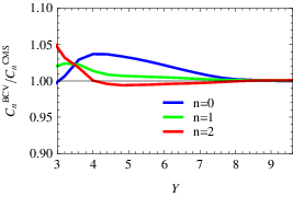
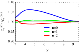
Conceptually, this is a big difference. However, we have to remember that, since the MN jets have typically a large rapidity distance, it is rather unlikely to have the emission of another parton at even larger absolute rapidities. For this reason, we don’t expect big differences between the two procedures. In practice we find differences of the order of 4% at intermediate rapidities ($Y\simeq 3\div 5$) and much smaller at larger rapidities. Fig. 3 shows the relative difference between the NLL BFKL predictions with the original NLL jet vertices (BCV) and the one with modified jet selection that prevents the emission of a parton with ${\boldsymbol{p}}>35\;\mathrm{GeV}$ and $y>y_{J}$ (CMS). We note that the relative difference almost doubles at 13 TeV, and cannot be neglected.

Let me just mention that it could be possible to modify the experimental analysis of MN jets in order to comply with the original proposal of NLO jet vertices, but we think that it is better to modify the theoretical prescription by requiring the absence of jets with ${\boldsymbol{p}}>35\;\mathrm{GeV}$ and $y>y_{J}$.

Finally, we want to present the matching procedure. We believe that exploiting all the actual knowledge of perturbation theory should produce more reliable results and improve the description of data, with reduced scale uncertainties. Our hope is also to improve the estimate of cross-section, and not just the azimuthal decorrelation. In this case, we think that fixed NLO and probably NNLO corrections must be fully taken into account.

The matching procedure is rather standard, though tricky at some point, as you will see. In practice, we add to BFKL the full perturbative NLO result, and then subtract the $\mathcal{O}\left(\alpha_{\mathrm{s}}^{3}\right)$ part already included in BFKL, in order to avoid double counting. The implementation is still work in progess, therefore we can show only preliminary results of central values, without error estimate yet. However, we can learn an important lesson for future phenomenological analysis.

Let me start with the computation of the differential cross-section with respect to the rapidity difference of the two jets. Here the center-of-mass energy is 7 TeV and we impose symmetric cuts on the two jet transverse momenta, as in the CMS analysis. In fig. 4 we show the NLL BFKL prediction in green, and compare it with the fixed NLO result in red. The latter turns out to be negative! Furthermore, after several days of computing time, MC-integration errors are still large, due to the slow convergence of the integrand. However, also the double-counting subtraction (purple) is negative. Since the difference between red and purple is moderate, the matched cross-section (blue) receives a moderate correction and remains positive.

An analogue behaviour is shared by the first azimuthal coefficient $C_{1}$. The matching procedure provides moderate but definitely sizeable corrections, in particular at intermediate values of $Y$.

Let me briefly discuss the issue of negative cross-section and instability of jet cross-section with symmetric cuts. It is well known that jet cross-sections at NLO are very sensitive to the asymmetry parameter $\Delta$ which measures the imbalance between the ${\boldsymbol{p}}$-cuts on the two jets. Despite the fact that NLO cross-sections are finite for all values of $\Delta$, they are affected by a $\Delta\log(\Delta)$ singularity of collinear origin, which provides an infinite derivative at $\Delta=0$, that is with symmetric jet cuts, and even negative cross-sections for small $\Delta$-values, as we have seen.

However, and analogous singularity occurs in the subtraction term, as can be seen in the expansion of the BFKL cross-section. It turns out that in the matching procedure such singular terms cancel out to a large extent, so that the matching is quite safe.

Actually, this problem could be avoided by using asymmetric cuts on the jet transverse energies, but this introduces an unpleasant asymmetry. Fortunately, there is another way to avoid (or at least to reduce) this problem while keeping symmetry between the two jets, that is to impose a cut on the average jet transverse energy: $\frac{1}{2}(|{\boldsymbol{p}}_{1}|+|{\boldsymbol{p}}_{2}|)>E_{\mathrm{cut}}$. In this case, also the fixed-order cross-section is well behaved, and the whole procedure is more stable than the previous one, as shown in fig. 5. The same is true for the $C_{1}$ angular coefficient.

For this reason, we strongly suggests experimentalists to perform MN jets analysis with a cut on the average of the jet transverse energies, as already done in other jet analysis. This allows smaller theoretical uncertainties so that MN jets become a better tool for finding evidence of BFKL dynamics, which at present energies is still competing with fixed order contributions, even at LHC.

To conclude, MN jets are a good observable for demonstrating the presence of BFKL dynamics at high energy, with yet open questions to be answered. Fixed order MC and NLL BFKL descriptions are quite different, in some cases close to data, but the overall agreement is not good.

We observed that the theoretical formulation of jet vertices has to be modified in order to comply with the experimental analysis that identifies as MN jets those with the largest rapidity separation. We propose an improved theoretical description of MN jets based on matching BFKL resummed calculations with fixed-order ones. We have computed various observables and we will provide a full analysis with estimates of theoretical uncertainties.

We think that a precise experimental analysis from the 13 TeV run would be very valuable for the study of QCD at high energies. In this respect, we strongly suggest experimentalists of LHC to carry out such analysis by imposing different cuts on the jet transverse momenta, for instance a cut on the average transverse energy of jets.

References

- [1] A. H. Mueller and H. Navelet, Nucl. Phys. B 282 (1987) 727. doi:10.1016/0550-3213(87)90705-X
- [2] V. S. Fadin, E. A. Kuraev and L. N. Lipatov, Phys. Lett. B 60 (1975) 50; E. A. Kuraev, L. N. Lipatov and V. S. Fadin, Sov. Phys. JETP 44 (1976) 443 [Zh. Eksp. Teor. Fiz. 71 (1976) 840] [Erratum-ibid. 45 (1977) 199]; E. A. Kuraev, L. N. Lipatov and V. S. Fadin, Sov. Phys. JETP 45 (1977) 199 [Zh. Eksp. Teor. Fiz. 72 (1977) 377]; I. I. Balitsky and L. N. Lipatov, Sov. J. Nucl. Phys. 28 (1978) 822 [Yad. Fiz. 28 (1978) 1597].
- [3] J. Bartels, D. Colferai and G. P. Vacca, Eur. Phys. J. C 24 (2002) 83 [hep-ph/0112283]; J. Bartels, D. Colferai and G. P. Vacca, Eur. Phys. J. C 29 (2003) 235 [hep-ph/0206290].
- [4] D. Colferai, F. Schwennsen, L. Szymanowski and S. Wallon, JHEP 1012 (2010) 026 [arXiv:1002.1365 [hep-ph]].
- [5] CMS Collaboration [CMS Collaboration], CMS-PAS-FSQ-12-002.
- [6] B. Ducloué, L. Szymanowski and S. Wallon, JHEP 1305 (2013) 096 [arXiv:1302.7012 [hep-ph]].
- [7] S. J. Brodsky, G. P. Lepage and P. B. Mackenzie, Phys. Rev. D 28 (1983) 228. doi:10.1103/PhysRevD.28.228
- [8] F. Caporale, D. Y. Ivanov, B. Murdaca and A. Papa, Eur. Phys. J. C 74 (2014) no.10, 3084 Erratum: [Eur. Phys. J. C 75 (2015) no.11, 535] doi:10.1140/epjc/s10052-014-3084-z, 10.1140/epjc/s10052-015-3754-5 [arXiv:1407.8431 [hep-ph]].
- [9] F. Caporale, D. Y. Ivanov, B. Murdaca, A. Papa and A. Perri, JHEP 1202 (2012) 101 doi:10.1007/JHEP02(2012)101 [arXiv:1112.3752 [hep-ph]].