Phase Transitions in a Logistic Metapopulation Model with Nonlocal Interactions

In developing our model, we consider our habitat as a portion of the earth on which species are able to colonize and live. Considering a habitat that lie along a lake or pond and subdividing it into distinct patches enables us to consider a one dimensional periodic habitat $S.$ We label each site in this habitat by an integer and denote the set of these integers by ${S}:=\{0,1,\cdots,N-1\}.$ We denote by $p_{n}$ the population density at site n and introduce the vector notation $\mathbf{p}:=(p_{n})_{n\in S}=(p_{0},p_{1},\cdots,p_{N-1})$. Following Smith (2007); Mandal and Asif (2007), discrete Fourier series (DFS) of this vector is denoted by $\mathcal{F}\mathbf{p}=\mathbf{P}=(P_{k})_{k\in S}$ and given by

for any $k\in S.$ Note that $j$ is used to denote the imaginary unit number.

Define the componentwise multiplication (or Hadamart product) of two vectors $\mathbf{x}$ and $\mathbf{y}$ as

Thus in accordance with this definition of multiplication, any power of vector $\mathbf{x}$ can be defined by

Additionally, we consider the vector of complex exponentials $\mathbf{w}=\bigl(e^{2\pi jn/N}\bigr)_{n\in S}.$ For integers $m_{1}$ and $m_{2},$ we have the following orthogonality property of complex exponential vectors:

where $\cdot$ is the inner product of two vectors in $\mathbb{C}^{N}.$ This property follows from the discussion by Smith (2007, p. 104). Moreover, we would like to note that the set $\{\mathbf{w}^{m}|m=0,1,\cdots,N-1\}$ is a basis for the vector space $\mathbb{C}^{N}.$

Lastly, denote the discrete convolution operator of two vectors $\mathbf{x}$ and $\mathbf{y}$ by $\mathbf{x}*\mathbf{y}$ and define it as follows:

where ${<i-n>_{N}}=i-n\penalty\ \text{modulo}\penalty\ N.$ It can be seen that the DFS of the convolution of two vectors $\mathbf{x}$ and $\mathbf{y}$ is given by the Hadamart product of DFS of these vectors i.e. we have:

For a review of these results, see Smith (2007); Mandal and Asif (2007).

Consider our one dimensional periodic habitat $S.$ If an individual with site of origin $n$ adopts another site $i$ for residence, this movement is called the dispersal from site $n$ to site $i$. One can chose to model such movements between discrete patches of this habitat by discrete dispersal or island chain models (Levin 1974; Hastings 1978; Cantrell and Cosner 2003). Such models can be set in either discrete or continuous time (Cantrell and Cosner 2003). Following Levin (1974) and Hastings (1978), we consider a continuous time model. Suppose that in each patch the population grows or declines according to a differential equation $dp_{n}/dt=f_{n}(\mathbf{p})$ where $\mathbf{p}=(p_{n})_{n\in S}.$ Next we describe how the population density $p_{i}$ on each patch $i\in S$ varies in time.

Here we consider passive dispersal of individuals between patches which is quantified in terms of two major parameters: (1) dispersal rate is the expected proportion of individuals to leave a patch and (2) dispersal range or distance is usually described by a discrete dispersal kernel which gives the probability distribution of the distance traveled by an individual to find a new breeding site (Matthysen 2012). Suppose that individuals disperse from patch $n$ at a rate of $\delta_{n}\geq 0$ and arrive at patch ${i}$ at a rate of ${\tilde{d}_{in}\geq 0}.$ Hence our model is given as follows:

with $\delta_{n}={\sum_{i\in S}\tilde{d}_{ni}}$ which implies that there is no mortality in transit. Suppose also that the dispersal rates depend on the distance between two sites $i$ and $n$ i.e. we have:

Hence, the summation in equation (1) defines a circular convolution as follows:

This also implies that the dispersal rates satisfies $\delta:=\delta_{n}$ for any $n\in S.$

Hastings (1978); Levin (1974) assumed that the growth rate of the population at a site depends only on the population density at the same patch. However, Britton (1989) and Doebeli and Killingback (2003) criticized this assumption and claimed that the population growth depends not only on the resources in the local patch but also on the resources in neighboring spatial locations. One can consider, for instance, situations in which reproduction and hence population dynamics take place in a habitat patch whose resources are also used by individuals that live and reproduce in neighboring patches through foraging. Therefore the depletion of resources in a given habitat patch occurs not only due to the individuals living and reproducing in this patch, but also due to individuals living in a certain neighborhood of that patch. Vegetation dynamics is another interesting example in which nonlocal competition appears to be occurring (Lefever and Lejeune 1997; von Hardenberg et al. 2001; Maruvka and Shnerb 2006). Since water is a diffusible resource it follows that the effect of a plant consuming water locally is that it consumes water from the surrounding regions. Thus the greater the rate of water uptake by a given biomass at a patch, the lower the quantity of water available at neighboring patches implying that nearby patches with low soil moisture may be hostile for a new agent. In this example, the vegetation dynamics is governed by local resource uptake, yet nonlocal competition results from the diffusion of the resource. Hence, we consider nonlocal coupling between habitat patches taking into account not only dispersal between neighboring patches but also nonlocal interactions.

Taking into account research conducted by Britton (1989) and Doebeli and Killingback (2003), we assume that the resources available to an individual is given by the spatial average of the resources in a certain neighborhood of the breeding site of the individual. Considering logistic growth and following the model setup presented by Genieys et al. (2006) lead us to the following growth rate of the population at site $n$:

where $a_{n}$ is the carrying capacity of site $n$ and $\mathbf{c}$ is the nonlocal competition kernel. Sasaki (1997) analyzed the continuous space analog of this equation with slowly varying carrying capacity in space variable and concluded that the model exhibits very complicated dynamics. Since we want to analyze the behavior of patterns in terms of their amplitudes, we have a simplifying assumption that is given by $a_{n}=1$ for all $n\in S.$ This is to say that each patch is identical; hence, $\mathbf{p}=\mathbf{1}$ is the space homogenous solution of the equation.

Thus, we get the following system of differential equations

where both $\mathbf{d}$ and $\mathbf{c}$ are discrete probability distributions on $\mathbb{Z}$ (or simply on $S$). The functions $f_{n}$ defined in (2) are non-dimensionalized for time; in other words, equation (3) has been scaled in time so that $\delta$ is the relative time scale between dispersal and reproduction. We remark that the above given model mimics the nonlocal Fisher equation (Britton 1989; Gourley 2000) in a patchy environment.

We summarize the above given assumptions regarding our model as follows:

• (A1)

  Regarding the dispersal kernel $\mathbf{d}$, we have assumed that it is a probability distribution on $S$ describing the proportion of individuals dispersing from one site to another by accounting the distance between them. Biologically, this implies that individuals are not lost or do not reproduce while dispersing. In addition, unless the kernel is degenerate (i.e. $d_{0}=1$) the descendants of an individual from a site $i$ can be found in any site in $S$ after enough generations. The dispersal between two spatial locations is assumed to depend on the distance between them due to the limited mobility of individuals.

• (A2)

  Regarding the competition or interaction kernel $\mathbf{c},$ we have assumed that it satisfies the same assumptions with the dispersal kernel. This kernel was used to calculate average frequency of the species, competing for the common resources, in a neighborhood of any spatial location. Since competition is restricted to a neighborhood, it is also realistic to assume that this kernel takes the spatial distance between sites into account.

• (A3)

  Regarding the reproduction term $f_{n}(\mathbf{p})$, we have assumed that it is a modified logistic growth function. We would like to note that this growth term can be obtained by specifying birth and death rates of the species (see Genieys et al. (2006, section 2)). Biologically, this growth term implies that the more offspring are produced in a patch as the population gets larger in the site. Whereas the reproduction and survival decrease in a site as the average density of individuals increases in the neighborhood of the site. The latter is due to the fact that the carrying capacity affects only the average population in the neighborhood of any patch in our model. This also implies that the population size may exceed the carrying capacity in some spatial patches provided that the average population size is small enough.

If we assume that there is no spatial effect i.e. $d_{0}=c_{0}=1$ , (3) becomes the simple logistic equation with stable solution $p_{n}=1$ for all $n\in S.$

To investigate necessary conditions for pattern formation, we linearize (3) by using the first order expansion $\mathbf{p}=1+\varepsilon\check{\mathbf{p}}e^{\lambda t},$ where $\check{\mathbf{p}}$ is a spatial perturbation term independent of time $t.$ Hence this formula can be considered as a separation of variables formula for (3). Substituting this ansatz to the equation gives the following first order relation:

By taking the DFS of both sides, one gets

where $\mathbf{D}=(D_{k})_{k\in S}$ and $\mathbf{C}=(C_{k})_{k\in S}$ are DFS of probability kernels $\mathbf{d}$ and $\mathbf{c},$ respectively. Here we would like to note that the Fourier transforms (or characteristic functions) of these kernels can take complex values since the kernel functions are not necessarily symmetric. Therefore, we introduce notations $\mathcal{R}[z]$ and $\mathcal{I}[z]$ to denote real and imaginary parts of a complex number $z,$ respectively.

Note that stability condition for the equilibrium $\mathbf{1}$ is given as $\mathcal{R}[\lambda(\delta,k)]<0$ for all $k\in S.$ Since kernel $\mathbf{d}$ is a discrete probability distribution, $\mathcal{R}\big[{\mathbf{D}}-\mathbf{1}\big]\leq 0$ for the dispersal kernel. This implies that we need to require $\mathcal{R}[{C_{k}}]<0$ for some $k\in S$ to destabilize steady state $\mathbf{p}=\mathbf{1}.$ The effects of nonlocal dispersal and competition are now more apparent. Increasing the dispersal rate between patches flattens the spatial heterogeneity (or it may have no effect on the stability of the equilibrium, see Assumption 3.1). This is to say that the spatial inhomogeneity arises as a result of nonlocal averaging.

Define the set $\tilde{S}=\{k\in S:\mathcal{R}[{C_{k}}]<0\}.$ If the DFS of the dispersal kernel $D_{k}$ is equal to 1 for some $k\in\tilde{S}$ then the state $\mathbf{1}$ is unstable for any positive dispersal rate $\delta.$ To proceed and define the critical dispersal rate we need the following assumption.

Hereafter we always require that Assumption 3.1 holds. This assumption is not a requirement to observe spatially inhomogeneous solutions but it rules out some kernels for which dispersal loses its flattening effect. Hence it guarantees the existence of a positive dispersal rate at which spatial homogeneity vanishes. This rate will be used as a bifurcation point for the further analysis of the model. Note that this assumption is not redundant, yet the discussion is rather technical and given in Appendix A.2.

One can easily conclude that steady state $\mathbf{p}=\mathbf{1}$ is unstable for $\delta=0$ as long as $\mathcal{R}[C_{k}]<0$ for some $k\in S.$ By continuity, it is also unstable for small enough $\delta>0.$ By Assumption 3.1, $\mathcal{R}[D_{k}-1]<0$ for any $k\in\tilde{S}.$ Hence, for large enough $\delta>0$ the state will be stable. The critical dispersal rate $\delta_{0}$ is calculated by solving the following maximization problem:

We denote the argument of the maximization problem by $k_{c}$ which is called the critical wavenumber. We remark that the critical wave number $k_{c}$ is in the set $\tilde{S}.$

Here we focus on instabilities around stability boundaries. Our numerical simulations show that only stationary and traveling waves can be observed near stability boundaries (for an illustration of these patterns see Figure 2 Panels (a) and (b), respectively ).

It has been shown that the solutions to nonlocal Fisher equation exhibit pattern formation if the real part of the characteristic function of nonlocal contact term takes negative values (Genieys et al. 2006). Hence, symmetric uniform kernels have been used widely to model nonlocal interactions (see for example Fuentes et al. (2003); Fuentes et al. (2004); Genieys et al. (2006)). Following recent works by Segal et al. (2013); Tanzy et al. (2013); Aydogmus (2015), we assume that each convolution term depends on two parameters. $r_{d}$ and $a_{d}$ characterize the range of nonlocality and extent of asymmetry for dispersal kernel $\mathbf{d},$ respectively. Similarly, $r_{c}$ and $a_{c}$ characterize the range of nonlocality and extent of asymmetry for interaction kernel $\mathbf{c},$ respectively. Taking $a_{i}=0$ for $i=d$ or $c$ implies that the corresponding kernel is symmetric. As an example, one can consider the family of step functions for positive integers $a$ and $r$ as follows:

for $n\in\mathbb{Z}.$ Note that equation (7) is an infinite sequence which is denoted by $\mathbf{v}_{\infty}^{(r,a)}:=\big(v_{n}^{(r,a)}\big)_{n\in\mathbb{Z}}.$

For the sake of simplicity, we assume assume that $2r+1\leq N.$ Hence, (7) can be considered as an $N$ dimensional vector which is denoted by $\mathbf{u}^{(r,a)}$ with $u_{n}^{(r,a)}:=v_{<n>_{N}}^{(r,a)}.$ The DFS of the uniform kernel $\mathbf{u}^{(r,a)}$ is calculated in Appendix (A.1). We remark that discrete uniform kernel (7) is a discretization of the top-hat kernel used to model nonlocal dispersal for continuous space ecological processes (Lutscher 2007).

We consider two examples for $N={17}$ as follows:

• E1:

  Stationary waves, in Figure 2 (a), were obtained for the parameters $\mathbf{d}=\mathbf{c}=\mathbf{u}^{(1,0)}$ (see Figure 1 Panel (K1)), initial condition $1+0.001\cos(k_{c}x)$ and $\delta=0.2435$ while the critical value of the nonlocal dispersal rate is given by $\delta_{0}=0.2436.$

• E2:

  Figure 2 (b) shows periodic traveling waves obtained for the kernel functions $\mathbf{d}=\mathbf{u}^{(2,0)}$ and $\mathbf{c}=\mathbf{u}^{(5,2)}$ (see Figure 1 Panels (K2) and (K3), respectively), initial condition $1+0.001\cos(k_{c}x)$ and the dispersal rate is taken as the critical nonlocal dispersal rate i.e. $\delta=\delta_{0}=0.1103.$

Our biological motivation for considering these two examples are as follows. In example E1, we assumed that competition for resources occurs not only between individuals in a given patch, but also to some extent between individuals reproducing in neighboring patches to which individuals may leave their home territory in search of food. In the second example $\textbf{E2},$ on the other hand we assumed that the interaction range is larger than the dispersal range. Juxtacrine cell signaling can be considered as an example for which nearest neighborhood signaling mechanism account for the observed increase in cell proliferation many cell diameters away from the wound edge Monk et al. (2001). For some plant populations, this assumption might also be relevant. In the case of vegetation dynamics studied by Lefever and Lejeune (1997), for example, the range of inhibitory effect of nonlocal water consumption is assumed to be larger than the dispersal distance. In the same study it was also assumed that the interaction kernel is isotropic i.e. slope imposing to rainwater is a well-defined running down direction. We can relax this assumption and consider an environment with anisotropy. This relaxation leads us to consider asymmetric nonlocal competition which may be modeled by using a discrete asymmetric kernel (see, Figure 1 Panel (K3)).

Figure 1 (a) shows the stationary wave-type patterns obtained using parameters given in E1. Figure 1 (b), on the other hand, shows periodic traveling waves that were obtained for the kernel functions and parameters described in E2. It is clear from the Figure 2 that at some patches the population level exceeds the carrying capacity $\mathbf{1}$ while at some others it remains below the carrying capacity as expected (see Section 2, Assumption (A3)). This is to say that individuals form clusters or groups. We would like to note that standing wave-type patterns arises when both interaction and dispersal kernels are symmetric and these groups does not move in space as time passes. If the model takes asymmetric dispersal or interaction into account then traveling wave-type patterns arises and these clusters moves in space.

Here, we would like to call attention to another significant difference between Figure 2 (a) and (b). Recall the discussion on supercritical and subcritical bifurcations in Section 1. From the color bars of these figures, it is possible to see that the amplitudes of stationary and traveling wave solutions are qualitatively different from each other even though each dispersal rate is very close to the corresponding critical dispersal rate. Define the half amplitude of equation (3) as follows:

for a sufficiently large $t^{*}.$ For the stationary waves, we numerically obtained the amplitude of the solution $\text{Amp}^{sw}=0.058.$ Similarly, we got $0.9684\leq\text{Amp}^{tw}\leq 0.9975$ for the traveling waves amplitude of which oscillates in time (see Figure 4, Panel (b)). Our numerical results, therefore, indicate that continuous and discontinuous transitions to instability for the parameters given in E1 and E2, respectively. To further investigate the qualitative difference between transitions to instability, we use weakly nonlinear analysis in Section 4.

We are interested in the stability of the homogenous solution $\mathbf{p}=\mathbf{1}$ near the critical nonlocal dispersal rate $\delta_{0}$ with periodic boundary conditions. We aim to find a solution to weakly nonlinear approximation to (3) by multiple-scales perturbation expansion. Before proceeding to this expansion, we consider a perturbation of the bifurcation parameter $\delta$ as

for $0<\varepsilon\ll 1$ and $\mu=\pm 1.$ Here $\mu$ determines the direction of the deviation from the critical nonlocal dispersal rate $\delta_{0}.$ Note that $\mathbf{p}=\mathbf{1}$ is unstable if $\mu=-1$ by the linear stability analysis presented in Section 3.1

Let $\delta_{0}$ be the critical dispersal rate for which we have $\lambda(\delta_{0},k_{c})=0.$ The solution to the linearization of (3) around $\mathbf{1}$ and near critical dispersal rate is given as follows:

where $c.c.$ stands for complex conjugate and $\mathbf{w}$ is as defined in Section 2.

Denote the imaginary part of the eigenvalue associated with the critical wavenumber by $w_{0}:=\mathcal{I}[\lambda(\delta_{0},k_{c})].$ Expanding the eigenvalue $\lambda(\delta,k_{c})$ in power series leads to

where we used equality (5) to obtain $\partial\lambda/\partial\delta.$ By substituting this expansion to the above given solution (10), one obtains

Hence amplitude $A$ is a function of the slow time $\tau:=\varepsilon^{2}t.$ We consider the fast and slow time scales $t$ and $\tau$ together in our analysis i.e. $t\to t+\tau.$

Consider the family of linear waves in discrete space as follows:

for $m\in S$ and assume the following formal expansion:

where

Plugging the solution (12) in (3) leads to the following cubic S-L equation:

where coefficients $\Phi$ and $\Psi$ are explicitly given by formulas (20) and (21) along with the details of the derivation of (13) in Appendix B. Note also that equation (13) is valid only if Assumption B.1 is satisfied.

Since solutions to amplitude equations (13) are complex, one can redefine this amplitude function as $A(\tau)=L(\tau)e^{i\theta(\tau)}$ with real terms $L(\tau)=|A(\tau)|$ and $\theta(\tau).$ Hence, an equivalent form of equation (13) is given as follows:

Equilibria of the equation (14) are $L_{0}=0$ and $L_{1}=\sqrt{-\mu\mathcal{R}[\Phi]/\mathcal{R}[\Psi]}$ provided that $\mathcal{R}[\Psi]\neq 0.$ If this is not true then the amplitude equation (14) becomes linear. In this case, higher order correction terms are needed to approximate the amplitude levels of pattens. One can easily see that the solution $0$ of (14) is stable whenever $\mu\mathcal{R}[\Phi]<0.$ Thus, it is clear from (20) that equilibrium $\mathbf{p}=\mathbf{1}$ (or $L_{0}$) is unstable for $\mu=-1$ and it is stable for $\mu=1.$ This result is in accordance with the result of the linear analysis given in Section 3.1

It is clear that the equilibrium $L_{1}$ needs to be real i.e. $\mu\mathcal{R}[\Psi]\geq 0.$ Thus the sign of $\mathcal{R}[\Psi]$ determines the direction of deviation from bifurcation parameter. One can categorize the possible bifurcations arising from (14) as follows:

1. 1.

   If $\mathcal{R}[\Psi]>0,$ then $\mu=-1$ and (14) describes a supercritical bifurcation with stable branch $\varepsilon L_{1}$ to the left of $\delta_{0}.$

2. 2.

   If $\mathcal{R}[\Psi]<0,$ then $\mu=1$ and (14) describes a subcritical bifurcation with unstable branch $\varepsilon L_{1}$ to the right of $\delta_{0}.$

Here, the first case implies that a supercritical pitchfork bifurcation arises from the constant density state $\mathbf{p}=\mathbf{1}$ to a spatially periodic pattern with a steady state amplitude determined by $L_{1}.$ In the second case, transitions to instabilities are discontinuous and $L_{1}$ determines the maximum amplitude of the initial conditions above which $\mathbf{p}=\mathbf{1}$ is unstable. In the case of supercritical transitions, it is clear that spatially periodic patterns arises only if the dispersal rate of the population is less than the critical dispersal rate. In addition, amplitude levels as a measure of the spatial fluctuations or cluster sizes increases as mobility of individuals decreases. In the case of subcritical bifurcations, on the other hand, we only obtained an unstable branch for the values of dispersal rates that are larger than the critical dispersal rate. We will investigate this case in more detail computationally and analytically in the remainder of this section.

To further analyze the model, we need to consider higher order correction terms. To accomplish such a task, we take the complex amplitude as a function of two time scales $A(\tau,\tau_{1})$ where the second time scale is given by $\tau_{1}=\varepsilon^{4}t$ and take the bifurcation parameter $\delta$ as

In the case of discontinuous transitions to instability, we need to expand the equations up to fifth order. The calculations are given explicitly in Appendix C. A quintic equation for the partial derivative $A_{\tau_{1}}$ is given by (25). Using this equation along with the equation (13), one can obtain the following quintic S-L equation:

For the derivation of this equation see Appendix C where we also give explicit expressions for parameter values $\Theta_{3}$ and $\Theta_{5}$ (see formulas (26) and (27)). Note also that this equation is only valid if both of the Assumptions B.1 and C.1, given in Appendices B and C, hold. Again the amplitude function $A$ is complex valued. Hence we write it as $A(\tau)=L(\tau)e^{i\theta(\tau)}$ with real terms $L(\tau)=|A(\tau)|$ and $\theta(\tau).$ Plugging this equality in quintic S-L equation (16) one obtains:

We are interested in the real roots of RHS of equation (17). Equilibrium $L_{0}=0$ is again unstable for $\mu=-1$ and it is stable for $\mu=1.$

The RHS of (17) has four roots other than zero determined by

Hence we have the following classifications regarding the equilibria of (17) and approximations to the amplitudes of the patterns.

Case 1: Suppose that $\mu=1.$ Then (17) has four real roots other than zero and these roots are symmetric around zero. Consider only the positive roots and denote them by $L_{+}$ and $L_{-}.$ Then the unstable branch can be approximated by $\varepsilon L_{-}$ to the right of $\delta_{0}.$ In addition, $\varepsilon L_{+}$ approximates the stable branch.

Case 2: Suppose that $\mu=-1.$ Then (17) has only two real roots other than zero which are symmetric around zero. There is no unstable branch here, and one can approximate the stable branch by $\varepsilon L_{+}.$

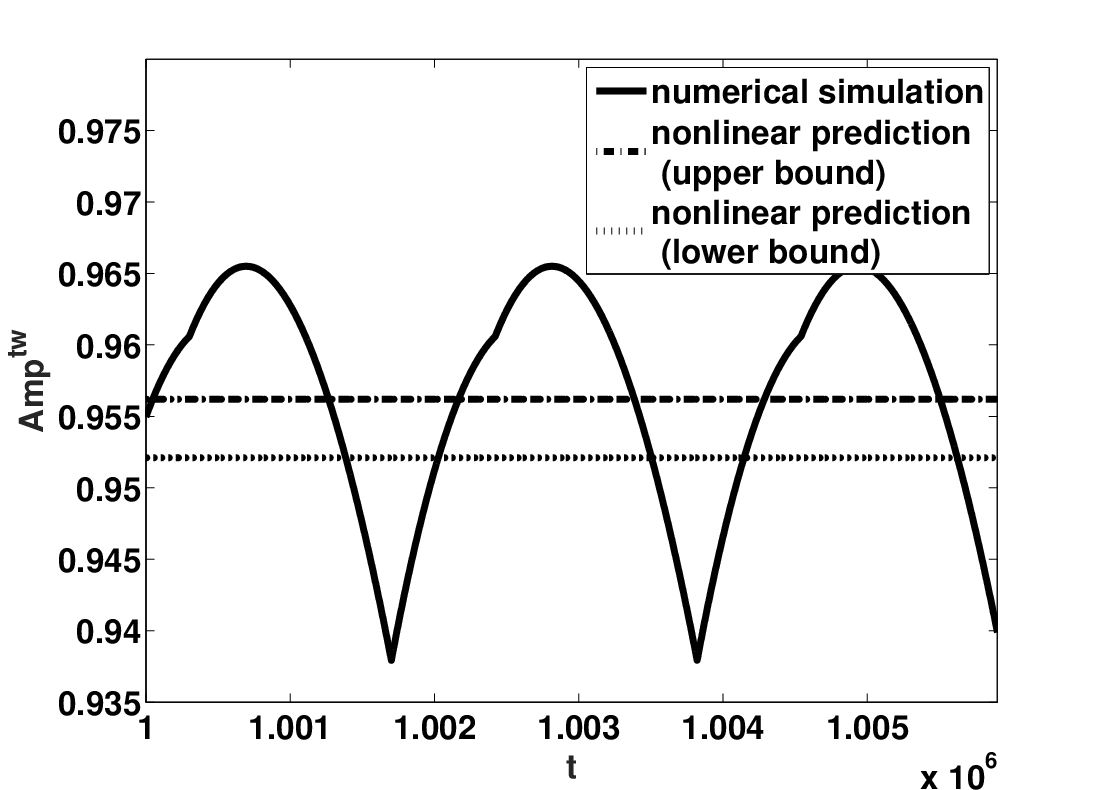
The unstable branch (dashed curve) shown in Figure 4 Panel (a) is calculated using the root $L_{-}=2.8046$ rather than $L_{1}=2.7155$ for the parameters given in E2. The curve again determines the maximum amplitude of initial conditions below which the space homogenous equilibrium $L_{0}$ is reached. If the amplitude of the initial condition passes this maximum value then one can observe pattern formation whose amplitude levels are obtained numerically (black dots). An approximation of stable amplitude levels is given by the black curve for $f(t^{*})=1.99$. Note that the approximation stays relatively close to numerically obtained amplitude levels (black dots) when $\delta$ is close enough to $\delta_{0}.$ Yet as the distance between $\delta$ and $\delta_{0}$ increases, the approximation fails to capture the numerically obtained amplitude levels since the magnitude of error term is given by $O\Bigl(\sqrt{|\delta-\delta_{0}|}\Bigr)$ (see Remark 2). Quintic SL equation mainly predicts the maximum difference between the densities of the residents living in different patches. Hence this approximation informs us about the degree of spatial inhomogeneity. Another observation is that decreasing the dispersal rate leads more denser group of individuals as in the case of supercritical bifurcations.

In Panel (b), the actual amplitude levels of the patterns are plotted as a function of time $t$ for dispersal rate $\delta=0.1104.$ The upper and lower bounds are calculated using weakly nonlinear predictions for the values $f(t^{*})=1.9830\text{ and }1.9915,$ respectively.

References

- Aydogmus (2015) O Aydogmus. Patterns and transitions to instability in an intraspecific competition model with nonlocal diffusion and interaction. Math. Mod. Nat. Phen., 10(6):17–29, 2015.
- Aydogmus et al. (2017) O Aydogmus, Y Kang, M E Kavgaci, and H Bereketoglu. Dynamical effects of nonlocal interactions in discrete-time growth-dispersal models with logistic-type nonlinearities. Ecol. Complexity, 31:88–95, 2017.
- Banerjee and Volpert (2016a) M Banerjee and V Volpert. Spatio-temporal pattern formation in rosenzweig–macarthur model: Effect of nonlocal interactions. Ecol. Complexity, 2016a.
- Banerjee and Volpert (2016b) M Banerjee and V Volpert. Prey-predator model with a nonlocal consumption of prey. Chaos, 26(8):083120, 2016b.
- Banerjee et al. (2016) M Banerjee, V Vougalter, and V Volpert. Doubly nonlocal reaction-diffusion equation and the emergence of species. arXiv preprint arXiv:1601.04257, 2016.
- Beekman et al. (2001) M. Beekman, DJT Sumpter, and FLW Ratnieks. Phase transition between disordered and ordered foraging in pharaoh’s ants. Proc. Nat. Acad. Sci., 98(17):9703–9706, 2001.
- Britton (1989) NF Britton. Aggregation and the competitive exclusion principle. J. Theor. Biol., 136(1):57–66, 1989.
- Britton (1990) NF Britton. Spatial structures and periodic travelling waves in an integro-differential reaction-diffusion population model. SIAM J. App. Math., 50(6):1663–1688, 1990.
- Cantrell et al. (2012) R S Cantrell, C Cosner, and W F Fagan. The implications of model formulation when transitioning from spatial to landscape ecology. Math. Biosci. and Eng., 9(1):27–60, 2012.
- Cantrell and Cosner (2003) RS Cantrell and C Cosner. Spatial ecology via reaction-diffusion equations. John Wiley & Sons, 2003.
- Cobbold et al. (2015) CA Cobbold, F Lutscher, and JA Sherratt. Diffusion-driven instabilities and emerging spatial patterns in patchy landscapes. Ecol. Complexity, 24:69–81, 2015.
- Doebeli (1995) M Doebeli. Dispersal and dynamics. Theor. Pop. Biol., 47(1):82–106, 1995.
- Doebeli and Killingback (2003) M Doebeli and T Killingback. Metapopulation dynamics with quasi-local competition. Theor. Pop. Biol., 64(4):397–416, 2003.
- Durrett and Levin (1994) R Durrett and SA Levin. The importance of being discrete (and spatial). Theor. Pop. Biol., 46(3):363–394, 1994.
- Eftimie et al. (2009) R Eftimie, G de Vries, and MA Lewis. Weakly nonlinear analysis of a hyperbolic model for animal group formation. J. Math. Biol., 59(1):37–74, 2009.
- Fuentes et al. (2003) MA Fuentes, MN Kuperman, and VM Kenkre. Nonlocal interaction effects on pattern formation in population dynamics. Phys. Rev. Lett., 91(15):158104, 2003.
- Fuentes et al. (2004) MA Fuentes, MN Kuperman, and VM Kenkre. Analytical considerations in the study of spatial patterns arising from nonlocal interaction effects. J. Phys. Chem. B, 108(29):10505–10508, 2004.
- Genieys et al. (2006) S Genieys, V Volpert, and P Auger. Pattern and waves for a model in population dynamics with nonlocal consumption of resources. Math. Mod. Nat. Phen., 1(01):63–80, 2006.
- Gilpin and Hanski (1997) M Gilpin and I Hanski. Metapopulation biology: ecology, genetics, and evolution. Academic Press, 1997.
- Gourley (2000) SA Gourley. Travelling front solutions of a nonlocal fisher equation. J. Math. Biol., 41(3):272–284, 2000.
- Gyllenberg et al. (1993) M Gyllenberg, G Söderbacka, and S Ericsson. Does migration stabilize local population dynamics? analysis of a discrete metapopulation model. Math. Biosci., 118(1):25–49, 1993.
- Hanski (1994) I Hanski. A practical model of metapopulation dynamics. J. Anim. Ecol., pages 151–162, 1994.
- Hastings (1978) A Hastings. Global stability in lotka-volterra systems with diffusion. J. Math. Biol., 6(2):163–168, 1978.
- Hastings (1993) A Hastings. Complex interactions between dispersal and dynamics: lessons from coupled logistic equations. Ecology, 74(5):1362–1372, 1993.
- Hastings and Harrison (1994) A Hastings and S Harrison. Metapopulation dynamics and genetics. Ann. Rev. Ecol. and Sys., pages 167–188, 1994.
- Holmes et al. (1994) EE Holmes, MA Lewis, JE Banks, and RR Veit. Partial differential equations in ecology: spatial interactions and population dynamics. Ecology, pages 17–29, 1994.
- Hoyle (2006) RB Hoyle. Pattern formation: an introduction to methods. Cambridge University Press, 2006.
- Kisdi and Utz (2005) É Kisdi and M Utz. Does quasi-local competition lead to pattern formation in metapopulations? an explicit resource competition model. Theor. Pop. Biol., 68(2):133–145, 2005.
- Kot (1992) M Kot. Discrete-time travelling waves: ecological examples. J. Math. Biol., 30(4):413–436, 1992.
- Lefever and Lejeune (1997) R Lefever and O Lejeune. On the origin of tiger bush. Bull. Math. Biol., 59(2):263–294, 1997.
- Levin (1974) SA Levin. Dispersion and population interactions. Am. Nat., pages 207–228, 1974.
- Lutscher (2007) F Lutscher. A short note on short dispersal events. Bull. Math. Biol., 69(5):1615–1630, 2007.
- Madras et al. (1996) N Madras, J Wu, and X Zou. Local-nonlocal interaction and spatial-temporal patterns in single species population over a patchy environment. Canad. Appl. Math. Quart, 4:109–133, 1996.
- Mandal and Asif (2007) M Mandal and A Asif. Continuous and discrete time signals and systems. Cambridge University Press, 2007.
- Maruvka and Shnerb (2006) Y E Maruvka and N M Shnerb. Nonlocal competition and logistic growth: patterns, defects, and fronts. Phys. Rev. E, 73(1):011903, 2006.
- Matthysen (2012) E. Matthysen. Multicausality of dispersal: a review. Dispersal ecology and evolution, pages 3–18, 2012.
- Monk et al. (2001) NAM Monk, J A Sherratt, and M R Owen. Spatiotemporal patterning in models of juxtacrine intercellular signalling with feedback. In Mathematical Models for Biological Pattern Formation, pages 165–192. Springer, 2001.
- Murray (2003) JD Murray. Mathematical biology ii: spatial models and biomedical applications, 2003.
- Neubert et al. (1995) MG Neubert, M Kot, and MA Lewis. Dispersal and pattern formation in a discrete-time predator-prey model. Theor. Pop. Biol., 48(1):7–43, 1995.
- Okubo and Levin (2013) A Okubo and SA Levin. Diffusion and ecological problems: modern perspectives, volume 14. Springer Science & Business Media, 2013.
- Owen and Sherratt (1998) M R Owen and J A Sherratt. Mathematical modelling of juxtacrine cell signalling. Math. Biosci., 153(2):125–150, 1998.
- Pachepsky et al. (2005) E Pachepsky, F Lutscher, and MA Lewis. The effect of dispersal patterns on stream populations. SIAM Rev., 47(4):749–772, 2005.
- Sasaki (1997) A Sasaki. Clumped distribution by neighbourhood competition. J. Theor. Biol., 186(4):415–430, 1997.
- Segal et al. (2013) BL Segal, VA Volpert, and A Bayliss. Pattern formation in a model of competing populations with nonlocal interactions. Physica D: Nonl. Phen., 253:12–22, 2013.
- Segel and Stoeckly (1972) LA Segel and B Stoeckly. Instability of a layer of chemotactic cells, attractant and degrading enzyme. J. Theor. Bio., 37(3):561–585, 1972.
- Smith (2007) JO Smith. Mathematics of the discrete Fourier transform (DFT): with audio applicaitons. W3K Publishing, 2007.
- Stuart (1960) JT Stuart. On the non-linear mechanism of wave disturbances in stable and unstable parallel flows. part i. J. Fluid Mech., 9:152–171, 1960.
- Tanzy et al. (2013) MC Tanzy, VA Volpert, A Bayliss, and ME Nehrkorn. Stability and pattern formation for competing populations with asymmetric nonlocal coupling. Math. Biosci., 246(1):14–26, 2013.
- Topaz et al. (2006) CM Topaz, AL Bertozzi, and MA Lewis. A nonlocal continuum model for biological aggregation. Bull. Math. Biol., 68(7):1601–1623, 2006.
- Turing (1952) AM Turing. The chemical basis of morphogenesis. Philos. Trans. R. Soc. London B: Biol. Sci., 237(641):37–72, 1952.
- Utz et al. (2007) M Utz, É Kisdi, and M Doebeli. Quasi-local competition in stage-structured metapopulations: a new mechanism of pattern formation. Bull. Math. Biol., 69(5):1649–1672, 2007.
- von Hardenberg et al. (2001) J von Hardenberg, E Meron, M Shachak, and Y Zarmi. Diversity of vegetation patterns and desertification. Phys. Rev. Lett., 87(19):198101, 2001.