Fully leafed induced subtrees Thanks: A. Blondin Massé is supported by a grant from the National Sciences and Engineering Research Council of Canada (NSERC) through Individual Discovery Grant RGPIN-417269-2013. M. Lapointe is supported by a scholarship CGSD3-488894-2016 from the NSERC and É. Nadeau is supported by a scholarship from the NSERC.
Abstract
Let be a simple graph on vertices. We consider the problem of deciding whether there exists an induced subtree with exactly vertices and leaves in . We study the associated optimization problem, that consists in computing the maximal number of leaves, denoted by , realized by an induced subtree with vertices, for . We begin by proving that the problem is NP-complete in general and then we compute the values of the map for some classical families of graphs and in particular for the -dimensional hypercubic graphs , for . We also describe a nontrivial branch and bound algorithm that computes the function for any simple graph . In the special case where is a tree of maximum degree , we provide a time and space algorithm to compute the function .
1 Introduction
In the past decades, subtrees of graphs, as well as their number of leaves, have been the subject of investigation from various communities. For instance in 1984, Payan et al. [PTX84] discussed the maximum number of leaves, called the leaf number, that can be realized by a spanning tree of a given graph. This problem, called the maximum leaf spanning tree problem (), is known to be NP-complete even in the case of regular graphs of degree [GJ79] and has attracted interest in the telecommunication network community [BCL05, CLR15]. The frequent subtree mining problem [DFBT+14] investigated in the data mining community, has applications in biology. The detection of subgraph patterns such as induced subtrees is useful in information retrieval [Zak02] and requires efficient algorithms for the enumeration of induced subtrees. In this perspective, Wasa et al. [WAU14] proposed an efficient parametrized algorithm for the generation of induced subtrees in a graph.
The center of interest of this paper are induced subtrees. The induced property requirement brings an interesting constraint on subtrees, yielding distinctive structures with respect to other constraints such as in the problem. A first result due to Erdős et al. in 1986, showed that the problem of finding an induced subtree of a given graph with more than vertices is NP-complete [ESS86]. Another similar famous problem in the error-correcting codes community, called snake-in-the-box [Kau58] problem, asks for the length of the longest induced path subgraph in hypercubes and is still open as of today. Similarly self-avoiding walks, or paths, have been investigated in various lattices [BM10, DCS12]. When one adds the constraint of being induced, these walks become thick walks. A particular family of thick walks on the square lattice was successfully investigated in [GPdWd18].
Among induced subtrees of simple graphs, we focus in particular on those with a maximal number of leaves. We call these objects fully leafed induced subtrees (FLIS). Particular instances of the FLIS have recently appeared in the paper of Blondin Massé et al. [BMdCGS18], where the authors considered the maximal number of leaves that can be realized by tree-like polyominoes, respectively polycubes, which are edge connected, respectively face connected, sets of unit square, respectively cubes. The investigation of fully leafed tree-like polyforms led to the discovery of a new 3D tree-like polycube structure that realizes the maximal number of leaves constraint. The observation that tree-like polyominoes and polycubes are induced subgraphs of the lattices and respectively leads naturally to the investigation of FLIS in general simple graphs, either finite or infinite.
To begin with, we consider the decision problem, called leafed induced subtree problem (), and its associated optimization problem, fully leafed induced subtree problem ():
Problem 1.1 ().
Given a simple graph and two positive integers and , does there exist an induced subtree of with vertices and leaves?
Problem 1.2 ().
Given a simple graph on vertices, what is the maximum number of leaves, , that can be realized by an induced subtree of with vertices, for ?
If is an induced subtree of with vertices, we say that is fully leafed when its number of leaves is exactly . Examples of fully leafed induced subtrees are given in Figure 1.
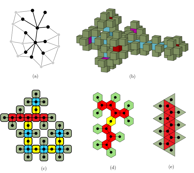
We believe that fully leafed induced subtrees are interesting candidates for the representation of structures appearing in nature and in particular in molecular networks. Indeed, in chemical graph theory, subtrees are known to be useful in the computation of a characteristic of chemical graph, called the Wiener index, that corresponds to a topological index of a molecule [SW05]. The results of [SW05] and [BMdCGS18] suggest that a thorough investigation of subtrees, and in particular induced subtrees with many leaves, could lead to the discovery of combinatorial structures relevant to chemical graph theory.
This paper establishes fundamental results on fully leafed induced subtrees for further theoretical investigations and their applications. First, we prove that the problem is NP-complete. To tackle the problem , we provide a branch and bound algorithm. Contrary to a naive algorithm that considers all induced subtrees to compute the maximal number of leaves, the strategy prunes the search space by discarding induced subtrees that cannot be extended to fully leafed subtrees. When we restrict our investigation to the case of trees, it turns out that the problem is polynomial. To achieve this polynomial complexity, our proposed algorithm uses a dynamic programming strategy. Notice that a naive greedy approach cannot work, even in the case of trees, because a fully leafed induced subtree with vertices is not necessarily a subtree of a fully leafed induced subtree with vertices. All algorithms discussed in this paper are available, with examples, in a public GitHub repository [BMN].
The manuscript is organized as follows. Basic notions are recalled in Section 2 and a proof of the NP-completeness of the decision problem is given. We also study the function in classical families of graphs. A general branch and bound algorithm to compute is described in Section 3. In Section 4, we exhibit a polynomial algorithm to compute the function when is a tree so that the problem is in the class P for the particular case of trees. We conclude the paper in Section 5 with some perspectives on future work.
2 Fully leafed induced subtrees
We recall some definitions from graph theory and refer the reader to [Die10] for fundamental notions. All graphs considered in this text are simple and undirected unless stated otherwise. Let be a graph with vertex set and edge set . Given two vertices and of , we denote by the distance between and , that is the number of edges in a shortest path between and . The degree of a vertex is the number of vertices that are at distance 1 from and is denoted by . We denote by the total number of vertices of and we call it the size of . For , the subgraph of induced by , denoted by , is the graph , where is the set of all subsets of size of . Let be a tree, that is to say, a connected and acyclic graph. A vertex is called a leaf of when . The number of leaves of is denoted by . A subtree of induced by is an induced subgraph that is also a tree.
The next definitions and notation are useful in the study of the and problems.
Definition 2.1 (Leaf function).
Given a finite or infinite graph , let be the family of all induced subtrees of with exactly vertices. The leaf function of , denoted by , is the function with domain defined by
As is customary, we set . An induced subtree of with vertices is called fully leafed when .
Example 2.1.
Consider the graph depicted in Figure 2. Its leaf function is
and the subtree induced by is fully leafed because it has vertices, of them are leaves, and because .
Remark 2.1.
For any simple graph , we have because the empty tree has no leaf, and , since a single vertex is not a leaf. Finally, we always have in any graph with at least one edge.
The following observations are immediate.
Proposition 2.1.
Let be a connected graph with vertices. If is non-isomorphic to , the complete graph on vertices, then .
Proposition 2.2.
For any simple graph with at least 3 vertices, the sequence is non-decreasing if and only if is a tree.
Proof.
If is a tree, then cannot be decreasing because if a subtree of contains a subtree then . If is not a tree, then either contains a cycle or is not connected. In both cases, has no subtree with vertices. Therefore and which implies that there exists a decreasing step in the sequence . ∎
We now describe the complexity of solving the problem .
Theorem 2.1.
The problem of determining whether there exists an induced subtree with vertices and leaves in a given graph is NP-complete.
Proof.
It is clear that is in the class NP. To show that it is NP-complete, we reduce it to the well-known NP-complete problem Independent Set (IndependentSet) [GJ79]: Given a graph and a positive integer , does there exist an independent set of size in , i.e. a subset of vertices that are not pairwise adjacent? Note that an instance of is represented by the tuple where is a graph, the vertex parameter and the leaf parameter. We represent an instance of IndependentSet by the tuple where is a graph and is an integer.
Consider the map that associates to an instance of IndependentSet with , the instance of such that the graph is obtained as with an additional universal vertex , that is linked to each vertex of . Clearly, the map is computable in polynomial time as the graph obtained has vertices and edges.
If is a positive instance of IndependentSet, i.e. an instance for which the answer is yes, then is a positive instance of . Indeed, assume that the graph has an independent set of size . Then these vertices together with the universal vertex is an induced subtree of with vertices and leaves. Conversely, if the instance is a positive instance of , then is a positive instance of IndependentSet. Indeed, assume that contains an induced subtree with vertices and leaves. Observe that the universal vertex cannot be a leaf unless . Consider first that . Then the subtree leaves form an independent set of size of and of . Consider now that . As contains an induced subtree with vertices, has at least one vertex, which is an independent set of size . For , is clearly a positive instance of IndependentSet.
Therefore, IndependentSet and is NP-complete. ∎
From this reduction, we obtain insights on the parameterized complexity of problem. A problem, which is parameterized by , is said to be fixed parameter tractable if it can be solved in time where is the size of the input, is a constant independent from the parameters and is a function of . The class contains all parameterized problems that are fixed parameter tractable. Similarly to the conventional complexity theory, Downey and Fellows introduced a hierarchy of complexity classes to describe the complexity of parameterized problems [DF99]: Since IndependentSet is -complete [DF95a], it follows that is probably fixed parameter intractable. Note that when we replace the induced condition with spanning, the problem becomes fixed parameter tractable [Bod89, DF95b].
Corollary 2.1.
If , then .
We end this section by computing the function for well known families of graphs. First, we consider classical families of finite graphs. Proofs are omitted as they are straightforward.
Complete graphs .
For the complete graph with vertices,
since any induced subgraph of with more than two vertices contains a cycle.
Cycles .
For the cyclic graph with vertices, we have
Wheels .
For the wheel with vertices,
Complete bipartite graphs .
For the complete bipartite graph with vertices,
Hypercubes .
For the hypercube graph with vertices, the computation of is more intricate. Using the branch and bound algorithm described in Section 3 and implemented in [BMN], we were able to compute the values of the function for (see Table 1).
| 0 | 1 | 2 | 3 | 4 | 5 | 6 | 7 | 8 | 9 | 10 | 11 | 12 | 13 | 14 | 15 | 16 | 17 | |
| 0 | 0 | 2 | 2 | * | ||||||||||||||
| 0 | 0 | 2 | 2 | 3 | 2 | * | * | * | ||||||||||
| 0 | 0 | 2 | 2 | 3 | 4 | 3 | 4 | 3 | 4 | * | * | * | * | * | * | * | ||
| 0 | 0 | 2 | 2 | 3 | 4 | 5 | 4 | 5 | 6 | 6 | 6 | 7 | 7 | 7 | 8 | 8 | 8 | |
| 0 | 0 | 2 | 2 | 3 | 4 | 5 | 6 | 5 | 6 | 7 | 8 | 8 | 9 | 9 | 10 | 10 | 11 | |
| 18 | 19 | 20 | 21 | 22 | 23 | 24 | 25 | 26 | 27 | 28 | 29 | 30 | 31 | 32 | 33 | 34 | ||
| * | * | * | * | * | * | * | * | * | * | * | * | * | * | * | ||||
| 11 | 12 | 12 | 13 | 13 | 14 | 14 | 15 | 15 | 16 | 16 | 17 | 17 | 18 | 18 | 18 | * |
Infinite planar lattices.
Blondin Massé et al. have computed the map , where is the regular square lattice with respect to the -adjacency relation [BMdCGS18]:
A similar argument leads to the computation of and for the hexagonal and the triangular lattices:
In the three previous cases, the leaf functions verify linear recurrences. It is therefore easy to deduce that their asymptotic growth is . Notice that the functions and are identical.
The infinite cubic lattice.
The authors of [BMdCGS18] also gave the maximal number of leaves in induced subgraphs with vertices for the regular cubic lattice with respect to the -adjacency relation. This leaf function also satisfies a linear recurrence with asymptotic growth which is slightly larger than for the two-dimensional lattices.
where is the function defined by
3 Computing the leaf function of a graph
We now describe a branch and bound algorithm that computes the leaf function for an arbitrary simple graph . We propose an algorithm based on a data structure that we call an induced subtree configuration.
Definition 3.1.
Let be a simple graph and be a set of colors with coloring functions . An induced subtree configuration of is an ordered pair , where is a coloring and is a stack of colorings called the history of .
All colorings must satisfy the following conditions for any :
- (i)
The subgraph induced by is a tree;
- (ii)
If and , then ;
- (iii)
If , then , where denotes the set of neighbors of .
The initial induced subtree configuration of a graph is the pair where for all and is the empty stack. When the context is clear, is simply called a configuration.
Roughly speaking, a configuration is an induced subtree enriched with information that allows one to generate other induced subtrees either by extension, by exclusion or by backtracking. The colors assigned to the vertices can be interpreted as follow. The green vertices are the confirmed vertices to be included in a subtree. Since each yellow vertex is connected to exactly one green vertex, any yellow vertex can be safely added to the green subtree to create a new induced subtree. The red vertices are those that are excluded from any possible tree extension. A red vertex is excluded by calling the operation ExcludeVertex which is defined below. The exclusion of a red vertex is done either because it is adjacent to more than one green vertex and its addition would create a cycle or because it is explicitly excluded for generation purposes. Finally, the blue vertices are available vertices that have not yet been considered and that could be considered later. For reasons that are explained in the next paragraphs, it is convenient to save in the stack the colorations from which was obtained.
Figure 3(a) illustrates an induced subtree configuration. The green vertices and edges are outlining the induced subtree. The yellow vertices and edges are showing the possible extensions of the green tree. The vertices and are red because each one is connected to two green vertices. Although the vertex is colored in red, it would have been possible to color it in yellow because it is connected to exactly one green vertex. Similarly, vertices , and could be colored either in blue or red since they are not adjacent to the tree.
Let be a configuration of some simple graph , with coloring and stack . We consider the following operations on :
- •
is a non deterministic function that returns any non green vertex in that can be safely colored in green. If no such vertex exists, it returns none. Note that the color of the returned vertex is always , except when , where the color is .
- •
first pushes a copy of on top of , sets the color of to green and updates the colors of the neighborhood of accordingly. Notice that this operation is applied only to a vertex that can be safely colored in green.
- •
first pushes a copy of on top of and then sets the color of to red. This operation is applied only on a vertex such that .
- •
retrieves and removes the top of , then stores it into . In other words, this operation cancels the last operation applied on , which is either an inclusion or an exclusion.
To illustrate these operations, let be the configuration in Figure 3(a). Then could return one of the yellow vertices , , or . Let be the configuration obtained from after calling . Then we have to update the colors of vertices , and by setting , and , as illustrated in Figure 3(b). For any configuration , we call an extension of when its coloration is obtained from without backtracking, i.e. by using only and .
For optimization purposes, it is worth mentioning that it is not necessary to keep a complete copy of the colorations when they are saved in the history . It is sufficient to store the vertex which caused a vertex to become together with a stack of the vertices on which the operations was performed. Keeping this optimization in mind, it is easy to show that the operations and , in the case where the last operation is an inclusion of a vertex , are done in time. Also, the operations and , in the case where the last operation is an exclusion of a vertex , are done in time. Hence, we do not need to copy the whole coloring function at each step, but simply update the neighborhood of some vertex.
It is quite straightforward to use configurations for the generation of all induced subtrees of a graph . Starting with the initial configuration, it is sufficient to recursively build configurations by branching according to whether some vertex returned by the operation is included or excluded from the current green tree. Considering this process as a tree of configurations, the operation can be paired with edges of this tree. Therefore, a careful analysis shows that the generation runs in amortized per solution.
While iterating over all possible configurations, if we want to compute the leaf function , it is obvious that some configurations should be discarded whenever they cannot extend to interesting configurations. Therefore, given an induced subtree configuration of green vertices, we define the function , for , which computes an upper bound on the number of leaves that can be reached by extending the current configuration to a configuration of green vertices. First, the potential is for greater than the size of the connected component containing the green subtree (when computing the connected component, we treat red vertices as removed from the graph). Second, in order to compute this upper bound for , we consider an optimistic scenario in which all yellow and blue vertices that are close enough can safely be colored in green without creating a cycle, whatever the order in which they are selected. Keeping this idea in mind, we start by partitioning the available vertices, which are the yellow and blue vertices together with the leaves of the green tree, according to their distance from the inner vertices of the configuration subtree in . Algorithm 1 computes an upper bound for the number of leaves that can be realized from a configuration of green vertices extended to a configuration of green vertices.
The first part of Algorithm 1 consists in completing the green subtree. More precisely, a configuration is called complete if each yellow vertex is adjacent to a leaf of the green tree. We first verify if is complete and, when it is not the case, we increase and as if the green subtree was completed (Lines 5–9). Next, we choose a vertex among all available vertices within distance . We assume that is green and update and as if all non-green neighbors of were leaves added to the current configuration (Lines 13–17). This process is repeated until the size of the “optimistic subtree” reaches . Note that this process never decreases the values of and . Indeed, in Line 14, the degree of is always greater than since does not exceed the size of the connected component .
Remark 3.1.
We now prove that Algorithm 1 yields an upper bound on the maximum number of leaves that can be realized. It is worth mentioning that, in order to obtain a nontrivial bound, we restrict the available vertices to those that are within distance from the inner vertices of the current green subtree, and then we increase the value of at each iteration.
Proposition 3.1.
Let be a configuration of a simple graph with green vertices and let be an integer such that . Then any extension of to a configuration of vertices has at most leaves, where is the operator described in Algorithm 1.
Proof.
Let be the number of leaves of the green subtree represented by , be the set of inner vertices in the green subtree and
Let . If , then and it is clear that adding vertices cannot add more than leaves.
Otherwise, we proceed by contradiction by assuming that can be extended to a configuration with green vertices and leaves, with . Let be the sequence of vertices that became, in that order, inner vertices in the successive extensions of to reach . Then we have . Let be the vertices chosen by the procedure . It follows from Remark 3.1 that . As we assumed that , we obtain .
Without loss of generality, we assume that if and are at the same distance from and then (otherwise, we simply swap any pair of vertices and that do not satisfy this condition). Moreover, we know that is at most at distance from . Hence,
Therefore, for each new inner vertex , only its neighbors can be included without adding an inner vertex. Similarly, including as an inner vertex implies that at most leaves are gained. Taking into account the potential leaves found in , we conclude that
which is a contradiction, showing that the configuration cannot exist. ∎
It follows from Proposition 3.1 that a configuration of green vertices and red vertices cannot be extended to a configuration whose subtree has more leaves than prescribed by the best values found for so far when
| (1) |
We conclude this section by presenting Algorithm 2, which computes the function for an arbitrary simple graph . The idea guiding this algorithm simply consists in generating all possible configurations, discarding those that cannot be extended to fully leafed induced subtrees.
Based on Proposition 3.1 and the previous discussion, the following result is immediate.
Theorem 3.1.
Let be any simple graph. Then Algorithm 2 returns the leaf function of .
| (a) | (b) | |
| (c) | (d) |
Empirically, we observed the following elements. First, it seems that the overall time performance is significantly better on dense graphs. More precisely, for a fixed number of vertices, the computation of the leaf function is faster on a dense graph than on a sparse one (see Figure 4(a-b)). This is not surprising, since if one takes a vertices subset of a dense graph, the probability that these vertices induce at least one cycle is high. Therefore, the number of visited induced subtrees is smaller. For example, experimental data show that the number of visited subtrees in a graph with vertices and expected density is still around ten times greater than the number of visited subtrees in a graph with vertices and expected density . Figure 5 illustrates the number of induced subtrees according to density in random graphs.
Moreover, the leaf potential bound always reduces the number of visited subtrees regardless of the density. However, the difference is more pronounced on lower density graphs (see Figure 4(c-d)). This also seems easily explainable: It is expected that, as the density decreases, the number of layers in the vertices partition increases and the degrees of the vertices diminish. Hence, when we use the leaf potential as a bounding strategy, the computation time gain is more significant on sparse graphs.
Hence, for lower density graphs, the leaf potential improves the algorithm and the overall performance of the algorithm. For higher density, no significant difference in time performance with or without the usage of the bound is observed. Finally, from an empirical point of view, the number of visited induced subtrees seems to indicate an overall complexity of the algorithm in with . Unfortunately, we were unable to prove such an upper bound.
4 Fully leafed induced subtrees of trees
It turns out that the problem can be solved in polynomial time when it is restricted to the class of trees. Observe that since all subtrees of trees are induced subgraphs, we could omit the “induced” adjective, but we choose to keep the expression for sake of uniformity.
A naive strategy consists in successively deleting suitable leaves to obtain a sequence of fully leafed subtrees embedded in each other. Such a strategy is not viable. Indeed, consider the tree represented in Figure 6. We have and and there is exactly one fully leafed induced subtree of with respectively 7 and 9 vertices. But the smallest of these two subtrees (in blue) is not a subgraph of the largest one (in red).
Hereafter, we describe an algorithm with polynomial time complexity based on the dynamic programming paradigm but before, we recall some definitions. A rooted tree is a couple where is a tree and is a distinguished vertex called the root of . Rooted trees have a natural orientation with arcs pointing away from the root. A leaf of a rooted tree is a vertex with outdegree . In particular, if a rooted tree consists in a single vertex, then this vertex is a leaf. The functions and are defined accordingly by
Similarly, a rooted forest is a collection of rooted trees. It follows naturally that
The rooted forest induced by a rooted tree is the set of rooted trees obtained by removing from the root and its incident edges so that the vertices adjacent to become roots of the trees . Let be any rooted tree with vertices and be defined by
where denotes the relation “being a rooted subtree with the same root”. Roughly speaking, is the maximum number of leaves that can be realized by some rooted subtree of size of . This map is naturally extended to rooted forests so that for a rooted forest we set
| (2) |
Let be the set of all weak compositions of in nonnegative parts. Then Equation (2) is equivalent to
| (3) |
Assuming that is known for , a naive computation of using Equation (3) is not done in polynomial time, since
Nevertheless, the next lemma shows that can be computed in polynomial time.
Lemma 4.1.
Let be an integer and be a rooted forest with vertices. Then, for ,
| (4) |
where . Therefore, if is known for , then can be computed in time.
Proof.
The first part follows from Equation (3) and the fact that, for , we have
For the time complexity, one notices that for a given , the recursive step of Equation (4) is applied times, where each step is done in . Since is computed for , the total time complexity is . ∎
Finally, we describe how is computed from the children of its root.
Lemma 4.2.
Let be some rooted tree with root . Let be the rooted forest induced by the children of . Then
Proof.
The cases are immediate. Assume that . Since any rooted subtree of must, in particular, include the root and since is not a leaf, all the leaves are in and the result follows. ∎
Theorem 4.1.
Let be an unrooted tree with vertices. Then can be computed in time and space where denotes the maximal degree of a vertex in .
Proof.
Removing any edge from gives two subtrees of and identifying and as the roots of these two subtrees allows to recover the edge and the tree from them. Therefore we consider the two rooted subtrees rooted in and rooted in . Using Lemmas 4.1 and 4.2, we compute the values of and for each edge , and we store the results obtained recursively to avoid duplication in the computation. The overall time complexity is
by Lemma 4.1 and the fact that .
Next, let the function be defined by
where . In other words, is the maximum number of leaves that can be realized by all subtrees of with vertices and containing the edge . Clearly, is computed in time when the functions and have been computed. Hence, since any optimal subtree with vertices has at least one edge, the optimal value must be stored in at least one edge so that
is computed in time as well. The global time complexity is therefore , as claimed. Finally, the space complexity of follows from the fact that each of the edges stores information of size . ∎
Remark 4.1.
At first sight, it seems that a more careful analysis could lead to a time complexity in Theorem 4.1. However, we have not been able to get rid of the factor. Consider a tree rooted in and the forest induced by . By Lemma 4.1, the computation of requires “merging steps”, i.e., computations using the recursive part of the formula. Since, in the graph, each arc incident to induces a different rooted tree and an associated rooted forest, it does not seem possible to reuse the merger of one forest in the computation of another one. Therefore, the number of mergers of a given edge can increase up to . For instance, consider the graph depicted in Figure 7. On one hand, the blue arc induces a tree rooted in including the arcs . The leaf function of the associated forest depends on the value stored in the arcs . On the other hand, the leaf function of the associated forest for the red arc depends on the value stored in the arcs . So each arc outgoing from needs to be merged times.
Example 4.1.
Consider the tree depicted in Figure 8 without orientation and with a single edge . By Theorem 4.1, the computation of with requires to first compute the function for each edge as shown in Figure 8. The blue arc stores the value of . As is computed recursively on the subtrees rooted in the children, the other blue arcs hold intermediate values necessary for the computation of . Similarly, the red edges hold the intermediate values of the recursive computation of .
5 Perspectives
There is room for improving and specializing the branch and bound algorithm described in Section 3. For example, we were able to speed up the computations for the hypercube by taking into account some symmetries (see [BMN]). In a more general context, we believe that significant improvements could be obtained by exploiting the complete automorphism group of the graph, particularly in highly symmetric graphs.
We did not discuss the problem of generating efficiently the set of all fully leafed induced subtrees. However, it seems easy to show that, by slightly modifying the branch and bound algorithm and the dynamic programming approach of Section 4, one could generate all optimal induced subtrees with polynomial time delay.
Finally, since the problem is polynomial for trees, another possible study would be to restrict our attention to special families of graphs. The classes of 3-colorable graphs, planar graphs and chordal graphs seem promising for finding a polynomial time algorithm, as well as the family of graphs with bounded tree-width.
References
- [BCL05] Azzedine Boukerche, Xuzhen Cheng, and Joseph Linus. A performance evaluation of a novel energy-aware data-centric routing algorithm in wireless sensor networks. Wireless Networks, 11(5):619–635, 2005.
- [BM10] Mireille Bousquet-Mélou. Families of prudent self-avoiding walks. Journal of Combinatorial theory, series A, 117(3):313–344, 2010.
- [BMdCGS18] Alexandre Blondin Massé, Julien de Carufel, Alain Goupil, and Maxime Samson. Fully leafed tree-like polyominoes and polycubes. In Combinatorial Algorithms, volume 10765 of Lect. Notes Comput. Sci., pages 206–218. 28th International Workshop, IWOCA 2017, Newcastle, NSW, Australia, Springer, 2018.
- [BMN] Alexandre Blondin Massé and Émile Nadeau. Fully leafed induced subtrees. https://github.com/enadeau/fully-leafed-induced-subtrees. GitHub Repository.
- [Bod89] Hans L. Bodlaender. On linear time minor tests and depth first search. In F. Dehne, J. R. Sack, and N. Santoro, editors, Algorithms and Data Structures, pages 577–590, Berlin, Heidelberg, 1989. Springer Berlin Heidelberg.
- [CLR15] Si Chen, Ivana Ljubić, and Subramanian Raghavan. The generalized regenerator location problem. INFORMS J. Comput., 27(2):204–220, 2015.
- [DCS12] Hugo Duminil-Copin and Stanislav Smirnov. The connective constant of the honeycomb lattice equals . Annals of Mathematics, 175(3):1653–1665, 2012.
- [DF95a] Rodney G. Downey and Michael R. Fellows. Fixed-parameter tractability and completeness II: On completeness for W[1]. Theoret. Comput. Sci., 141(1):109–131, 1995.
- [DF95b] Rodney G. Downey and Michael R. Fellows. Parameterized computational feasibility. In Peter Clote and Jeffrey B. Remmel, editors, Feasible Mathematics II, pages 219–244, Boston, MA, 1995. Birkhäuser Boston.
- [DF99] Rodney G. Downey and Michael R. Fellows. Parameterized complexity. Monographs in Computer Science. Springer New York, 1999.
- [DFBT+14] Akshay Deepak, David Fernández-Baca, Srikanta Tirthapura, Michael J. Sanderson, and Michelle M. McMahon. EvoMiner: frequent subtree mining in phylogenetic databases. Knowl. Inf. Syst., 41(3):559–590, 2014.
- [Die10] Reinhard Diestel. Graph theory, volume 173 of Graduate Texts in Mathematics. Springer, Heidelberg, fourth edition, 2010.
- [ESS86] Paul Erdős, Michael Saks, and Vera T. Sós. Maximum induced trees in graphs. J. Combin. Theory Ser. B, 41(1):61–79, 1986.
- [GJ79] Michael R. Garey and David S. Johnson. Computers and intractability. W. H. Freeman and Co., San Francisco, Calif., 1979.
- [GPdWd18] Alain Goupil, Marie-Eve Pellerin, and Jérôme de Wouters d’Oplinter. Partially directed snake polyominoes. Discrete Appl. Math., 236:223–234, 2018.
- [Kau58] William H. Kautz. Unit-distance error-checking codes. IRE Transactions on Electronic Computers, EC-7:179–180, 1958.
- [PTX84] Charles Payan, Maurice Tchuente, and Nguyen Huy Xuong. Arbres avec un nombre maximum de sommets pendants (Trees with a maximal number of vertices with degree 1). Discrete Math., 49(3):267–273, 1984.
- [SW05] László A. Székely and Hua Wang. On subtrees of trees. Advances in Applied Mathematics, 34(1):138–155, 2005.
- [WAU14] Kunihiro Wasa, Hiroki Arimura, and Takeaki Uno. Efficient enumeration of induced subtrees in a K-degenerate graph. In Algorithms and computation, volume 8889 of Lect. Notes in Comput. Sci., pages 94–102. Springer, Cham, 2014.
- [Zak02] Mohammed J. Zaki. Efficiently mining frequent trees in a forest. In Proceedings of the Eighth ACM SIGKDD International Conference on Knowledge Discovery and Data Mining, KDD ’02, pages 71–80, New York, NY, USA, 2002. ACM.