Quantization for Low-Rank Matrix Recovery
Abstract
We study Sigma-Delta quantization methods coupled with appropriate reconstruction algorithms for digitizing randomly sampled low-rank matrices. We show that the reconstruction error associated with our methods decays polynomially with the oversampling factor, and we leverage our results to obtain root-exponential accuracy by optimizing over the choice of quantization scheme. Additionally, we show that a random encoding scheme, applied to the quantized measurements, yields a near-optimal exponential bit-rate. As an added benefit, our schemes are robust both to noise and to deviations from the low-rank assumption. In short, we provide a full generalization of analogous results, obtained in the classical setup of bandlimited function acquisition, and more recently, in the finite frame and compressed sensing setups to the case of low-rank matrices sampled with sub-Gaussian linear operators. Finally, we believe our techniques for generalizing results from the compressed sensing setup to the analogous low-rank matrix setup is applicable to other quantization schemes.
Index Terms:
Compressed sensing, quantization, exponential accuracy, rate-distortion, low-rank, one-bitI Introduction
Let be a linear map that acts on matrices to produce measurements
| (1) |
where the vectors are the standard basis vectors for , and each is a matrix in , Here, the inner product is the standard Hilbert-Schmidt inner product given by . Note that for every linear operator as above, there exists an matrix , such that for all
Here , the vectorized version of the matrix , is obtained by stacking the columns of . Low-rank matrix recovery is concerned with approximating a rank matrix from , knowing the operator . It is primarily interesting in the regime where , and many recent results propose recovery algorithms and prove recovery guarantees when where is some absolute constant [7, 8, 23, 33]. For example, when the entries of the matrix representation are independent Gaussian or sub-Gaussian random variables, and with , one can solve the convex optimization problem
| (2) |
Then, with high probability on the draw of , and uniformly for all matrices , we have
| (3) |
as shown in, e.g., [7]. Above, denotes the Frobenius norm on matrices induced by the Hilbert-Schmidt inner product, denotes the nuclear norm of , i.e., the sum of its singular values, and
denotes the error, measured in the nuclear norm, associated with the best rank approximation of a matrix.
I-A Background and prior work
Low-rank matrix recovery has seen a wide range of applications, ranging from quantum state tomography [17] and collaborative filtering [31] to sensor localization [32] and face recognition [6], to name a few.
Nuclear norm minimization was proposed by Fazel in [14] as a means of finding a matrix of minimial rank in a given convex set. Fazel motivates this through the observation that nuclear norm minimization is the convex relaxation of the rank minimization problem, which has been shown to be NP-hard. Since then, and with the advent of compressed sensing, there has been much work on recovering low-rank matrices from linear measurements. For example, [33] considers recovering low-rank matrices given random linear measurements, and establishes recovery guarantees given that the sampling scheme satisfies the matrix restricted isometry property, which we define in the subsequent section. Perhaps not surprisingly, this analysis closely follows that of sparse vector recovery under minimization, as it is known that random ensembles of linear maps satisfy the matrix restricted isometry property with high probability [16, 33]. This led to a flurry of papers on nuclear norm minimization for matrix recovery in various contexts, see [6, 29, 9] for example.
While the theoretical results on nuclear norm minimization have been promising, convex optimization practically necessitates the use of digital computers for recovering the underlying matrix. It behooves the theory, therefore, to take into account that the measurements must be converted to bits so that numerical solvers can handle them. Indeed, quantization is the necessary step in data acquisition by which measurements taking values in the continuum are mapped to discrete sets. Without any claim to comprehensiveness, we are aware of the following developments on quantization in the low-rank matrix completion setting, i.e., the setting where one quantizes a random subset of the entries of the matrix directly.
Davenport and coauthors in [11] consider recovering a rank matrix given -bit measurements of a subset of the entries, sampled according to a distribution that may depend on the entries. They recover an estimate of the sampled matrix through maximum likelihood estimation with a nuclear norm constraint and derive error bounds which decay, as a function of the number of measurements , like .
Shortly thereafter Cai and Zhou in [4] consider reconstruction given 1-bit measurements of the entries under more general sampling schemes of the indices. Unlike the argument in [11], Cai and Zhou impose a max-norm constraint on the maximum likelihood estimation to enforce the low-rank condition. Under this regime the scaled Frobenius norm error decay is also .
Bhaskar and Javanmard in [2] modify the optimization problem of [11] so that it now imposes an exact rank constraint in place of the nuclear norm. This yields a non-convex problem with associated computational challenges. Nevertheless, assuming one can solve this hard optimization problem, they obtain an error estimate that decays like , at the added cost of a much increased constant that scales like .
Proceeding towards more general quantization alphabets, [28] consider low-rank matrix completion via nuclear norm penalized maximum liklihood estimation given quantized measurements of the entries with unknown quantization bin boundaries. They propose an optimization procedure which learns the quantization bin boundaries and recovers the matrix in an alternating fashion. No theoretical guarantees are given to delineate the relationship between the number of measurements and the reconstruction error.
Authors in [27] propose a low-rank matrix recovery algorithm given quantized measurements of the entries from a finite alphabet under some sampling distribution of the indices. As the aforementioned schemes have done, they propose a maximum liklihood estimation but with a nuclear norm constraint to enforce the low-rank condition. Specifically, given measurements where is a universal constant, they show that the scaled Frobenius error decays like .
In contrast to the above works, we study the quantization problem in the low-rank matrix recovery setting given linear measurements of the form (1), where the matrices are sub-Gaussian.
I-B Contributions
To the best of our knowledge, we provide the first theoretical guarantees of low-rank matrix recovery from quantized sub-Gaussian linear measurements. Our result holds for stable quantizers (defined in Section II-B) of arbitrary order and our bounds apply to the particular case of -bit quantization; that is, we can recover scaling information in this setting. Thus, we generalize a result from [34] that recovers sparse vectors from quantized noisy measurements so that it now applies to the low-rank matrix setting, as shown in Theorem 12. Our main tool for achieving this extension is a modification of the technique of Oymak et al. [30] for converting compressed sensing results to the low-rank matrix setting. We show that the reconstruction error under constrained nuclear norm minimization is bounded by
thus showing that our reconstruction scheme is robust to noise and to the low-rank assumption. Above, denotes the order of the scheme and the step-size of the associated alphabet (see Section II-B), is of order , and denotes the oversampling factor. Note that in the case of rank matrices, with no measurement noise, our reconstruction error decays polynomially fast, namely as , thereby greatly improving on the rates obtained in the works cited above. Furthermore, by optimizing over the order of the reconstruction scheme, we show in Corollary 13 that our procedure attains root-exponential accuracy with respect to the oversampling factor. This generalizes the error decay seen in [34] for vectors.
The robustness of the main result extends beyond quantization. We show in Corollary 14 that we can further reduce the total number of bits, by encoding the quantized measurements using a discrete Johnson-Lindenstrauss [22] embedding into a lower dimensional space. The resulting dramatic reduction in bit-rate is coupled with only a small increase in reconstruction error. This, in turn yields an exponentially decaying, i.e., optimal, relationship between number of bits and reconstruction error.
Finally, we remark that the techniques used herein can be used to derive analogous results for other quantization schemes that share certain properties of quantization. Namely, suppose one is given a quantization map and a bijective linear map which satisfy for some norm and some constant that may depend on the quantization technique but not on the dimensions. Then, the proof of Theorem 12, with a suitably altered decoder, can likely be modified to produce an analogous result for the new quantization scheme.
II Preliminaries
II-A Notation
For , let denote the set of indices for which is non-zero, and be the set of all -sparse vectors in . For a matrix , we will denote its singular values by for where and . We will require the definitions of the well known restricted isometry property (RIP), both for linear operators acting on sparse vectors and for linear operators acting on low-rank matrices.
Definition 1 (vector-RIP (e.g., [5])).
We say a linear operator satisfies the vector-RIP of order and constant , if for all ,
Definition 2 (matrix-RIP).
We say a linear operator satisfies the matrix-RIP of order and constant , if for all matrices of rank or less we have,
Definition 3 (Restriction [30]).
Let be a linear operator and assume without loss of generality that . Given a pair of matrices and with orthonormal columns, define , the restriction of by 11 1 Here, given a vector , is a diagonal matrix in with for .
II-B Preliminaries on quantization
quantizers were first proposed in the context of digitizing oversampled band-limited functions by [20], and their mathematical properties have been studied since. In this band-limited context, the quantizer takes in a sequence of point evaluations of the function sampled at a rate exceeding the critical Nyquist rate and produces a sequence of quantized elements, i.e., elements from a finite set. So, the quantizer is associated with this finite set, say (called the quantization alphabet), and also with a scalar quantizer
| (4) |
schemes build on scalar quantization by incorporating a state variable sequence , which is recursively updated. In an th order scheme, a function, say , of previous values of and the current measurement are fed into the scalar quantizer to produce an element from . For example, in the band-limited context the measurements are simply the pointwise evaluations of the function. Defining for , and denoting the measurements by we have the recursion:
| (5) | ||||
| (6) |
Here , and . Thus, the th order quantizer updates the state variables as a solution to an th order difference equation. To give a concrete example, the simplest st order scheme operates by running the following recursion:
| (7) | ||||
| (8) |
Usually, the alphabet associated with quantizers is of the form
We refer to such an as a -level alphabet with step-size . In particular, when , we have a -bit alphabet.
For reasons related to building a circuit that implements the quantization scheme and bounding the reconstruction error, an important consideration is the so-called stability of the scheme. A stable th order scheme produces bounded state variables with
| (9) |
whenever is bounded above. Above, is some constant which may depend on . For example, for the -level alphabet described above, coupled with a particular choice of and order it is sufficient to choose to guarantee (9) holds with [1, 10]. Note that with such a choice the size of the alphabet grows exponentially as a function of the order. On the other hand, given a fixed alphabet, [10] constructed the first family of functions with associated stability constants . Subsequently, the dependence on was improved upon by [19] and [12] via different constructions of . In these papers it was shown that quantized measurements of a band-limited function , sampled at a rate times the critical Nyquist rate, can be used to obtain an approximation of satisfying
By optimizing the right hand side above, i.e., as a function of , [19] and [12] obtain the error rates
where is a known constant depending on the family of schemes.
Outside of the band-limited context, schemes were proposed and studied for quantizing finite-frame coefficients [21, 1, 25, 26] as well as compressed sensing coefficients [18, 15, 3, 34]. In both these contexts, given a linear map , absent noise, one obtains measurements
of a vector and quantizes using an th order stable scheme. To ensure boundedness of the resulting state variable, typically one has . One may also enforce additional restrictions on elements of , such as -sparsity. Here, as before, one runs a stable th order quantization scheme
| (10) |
Writing the state equations (5) in matrix-vector form yields
| (11) |
where is the lower bi-diagonal difference matrix with on the main diagonal and on the sub-diagonal. In analogy with the band-limited case, here one defines the oversampling factor as the ratio of the number of measurements to the minimal number needed to ensure that is injective (or stably invertible) on . For example in the finite-frames setting when is the Euclidean ball, and in the compressed sensing context when is the intersection of the Euclidean ball with the set of -sparse vectors in . As in the band-limited context, one wishes to bound the reconstruction error as a function of . A typical result states that provided satisfies certain assumptions, there exists a reconstruction map
| (12) |
such that for all and ,
where is a parameter that, in the case of random measurements, controls the probability with which the result holds. Most relevant to this work [34] proposes recovering arbitrary, that is, not necessarily strictly sparse, vectors in from their noisy -quantized compressed sensing measurements by solving a convex optimization problem. In particular, one obtains the approximation from , where via
| and | (13) |
Then, [34] shows that the reconstruction error due to quantization decays polynomially in the number of measurements, while maintaining stability and robustness against noise in the measurements and deviations from sparsity. Specifically, defining
the following theorem holds.
Theorem 4.
The proof of Theorem 4 reveals that a more general statement is true. Indeed, it turns out that the only assumptions on needed are that it satisfies the constraints in (13) and that . Moreover, the only assumption needed on is that it satisfies the state variable equations (11), and need not belong to . We will use this generalization in proving our main result, and we state it below for convenience.
Theorem 5.
Let be as above. The following is true for all and with and :
Suppose is any vector which satisfies the relation and . Suppose further that is feasible to (13) and satisfies . Then
| (15) |
where does not depend on .
II-C Preliminaries on low-rank recovery
A key idea in our proof is relating low-rank matrix recovery to sparse vector recovery, as was first done in [30], where the following useful lemmas were presented.
Lemma 6 ([30]).
If satisfies the matrix-RIP of order and constant , then for all unitary , , satisfies the vector-RIP of order and constant .
Lemma 7 ([30]).
Suppose admits the singular value decomposition , and suppose admits the singular value decomposition . Suppose that and assume without loss of generality that . Then, there exists for some such that In particular, the choice yields the inequality.
II-D Preliminaries on Probabalistic Tools
Many of the classical compressed sensing results involve sampling a sparse signal with a Gaussian linear operator. It has been noticed, however, that only a handful of the special features of the Gaussian distribution are needed for these results to hold. Examples of such features include super-exponential tail decay, the existence of a moment generating function, and moments which grow “slowly”, see [37, 16] for example. A class of distributions which enjoy these features is the sub-Gaussian class, which we define below.
Definition 8.
Let be a real-valued random variable. We say is a sub-Gaussian random variable with parameter if for all
We say that a linear operator is sub-Gaussian if its associated matrix has entries drawn independently and identically from a sub-Gaussian distribution.
The tail decay property in Definition 8 is equivalent to the -th root of the -th moment of a sub-Gaussian random variable growing like , or when equivalent to the moment generating function existing over all of . See [37, 16] for the details.
In the course of proving our main result, we will need to show a certain sub-Gaussian linear operator satisfies the matrix-RIP. Our proof of such will require a technique known as chaining. Talagrand makes the following definition in [36].
Definition 9.
Given a metric space , an admissible sequence of is a collection of subsets of , , such that for all , , and . The functional is defined by
where the infimum is taken with respect to all admissible sequences of .
It is common, given the unwieldy definition above, to control the functional with the well-known Dudley integral [13]. In our case, we will consider a set of matrices equipped with the operator norm . With this, we have for some universal constant
where . is the operator norm radius of the set and is the covering number of with radius .
The following useful lemma from [24] will allow us to easily control the matrix-RIP of the linear operators where is sub-Gaussian.
Lemma 10 ([24]).
Let be a set of matrices, and let be a sub-Gaussian random vector with independent and identically distributed (i.i.d.) mean zero, unit variance entries with parameter . Set
where is the radius of the set with respect to the Frobenius norm. Then for all ,
where the constants depend only on .
Lemma 11.
Let be a mean zero, unit variance sub-Gaussian linear map with parameter , the projection map onto the first coordinates, and a unitary matrix. Then there exist constants which may depend on , such that for , the operator has the matrix-RIP with constant with probability exceeding .
Proof.
The proof will be an application of Lemma 10. To that end, observe that
where , and is a sub-Gaussian random vector 22 2 Here, refers to the Kronecker product of matrices.. Without loss of generality, we may assume that by rescaling, if necessary. It behooves us then to consider
Let denote the -th row of . By direct calculation, we see that
Likewise, by direct calculation,
Above, the last inequality follows from the Cauchy-Schwarz inequality, or alternatively from the fact that the largest singular value of is just the singular value of the vector , namely its Frobenius norm. Lemma 3.1 in [7] tells us the covering number . Invoking Dudley’s inequality and Hölder’s inequality, and letting denote the indicator function on the set , that is, for and otherwise, we get
Putting it all together, we have
So invoking Lemma 10 yields for all ,
| (16) |
where the supremum is taken over all . Note that by independence of the , we have
Equation (16) now becomes
| (17) |
Choosing and recalling that with , equation (17) reduces to
where . Therefore, with probability , we have that
for all . In other words, has the matrix RIP with constant with high probability. ∎
III Recovery error guarantees
Herein, we present our main result on the recovery error guarantees for -quantized sub-Gaussian measurements of approximately low-rank matrices. Specifically, our results pertain to reconstruction via the constrained nuclear-norm minimization
| and | (18) |
where is the stability constant associated with the quantizer. As such, Theorem 12 is a generalization of Theorem 4 to the low-rank matrix case.
Theorem 12 (Error guarantees for stable quantizers).
Let and be integers and let be a mean zero, unit variance sub-Gaussian linear operator with parameter . Suppose that . Then, with probability exceeding on the draw of , the following holds for a stable quantizer with stability constant :
For all , the solution of (18) where is the quantization of with , satisfies
| (19) |
The constants do not depend on the dimensions, but may depend on and .
Proof.
Recall that by the state equations, we have
Consequently, by feasibility and optimality of respectively, we have and .
Define and let be the singular value decomposition of . Then, denoting by the singular value decomposition of , we have by Lemma 7, with that
Moreover, defining
we have by the linearity of
| (20) |
Now, note that with denoting the vector composed of the diagonal entries of , we have
| (21) | ||||
| (22) | ||||
| (23) |
Above, we defined . Denoting by the vector composed of the diagonal entries of , (23) and (20) respectively yield the inequalities
| (24) |
and
| (25) |
Additionally, we have that
Thus, we have shown that the vector has a smaller norm than , and that it is feasible to (13) with in place of and in place of . So, we are almost ready to apply Theorem 5 to and conclude that
| (26) |
However, to do that, we must first show that has the vector-RIP of order and constant . This, however, follows from Lemma 11 where it is established that has the required matrix-RIP, with high probability. By Lemma 6, this implies that has the vector-RIP of order for all unitary pairs , so now we may apply Theorem 5 to obtain (26) and conclude the proof.
∎
By finding the optimal quantization order as a function of the oversampling factor, as is standard in the literature (e.g., [19], [25]), root-exponential error decay can attained. Corollary 13 is a precise statement to that effect. Its proof follows the same argument as Corollary 11 in [34], with only the oversampling factor changed to reflect the fact that we are dealing with matrices instead of vectors. Next, we show that the component of the reconstruction error that is due to quantization can be made to decay root-exponentially as a function of the oversampling factor.
Corollary 13 (Root-exponential quantization error decay).
Let be a mean zero, unit variance sub-Gaussian linear operator with parameter and a rank matrix with . Denote by the order quantizer with alphabet of step-size and stability constant . Then there exist constants that may depend on , so that when
the solution to (18) satisfies .
Next, Corollary 14 shows that by projecting the quantized measurements onto a subspace of dimension , where are absolute constants, we can obtain comparable reconstruction error guarantees to those of Theorem 12. In turn, this allows us to obtain a reconstruction with exponentially decaying quantization error, or distortion, as a function of the number of bits, or rate, used. We make this observation precise in Remark 1, thereby extending the analogous result for the vector case [35] to our matrix setting. We comment that, just like for sparse vectors, this exponentially decaying rate-distortion relationship is optimal for low-rank matrices over all possible encoding and decoding schemes.
Corollary 14 (Error guarantees with encoding).
Let be a mean zero, unit variance sub-Gaussian linear operator with parameter . Let be a Bernoulli random matrix whose entries are . Then there exist constants that may depend on and , so that whenever the following is true with probability greater than on the draw of and :
Suppose has rank , , and with for . Then the solution of
| and | (27) |
satisfies
Remark 1.
Let . A simple calculation shows that one needs a rate of at most bits to store the encoded measurements. This demonstrates that in the noise free setting, and with rank matrices, the distortion satisfies
| (28) |
That is, the distortion decays exponentially with respect to the rate provided .
The proof of the above corollary follows from a combination of Theorem 12 in [35], which we state below, and an argument similar to the proof of Theorem 12.
Theorem 15 ([35]).
Let be a sub-Gaussian matrix with mean zero and unit variance entries with parameter , and let be a Bernoulli matrix with entries. Moreover, let
Denote by a stable rth-order scheme with , alphabet and stability constant . There exist positive constants and such that whenever the following holds with probability greater than on the draws of and :
Suppose that , with and that where for some . Then the solution to
| and | (29) |
satisfies
Remark 2.
As before, the requirements on can be relaxed so that it is any vector satisfying the relation with , , and .
Remark 3.
Proof of Corollary 14.
We know (see for example [35]) that with probability exceeding that . For such , we have
Define, as before, the following:
By Lemma 7, . Now, define
By linearity of ,
Letting denote the vector of diagonal elements of and that of , we have
Just as in the proof of the main theorem, we remark that
In other words, both and are feasible to (29) with set to and set to . Moreover, we also have . The result now follows by Theorem 15.
∎
IV Numerical Experiments
Herein, we present the results of a series of numerical experiments. The goal is to illustrate the performance of the algorithms studied in this paper and to compare their empirical performance to the error bounds (up to constants) predicted by the theory. All tests were performed in MATLAB using the CVX package. One thing worth noting is that, in the interest of numerical stability and computational efficiency, we modified the constraint in (18) to be
where is the -th singular value of . The motivation for this is that as increases, quickly becomes ill-conditioned. The analysis and conclusions of Theorem 12 remain unchanged with the above modification. The only additional cost is computing the singular value decomposition of before beginning the optimization. For a fixed value of this needs to be done only once as the result can be stored and re-used.
To construct rank matrices, we sampled , , , and set . We note that under these conditions . The measurements we collect are via a Gaussian linear operator whose matrix representation consists of i.i.d. standard normal entries. For each experiment, we use a fixed draw of .
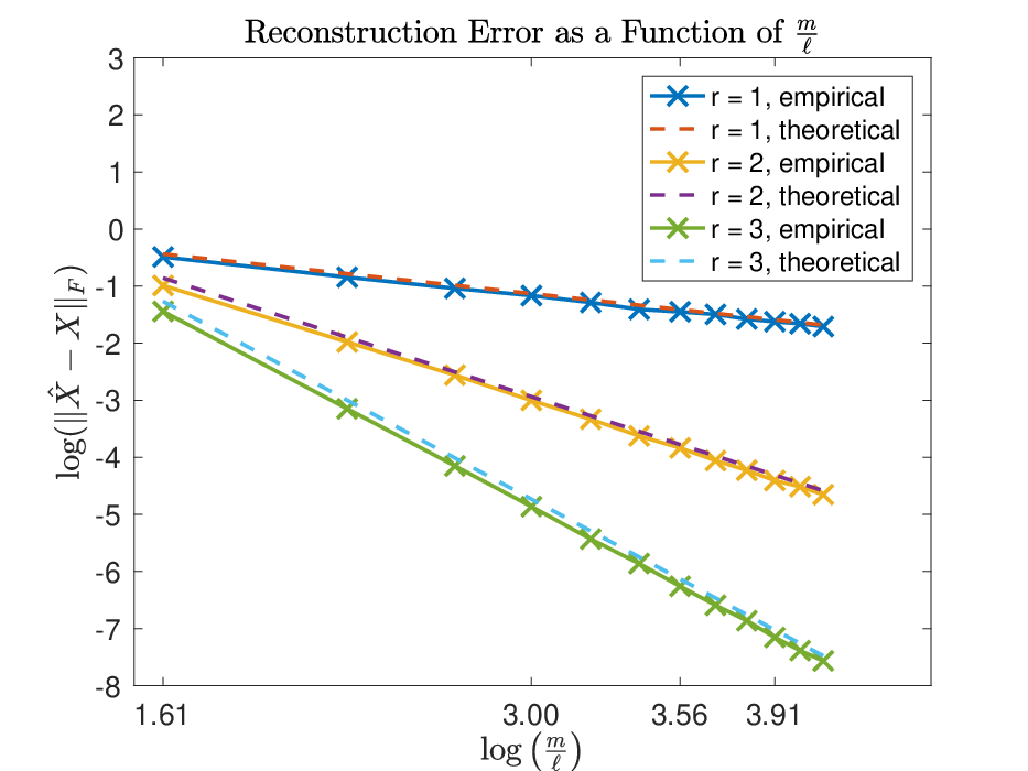
First, we illustrate the decay of the reconstruction error, measured in the Frobenius norm, as a function of the order of the quantization scheme for , and in the noise-less setting. Experiments were run with the following parameters: , , alphabet step-size , rank , and . We let the over-sampling factor range from to by a step size of . The reconstruction error for a fixed over-sampling factor was averaged over 20 draws of . The results are reported in Figure 2 for the three choices of . As Theorem 12 predicts, the reconstruction error decays polynomially in the oversampling rate, with the polynomial degree increasing with .

To test the dependence on measurement noise, we considered reconstructing matrices from measurements generated by a fixed draw of . For , we averaged our reconstruction error over 20 trials with noise vectors drawn from the uniform distribution on and normalized to have . The remaining parameters were set to the following values: , alphabet step-size , rank , , and . Figure 2 illustrates the outcome of this experiment, which agrees with the bound in Theorem 12.
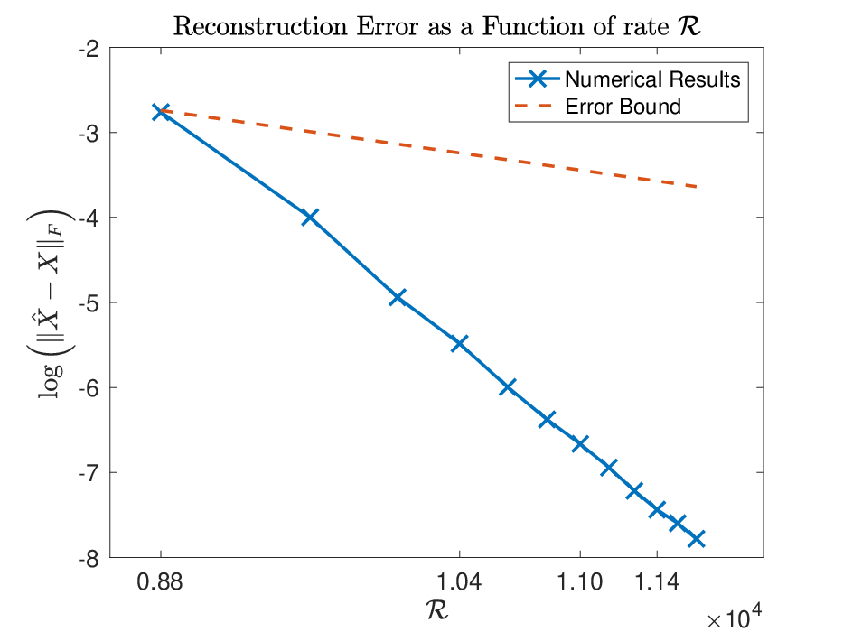
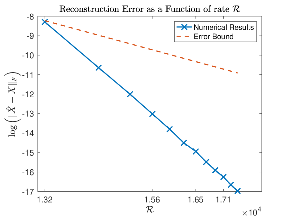
The goal of the next experiment is to illustrate, in the context of encoding (Corollary 14), the exponential decay of distortion as a function of the rate, or equivalently of the reconstruction error as a function of the number of bits (i.e., rate) used. We performed numerical simulations for schemes of order 2 and 3. As before, our parameters were set to the following: , , rank of the true matrix , , , and let range from to by a step size of . The rate is calculated to be . Again, the reconstruction error for a fixed over-sampling factor was averaged over 20 draws of . The results are shown in Figures 4 and 4, respectively. The slopes of the lines (corresponding to the constant in the exponent in the rate-distortion relationship) which pass through the first and last points of each plot are and for , respectively. It should further be noted that the numerical distortions decay much faster than the upper bound of (28). We suspect this to be due to the sub-optimal -dependent constants in the exponent of (28), which are likely an artifact of the proof technique in [35]. Indeed, there is evidence in [35] that the correct exponent is rather than . This is more in line with our numerical exerpiments but the proof of such is beyond the scope of this paper.
Acknowledgements
RS was supported in part by the NSF via DMS-1517204. Additionally, both authors acknowledge support from a UCSD senate research grant award.
References
- [1] John J Benedetto, O Yilmaz, and Alexander M Powell. Sigma-delta quantization and finite frames. In Acoustics, Speech, and Signal Processing, 2004. Proceedings.(ICASSP’04). IEEE International Conference on, volume 3, pages iii–937. IEEE, 2004.
- [2] Sonia A Bhaskar and Adel Javanmard. 1-bit matrix completion under exact low-rank constraint. In Information Sciences and Systems (CISS), 2015 49th Annual Conference on, pages 1–6. IEEE, 2015.
- [3] Petros T Boufounos, Laurent Jacques, Felix Krahmer, and Rayan Saab. Quantization and compressive sensing. In Compressed Sensing and its Applications, pages 193–237. Springer, 2015.
- [4] Tony Cai and Wen-Xin Zhou. A max-norm constrained minimization approach to 1-bit matrix completion. The Journal of Machine Learning Research, 14(1):3619–3647, 2013.
- [5] E. J. Candès, J. Romberg, and T. Tao. Stable signal recovery from incomplete and inaccurate measurements. Comm. Pure Appl. Math., 59:1207–1223, 2006.
- [6] Emmanuel J Candès, Xiaodong Li, Yi Ma, and John Wright. Robust principal component analysis? Journal of the ACM (JACM), 58(3):11, 2011.
- [7] Emmanuel J Candes and Yaniv Plan. Tight oracle inequalities for low-rank matrix recovery from a minimal number of noisy random measurements. Information Theory, IEEE Transactions on, 57(4):2342–2359, 2011.
- [8] Emmanuel J Candès and Benjamin Recht. Exact matrix completion via convex optimization. Foundations of Computational mathematics, 9(6):717, 2009.
- [9] Emmanuel J Candès and Terence Tao. The power of convex relaxation: Near-optimal matrix completion. IEEE Transactions on Information Theory, 56(5):2053–2080, 2010.
- [10] I. Daubechies and R. DeVore. Approximating a bandlimited function using very coarsely quantized data: a family of stable sigma-delta modulators of arbitrary order. Ann. Math., 158(2):679–710, 2003.
- [11] Mark A Davenport, Yaniv Plan, Ewout Van Den Berg, and Mary Wootters. 1-bit matrix completion. Information and Inference: A Journal of the IMA, 3(3):189–223, 2014.
- [12] P. Deift, C. S. Güntürk, and F. Krahmer. An optimal family of exponentially accurate one-bit sigma-delta quantization schemes. Comm. Pure Appl. Math., 64(7):883–919, 2011.
- [13] Richard M Dudley. The sizes of compact subsets of hilbert space and continuity of gaussian processes. Journal of Functional Analysis, 1(3):290–330, 1967.
- [14] Maryam Fazel. Matrix rank minimization with applications. PhD thesis, PhD thesis, Stanford University, 2002.
- [15] Joe-Mei Feng, Felix Krahmer, and Rayan Saab. Quantized compressed sensing for partial random circulant matrices. arXiv preprint arXiv:1702.04711, 2017.
- [16] Simon Foucart and Holger Rauhut. A mathematical introduction to compressive sensing. Birkhäuser Basel, 2013.
- [17] D. Gross, Y.-K. Liu, S. T. Flammia, S. Becker, and J. Eisert. Quantum State Tomography via Compressed Sensing. Physical Review Letters, 105(15):150401, October 2010.
- [18] C Sinan Güntürk, Mark Lammers, Alex Powell, Rayan Saab, and Özgür Yilmaz. Sigma delta quantization for compressed sensing. In Information Sciences and Systems (CISS), 2010 44th Annual Conference on, pages 1–6. IEEE, 2010.
- [19] C.S. Güntürk. One-bit sigma-delta quantization with exponential accuracy. Comm. Pure Appl. Math., 56(11):1608–1630, 2003.
- [20] H. Inose and Y. Yasuda. A unity bit coding method by negative feedback. Proceedings of the IEEE, 51(11):1524–1535, 1963.
- [21] Mark Iwen and Rayan Saab. Near-optimal encoding for sigma-delta quantization of finite frame expansions. Journal of Fourier Analysis and Applications, 19(6):1255–1273, 2013.
- [22] William B Johnson and Joram Lindenstrauss. Extensions of lipschitz mappings into a hilbert space. Contemporary mathematics, 26(189-206):1, 1984.
- [23] Raghunandan H Keshavan, Andrea Montanari, and Sewoong Oh. Matrix completion from noisy entries. Journal of Machine Learning Research, 11(Jul):2057–2078, 2010.
- [24] Felix Krahmer, Shahar Mendelson, and Holger Rauhut. Suprema of chaos processes and the restricted isometry property. Communications on Pure and Applied Mathematics, 67(11):1877–1904, 2014.
- [25] Felix Krahmer, Rayan Saab, and Rachel Ward. Root-exponential accuracy for coarse quantization of finite frame expansions. IEEE Transactions on Information Theory, 58(2):1069–1079, 2012.
- [26] Felix Krahmer, Rayan Saab, and Özgür Yilmaz. Sigma–delta quantization of sub-gaussian frame expansions and its application to compressed sensing. Information and Inference: A Journal of the IMA, 3(1):40–58, 2014.
- [27] Jean Lafond, Olga Klopp, Eric Moulines, and Joseph Salmon. Probabilistic low-rank matrix completion on finite alphabets. In Advances in Neural Information Processing Systems, pages 1727–1735, 2014.
- [28] Andrew S Lan, Christoph Studer, and Richard G Baraniuk. Matrix recovery from quantized and corrupted measurements. In Acoustics, Speech and Signal Processing (ICASSP), 2014 IEEE International Conference on, pages 4973–4977. IEEE, 2014.
- [29] Zhouchen Lin, Minming Chen, and Yi Ma. The augmented lagrange multiplier method for exact recovery of corrupted low-rank matrices. arXiv preprint arXiv:1009.5055, 2010.
- [30] Samet Oymak, Karthik Mohan, Maryam Fazel, and Babak Hassibi. A simplified approach to recovery conditions for low rank matrices. In Information Theory Proceedings (ISIT), 2011 IEEE International Symposium on, pages 2318–2322. IEEE, 2011.
- [31] Rong Pan, Yunhong Zhou, Bin Cao, Nathan N Liu, Rajan Lukose, Martin Scholz, and Qiang Yang. One-class collaborative filtering. In Data Mining, 2008. ICDM’08. Eighth IEEE International Conference on, pages 502–511. IEEE, 2008.
- [32] Swati Rallapalli, Lili Qiu, Yin Zhang, and Yi-Chao Chen. Exploiting temporal stability and low-rank structure for localization in mobile networks. In Proceedings of the sixteenth annual international conference on Mobile computing and networking, pages 161–172. ACM, 2010.
- [33] Benjamin Recht, Maryam Fazel, and Pablo A Parrilo. Guaranteed minimum-rank solutions of linear matrix equations via nuclear norm minimization. SIAM review, 52(3):471–501, 2010.
- [34] Rayan Saab, Rongrong Wang, and Özgür Yılmaz. Quantization of compressive samples with stable and robust recovery. Applied and Computational Harmonic Analysis, 2016.
- [35] Rayan Saab, Rongrong Wang, and Özgür Yılmaz. From compressed sensing to compressed bit-streams: practical encoders, tractable decoders. IEEE Transactions on Information Theory, 2017.
- [36] M. Talagrand. The Generic Chaining. Springer-Verlag, 2005.
- [37] Roman Vershynin. Introduction to the non-asymptotic analysis of random matrices, pages 210 – 268. Cambridge University Press, 2012.