跳到论文正文
W Papers独立论文阅读器 arXiv:1709.09565 论文正文 计算阅读时间 · 0%
引用这篇论文根据当前论文元数据生成,正式投稿前建议核对。


License: arXiv.org perpetual non-exclusive license
arXiv:1709.09565v2 [math.ST] 02 May 2019

Entrywise Eigenvector Analysis of Random Matrices with Low Expected Rank

Emmanuel Abbe ††thanks: Address: PACM and Department of EE, Princeton University, Princeton, NJ 08544, USA; E-mail: eabbe@princeton.edu. The research was supported by NSF CAREER Award CCF-1552131, ARO grant W911NF-16-1-0051, NSF CSOI CCF-0939370.    Jianqing Fan ††thanks: Address: Department of ORFE, Sherrerd Hall, Princeton University, Princeton, NJ 08544, USA; E-mails: {jqfan, kaizheng, yiqiaoz}@princeton.edu. The research was supported by NSF grants DMS-1662139 and DMS-1712591, NIH grant R01-GM072611-11 and ONR grant N00014-19-1-2120.    Kaizheng Wang    Yiqiao Zhong
Abstract

Recovering low-rank structures via eigenvector perturbation analysis is a common problem in statistical machine learning, such as in factor analysis, community detection, ranking, matrix completion, among others. While a large variety of bounds are available for average errors between empirical and population statistics of eigenvectors, few results are tight for entrywise analyses, which are critical for a number of problems such as community detection.

This paper investigates entrywise behaviors of eigenvectors for a large class of random matrices whose expectations are low-rank, which helps settle the conjecture in Abbe et al. (2014b) that the spectral algorithm achieves exact recovery in the stochastic block model without any trimming or cleaning steps. The key is a first-order approximation of eigenvectors under the ℓ∞\ell_{\infty} norm:

uk≈A​uk∗λk∗,u_{k}\approx\frac{Au_{k}^{*}}{\lambda_{k}^{*}},

where {uk}\{u_{k}\} and {uk∗}\{u_{k}^{*}\} are eigenvectors of a random matrix AA and its expectation 𝔼​A\mathbb{E}A, respectively. The fact that the approximation is both tight and linear in AA facilitates sharp comparisons between uku_{k} and uk∗u_{k}^{*}. In particular, it allows for comparing the signs of uku_{k} and uk∗u_{k}^{*} even if ‖uk−uk∗‖∞\|u_{k}-u_{k}^{*}\|_{\infty} is large. The results are further extended to perturbations of eigenspaces, yielding new ℓ∞\ell_{\infty}-type bounds for synchronization (ℤ2\mathbb{Z}_{2}-spiked Wigner model) and noisy matrix completion.

Keywords: Eigenvector perturbation, spectral analysis, synchronization, community detection, matrix completion, low-rank structures, random matrices.

1 Introduction

Many estimation problems in statistics involve low-rank matrix estimators that are NP-hard to compute, and many of these estimators are solutions to nonconvex programs. This is partly because of the widespread use of maximum likelihood estimation (MLE) which, while enjoying good statistical properties, often poses computational challenges due to nonconvex or discrete constraints inherent in the problems.

Fortunately, computationally efficient algorithms using eigenvectors often afford good performance. The eigenvectors either directly lead to final estimates (Shi and Malik, 2000; Ng et al., 2002), or serve as warm starts followed by further refinements (Keshavan et al., 2010a; Jain et al., 2013; Candès et al., 2015). Such algorithms mostly rely on computation of leading eigenvectors and matrix-vector multiplications, which are easily implemented.

While various heuristics abound, theoretical understanding remains scarce on the entrywise analysis, and on when refinements are needed or can be avoided. In particular, it remains open in various cases to determine whether a vanilla eigenvector-based method without preprocessing steps (e.g., trimming of outliers) or without refinement steps (e.g., cleaning with local improvements) enjoys the same optimality results as the MLE (or SDP) does. A crucial missing step is a sharp entrywise perturbation analysis of eigenvectors. This is party because the ℓ∞\ell_{\infty} distance between the eigenvectors of a random matrix and their expected counterparts may not be the correct quantity to look at; errors per entry can be asymmetrically distributed, as we shall see in this paper.

This paper investigates entrywise behaviors of eigenvectors and more generally, eigenspaces, for random matrices with low expected rank using the following approach. Let AA be a random matrix, A∗=𝔼​AA^{*}=\mathbb{E}A, and E=A−A∗E=A-A^{*} be the ‘error’ of AA. In many cases, A∗A^{*} is a symmetric matrix with low rank determined by the structure of a statistical problem, such as low-rank with blocks in community detection.

Consider for now the case of symmetric AA, and let uku_{k}, resp. uk∗u_{k}^{*}, be the eigenvector corresponding to the kk-th largest eigenvalue of AA, resp. A∗A^{*}. Roughly speaking, if EE is moderate, our first-order approximation reads

uk=A​ukλk≈A​uk∗λk∗=uk∗+E​uk∗λk∗.u_{k}=\frac{Au_{k}}{\lambda_{k}}\approx\frac{Au_{k}^{*}}{\lambda_{k}^{*}}=u_{k}^{*}+\frac{Eu_{k}^{*}}{\lambda_{k}^{*}}.

While uku_{k} is a nonlinear function of AA (or equivalently EE), the approximation is linear in AA, which greatly facilitates the analysis. Under certain conditions, the maximum entrywise approximation error ‖uk−A​uk∗/λk∗‖∞\|u_{k}-Au_{k}^{*}/\lambda_{k}^{*}\|_{\infty} can be much smaller than ‖uk∗‖∞\|u^{*}_{k}\|_{\infty}, allowing us to study uku_{k} through A​uk∗/λk∗Au_{k}^{*}/\lambda_{k}^{*}. To obtain such results, a key part in our theory is to characterize concentration properties of AA and structural assumptions on its expectation A∗A^{*}.

This perturbation analysis leads to new and sharp theoretical guarantees. In particular, we find that for the exact recovery problem in stochastic block model, the vanilla spectral algorithm (without trimming or cleaning) achieves the information-theoretic limit, and it coincides with the MLE estimator whenever the latter succeeds. This settles in particular a conjecture left open in Abbe et al. (2014b); Abbe et al. (2016). Therefore, MLE and SDP do not have advantage over the spectral method in terms of exact recovery, if the model is correct. SDP may be preferred in some applications for its robustness and optimality certificates, but that is beyond the scope of this paper.

1.1 A sample problem

Let us consider a network model that has received widespread interest in recent years: the stochastic block model (SBM). Suppose that we have a graph with vertex set {1,2,⋯,n}\{1,2,\cdots,n\}, and assume for simplicity that nn is even. There is an unknown index set J∈{1,2,⋯,n}J\in\{1,2,\cdots,n\} with |J|=n/2|J|=n/2 such that the vertex set is partitioned into two groups JJ and JcJ^{c}. Within groups, there is an edge between each pair of vertices with probability pp, and between groups, there is an edge with probability qq. Let x∈ℝnx\in\mathbb{R}^{n} be the group membership vector with xi=1x_{i}=1 if i∈Ji\in J and xi=−1x_{i}=-1 otherwise. The goal is to recover xx from the observed edges of the graph.

This random-graph-based model was first proposed for social relationship networks (Holland et al., 1983), and many more realistic models have been developed based on the SBM since then. Given its fundamental importance, there are a plurality of papers addressing statistical properties and algorithmic efficiencies; see Abbe (2017) for a survey.

Under the regime p=a​log⁡nnp=\frac{a\log n}{n}, q=b​log⁡nnq=\frac{b\log n}{n} where a>b>0a>b>0 are constants, Abbe et al. (2016) and Mossel et al. (2014) proved that exact recovery is possible if and only if a−b>2\sqrt{a}-\sqrt{b}>\sqrt{2}, and that the limit can be achieved by efficient algorithms. They used two-round procedures (with a clean-up phase) to achieve the threshold. Semidefinite relaxations are also known to achieve the threshold (Abbe et al., 2016; Hajek et al., 2016; Agarwal et al., 2015; Bandeira, 2015), as well as spectral methods with local refinements (Abbe and Sandon, 2015; Yun and Proutiere, 2016; Gao et al., 2015). We will discuss more in Sections 1.5 and 3.2.

While existing works tackle exact recovery rather successfully, some fundamental questions remain unsolved: how do the simple statistics—top eigenvectors of the adjacency matrix—behave? Are they informative enough to reveal the group structure under very challenging regimes?

Figure 1: The second eigenvector and its first-order approximation in SBM. Left: The histogram of coordinates of n​u2\sqrt{n}\,u_{2} computed from a single realization of adjacency matrix AA, where nn is 50005000, aa is 4.54.5 and bb is 0.250.25. Exact recovery is expected as coordinates form two well-separated clusters. Right: boxplots showing three different distance/errors (up to sign) over 100100 realizations: (i) n​‖u2−u2∗‖∞\sqrt{n}\,\|u_{2}-u_{2}^{*}\|_{\infty}, (ii) n​‖A​u2∗/λ2∗−u2∗‖∞\sqrt{n}\,\|Au_{2}^{*}/\lambda_{2}^{*}-u_{2}^{*}\|_{\infty}, (iii) n​‖u2−A​u2∗/λ2∗‖∞\sqrt{n}\,\|u_{2}-Au_{2}^{*}/\lambda_{2}^{*}\|_{\infty}. A​u2∗/λ2∗Au_{2}^{*}/\lambda_{2}^{*} is a good approximation of u2u_{2} under ℓ∞\ell_{\infty} norm even though ‖u2−u2∗‖∞\|u_{2}-u_{2}^{*}\|_{\infty} may be large.

To study these questions, we start with the eigenvectors of A∗=𝔼​AA^{*}=\mathbb{E}A. By definition, Ai​jA_{ij} is a Bernoulli random variable, and ℙ⁡(Ai​j=1)\mathbb{P}(A_{ij}=1) depends on whenever ii and jj are from the same groups. The expectation 𝔼​A\mathbb{E}A must be a block matrix of the following form:

𝔼​A=log⁡nn​(a​𝟏n2×n2b​𝟏n2×n2b​𝟏n2×n2a​𝟏n2×n2),\mathbb{E}A=\frac{\log n}{n}\left(\begin{array}[]{cc}a\mathbf{1}_{\frac{n}{2}\times\frac{n}{2}}&b\mathbf{1}_{\frac{n}{2}\times\frac{n}{2}}\\ b\mathbf{1}_{\frac{n}{2}\times\frac{n}{2}}&a\mathbf{1}_{\frac{n}{2}\times\frac{n}{2}}\end{array}\right),

where 𝟏m×m\mathbf{1}_{m\times m} is the m×mm\times m all-one matrix. Here, for convenience, we represent 𝔼​A\mathbb{E}A as if J={1,2,⋯,n/2}J=\{1,2,\cdots,n/2\}. But in general JJ is unknown, and there is a permutation of indices {1,⋯,n}\{1,\cdots,n\} in the matrix representation.

From the matrix representation it is clear that 𝔼​A\mathbb{E}A has rank 22, with two nonzero eigenvalues λ1∗=a+b2​log⁡n\lambda_{1}^{*}=\frac{a+b}{2}\log n and λ2∗=a−b2​log⁡n\lambda_{2}^{*}=\frac{a-b}{2}\log n. Simple calculations give the corresponding (normalized) eigenvectors: u1∗=1n​𝟏nu_{1}^{*}=\frac{1}{\sqrt{n}}\mathbf{1}_{n}, and (u2∗)i=1/n(u_{2}^{*})_{i}=1/\sqrt{n} if i∈Ji\in J and (u2∗)i=−1/n(u_{2}^{*})_{i}=-1/\sqrt{n} if i∈Jci\in J^{c}. Since u2∗u_{2}^{*} perfectly aligns with the group assignment vector xx, we hope to show its counterpart u2u_{2}, i.e., the second eigenvector of AA, also has desirable properties.

The first reassuring fact is that, the top eigenvalues preserve proper ordering: by Weyl’s inequality, the deviation of any eigenvalue λi\lambda_{i} (i∈[n]i\in[n]) from λi∗\lambda_{i}^{*} is bounded by ‖A−A∗‖2\|A-A^{*}\|_{2}, which is O⁡(log⁡n)O(\sqrt{\log n}) with high probability; see supplementary materials (Abbe et al., 2018). The Davis-Kahan sin⁡Θ\sin\Theta theorem asserts that u1u_{1} and u2u_{2} are weakly consistent estimators for u1∗u_{1}^{*} and u2∗u_{2}^{*} respectively, in the sense that |⟨uk,uk∗⟩|→ℙ1|\langle u_{k},u_{k}^{*}\rangle|\xrightarrow{\mathbb{P}}1 for k=1,2k=1,2. However, this is not helpful for understanding their entrywise behaviors in the uniform sense, which is crucial for exact recovery. Nor can it explain the sharp phase transition phenomenon. This makes entrywise analysis both interesting and challenging.

This problem motivates some simulations about the coordinates of top eigenvectors of AA. In Figure 1, we calculate the rescaled second eigenvector n​u2\sqrt{n}u_{2} of one typical realization AA, and make a histogram plot of its coordinates. (Note the first eigenvector is aligned with the all-one vector 𝟏n\mathbf{1}_{n}, which is uninformative.) The parameters we choose are n=5000n=5000, a=4.5a=4.5 and b=0.25b=0.25, for which exact recovery is possible with high probability. Visibly, the coordinates of n​u2\sqrt{n}u_{2} form two clusters around ±1\pm 1 which, marked by red dashed lines, are coordinates of n​u2∗\sqrt{n}\,u_{2}^{*}. Intuitively, the signs of the former should suffice to reveal the group structure.

To probe into the second eigenvector u2u_{2}, we expand the perturbation u2−u2∗u_{2}-u_{2}^{*} as follows:

u2−u2∗=(A​u2∗λ2∗−u2∗)+(u2−A​u2∗λ2∗).u_{2}-u_{2}^{*}=\left(\frac{Au_{2}^{*}}{\lambda_{2}^{*}}-u_{2}^{*}\right)+\left(u_{2}-\frac{Au_{2}^{*}}{\lambda_{2}^{*}}\right). (1.1)

The first term is exactly E​u2∗/λ2∗Eu_{2}^{*}/\lambda_{2}^{*}, which is linear in EE and can be viewed as the first-order perturbation. The second term is nonlinear in general, representing the error of higher order. Figure 1 shows boxplots of the infinity norm of rescaled perturbation errors over 100100 realizations (see (i)-(iii)), which illustrates that ‖u2−A​u2∗/λ2∗‖∞\|u_{2}-Au_{2}^{*}/\lambda_{2}^{*}\|_{\infty} is much smaller than ‖u2−u2∗‖∞\|u_{2}-u_{2}^{*}\|_{\infty} and ‖A​u2∗/λ2∗−u2∗‖∞\|Au_{2}^{*}/\lambda_{2}^{*}-u_{2}^{*}\|_{\infty}. Indeed, we will see in Theorem 1.1 that

‖u2−A​u2∗/λ2∗‖∞=oℙ​(mini⁡|(u2∗)i|)=oℙ​(1/n).\left\|u_{2}-Au_{2}^{*}/\lambda_{2}^{*}\right\|_{\infty}=o_{\mathbb{P}}\left(\min_{i}|(u_{2}^{*})_{i}|\right)=o_{\mathbb{P}}\left(1/\sqrt{n}\right). (1.2)

The result holds ‘up to sign’, i.e. can choose an appropriate sign for the eigenvector u2u_{2} as it is not uniquely defined; see Theorem 1.1 for its precise meaning. Therefore, the entrywise behavior of u2−u2∗u_{2}-u_{2}^{*} is captured by its first-order term, which is much more amenable to analysis. This observation will finally lead to sharp eigenvector results in Section 3.2.

We remark that it is also possible to study the top eigenvector (denoted as u¯\bar{u}) of the centered adjacency matrix A¯=A−d^n​𝟏n​𝟏nT\bar{A}=A-\frac{\hat{d}}{n}\mathbf{1}_{n}\mathbf{1}_{n}^{T}, where d^=∑i,jAi​j/n\hat{d}=\sum_{i,j}A_{ij}/n is the average degree of all vertices. The top eigenvector of 𝔼​A¯\mathbb{E}\bar{A} is exactly u2∗u_{2}^{*}, and its empirical counterpart u¯\bar{u} is very similar to u2u_{2}. In fact, the same reasoning and analysis applies to u¯\bar{u}, and one obtains similar plots as Figure 1 (omitted here).

1.2 First-order approximation of eigenvectors

Now we present a simpler version of our result that justifies the intuitions above. Consider a general symmetric random matrix (more precisely, this should be a sequence of random matrices with growing dimensions) A∈ℝn×nA\in\mathbb{R}^{n\times n} with independent entries on and above its diagonal. Suppose its expectation A∗=𝔼​A∈ℝn×nA^{*}=\mathbb{E}A\in\mathbb{R}^{n\times n} is low-rank and has rr nonzero eigenvalues. Let us assume that

  • (a) r=O⁡(1)r=O(1), these rr eigenvalues are positive and in descending order (λ1∗≥λ2∗≥⋯≥λr∗>0\lambda_{1}^{*}\geq\lambda_{2}^{*}\geq\cdots\geq\lambda_{r}^{*}>0), and λ1∗≍λr∗\lambda_{1}^{*}\asymp\lambda_{r}^{*}.

Their corresponding eigenvectors are denoted by u1∗,⋯,ur∗∈ℝnu_{1}^{*},\cdots,u_{r}^{*}\in\mathbb{R}^{n}. In other words, we have spectral decomposition A∗=∑j=1rλj∗​uj∗​(uj∗)TA^{*}=\sum_{j=1}^{r}\lambda_{j}^{*}u_{j}^{*}(u_{j}^{*})^{T}.

We fix k∈[r]k\in[r] and study the kk-th eigenvector uku_{k}. Define the eigen-gap (or spectral gap) as Δ∗=min⁡{λk−1∗−λk∗,λk∗−λk+1∗}\Delta^{*}=\min\{\lambda_{k-1}^{*}-\lambda_{k}^{*},\lambda_{k}^{*}-\lambda_{k+1}^{*}\}, where we adopt the convention λ0∗=+∞\lambda_{0}^{*}=+\infty and λn+1∗=−∞\lambda_{n+1}^{*}=-\infty. Assume that

  • (b) AA concentrates under the spectral norm, i.e., there is a suitable γ=γn=o⁡(1)\gamma=\gamma_{n}=o(1) such that ‖A−A∗‖2≤γ​Δ∗\|A-A^{*}\|_{2}\leq\gamma\Delta^{*} holds with probability 1−o⁡(1)1-o(1).

A direct yet important implication is that, the fluctuation of λk\lambda_{k} is much smaller than the gap Δ∗\Delta^{*}, since Weyl’s inequality forces |λk−λk∗|≤‖A−A∗‖2|\lambda_{k}-\lambda_{k}^{*}|\leq\|A-A^{*}\|_{2}. Thus, λk\lambda_{k} is well separated from other eigenvalues, including the ‘bulk’ n−rn-r eigenvalues whose magnitudes are at most ‖E‖2\|E\|_{2}.

In addition, we assume that AA concentrates in a row-wise sense:

  • (c) there exists a continuous non-decreasing function φ:ℝ+→ℝ+\varphi:\mathbb{R}_{+}\to\mathbb{R}_{+} that possibly depends on nn, such that φ⁡(0)=0\varphi(0)=0, φ⁡(x)/x\varphi(x)/x is non-increasing, and that for any m∈[n],w∈ℝnm\in[n],w\in\mathbb{R}^{n}, with probability 1−o⁡(n−1)1-o(n^{-1}),

    |(A−A∗)m⋅w|≤Δ∗∥w∥∞φ(‖w‖2n​‖w‖∞).|(A-A^{*})_{m\cdot}w|\leq\Delta^{*}\|w\|_{\infty}\,\varphi\Big(\frac{\|w\|_{2}}{\sqrt{n}\|w\|_{\infty}}\Big).

Here, the notation (A−A∗)m⋅(A-A^{*})_{m\cdot} means the mm-th row vector of A−A∗A-A^{*}.

For the Gaussian case where Ai​j∼N⁡(Ai​j∗,σ2)A_{ij}\sim N(A_{ij}^{*},\sigma^{2}), we can simply choose a linear function φ⁡(x)=c​(Δ∗)−1​σ​n​log⁡n​x\varphi(x)=c(\Delta^{*})^{-1}\sigma\sqrt{n\log n}\,x where c>0c>0 is some proper constant. The condition then reads

ℙ(|(A−A∗)m⋅w|≤cσlog⁡n∥w∥2)=1−o(n−1),\mathbb{P}\left(|(A-A^{*})_{m\cdot}w|\leq c\sigma\sqrt{\log n}\|w\|_{2}\right)=1-o(n^{-1}),

which directly follows from Gaussian tail bound since (A−A∗)m⋅w∼N(0,σ2∥w∥22)(A-A^{*})_{m\cdot}w\sim N(0,\sigma^{2}\|w\|_{2}^{2}). The tail of (A−A∗)m⋅w(A-A^{*})_{m\cdot}w is completely determined by ‖w‖2\|w\|_{2}. For Bernoulli variables, we will use Bernstein-type inequalities to study (A−A∗)m⋅w(A-A^{*})_{m\cdot}w, which will inevitably involve both ‖w‖2\|w\|_{2} and ‖w‖∞\|w\|_{\infty}. Hence the function φ⁡(x)\varphi(x) can no longer be linear. It turns out that φ⁡(x)∝(1∨log⁡(1/x))−1\varphi(x)\propto(1\vee\log(1/x))^{-1}, shown in Figure 2, is a suitable choice. More details can be found in Section 2.1 and the supplementary material Abbe et al. (2018). In both cases we have φ⁡(1)=O⁡(1)\varphi(1)=O(1) under suitable signal-to-noise conditions.

xxφ⁡(x)\varphi(x)GaussianBernoulli
Figure 2: Typical choices of φ\varphi for Gaussian noise and Bernoulli noise.
Theorem 1.1 (Simpler form of Theorem 2.1).

Let k∈[r]={1,2,⋯,r}k\in[r]=\{1,2,\cdots,r\} be fixed. Suppose that Assumptions (a), (b) and (c) hold, and ‖uk∗‖∞≤γ\|u_{k}^{*}\|_{\infty}\leq\gamma. Then, with probability 1−o⁡(1)1-o(1),

mins∈{±1}⁡‖uk−s​A​uk∗/λk∗‖∞=O⁡((γ+φ⁡(γ))​‖uk∗‖∞)=o⁡(‖uk∗‖∞),\min_{s\in\{\pm 1\}}\|u_{k}-sAu_{k}^{*}/\lambda_{k}^{*}\|_{\infty}=O\big((\gamma+\varphi(\gamma))\|u_{k}^{*}\|_{\infty}\big)=o\big(\|u_{k}^{*}\|_{\infty}\big), (1.3)

where the notations O⁡(⋅)O(\cdot) and o⁡(⋅)o(\cdot) hide dependencies on φ⁡(1)\varphi(1).

On the left-hand side, we are allowed to choose a suitable sign ss as eigenvectors are not uniquely defined. The second bound is a consequence of the first one, since γ=o⁡(1)\gamma=o(1) and limγ→0φ⁡(γ)=0\lim_{\gamma\to 0}\varphi(\gamma)=0 by continuity. We hide dependency on φ⁡(1)\varphi(1) in the above bound, since φ⁡(1)\varphi(1) is bounded by a constant under suitable signal-to-noise ratio. More details can be found in Theorem 2.1. Therefore, the approximation error ‖uk−A​uk∗/λk∗‖∞\|u_{k}-Au_{k}^{*}/\lambda_{k}^{*}\|_{\infty} is much smaller than ‖uk∗‖∞\|u_{k}^{*}\|_{\infty}. This rigorously confirms the intuitions in Section 1.1.

Here are some remarks. (1) This theorem enables us to study uku_{k} via its linearization A​uk∗/λk∗Au_{k}^{*}/\lambda_{k}^{*}, since the approximation error is usually small order-wise. (2) The conditions of the theorem are fairly mild. For SBM, the theorem is applicable as long as we are in the log⁡nn\frac{\log n}{n} regime (p=a​log⁡nnp=a\frac{\log n}{n} and q=b​log⁡nnq=b\frac{\log n}{n}), regardless of the relative sizes of aa and bb.

1.3 MLE, spectral algorithm, and strong consistency

Once we obtain the approximation result (1.3), the analysis of entrywise behavior of eigenvectors boils down to that of A​uk∗/λk∗Au_{k}^{*}/\lambda_{k}^{*}. In the SBM example, suppose we have (1.2) and with probability 1−o⁡(1)1-o(1), sgn⁡(A​u2∗/λ2∗)=sgn⁡(u2∗)\mathrm{sgn}(Au_{2}^{*}/\lambda_{2}^{*})=\mathrm{sgn}(u_{2}^{*}) and all the entries of A​u2∗/λ2∗Au_{2}^{*}/\lambda_{2}^{*} are bounded away from zero by an order of 1/n1/\sqrt{n}. Then sgn⁡(u2)=sgn⁡(A​u2∗/λ2∗)\mathrm{sgn}(u_{2})=\mathrm{sgn}(Au_{2}^{*}/\lambda_{2}^{*}) holds with probability 1−o⁡(1)1-o(1). Here sgn⁡(⋅)\mathrm{sgn}(\cdot) denotes the entrywise sign function. The eigenvector-based estimator sgn⁡(u2)\mathrm{sgn}(u_{2}) for block membership can be conveniently analyzed through A​u2∗/λ2∗Au_{2}^{*}/\lambda_{2}^{*}, whose entries are just linear combinations of Bernoulli variables.

We remark on a subtlety of our result: our central analysis is a good control of ‖uk−A​uk∗/λk∗‖∞\|u_{k}-Au_{k}^{*}/\lambda_{k}^{*}\|_{\infty}, not necessarily of ‖uk−uk∗‖∞\|u_{k}-u_{k}^{*}\|_{\infty}. For example, in SBM, an inequality such as ‖u2−u2∗‖∞<‖u2∗‖∞\|u_{2}-u_{2}^{*}\|_{\infty}<\|u_{2}^{*}\|_{\infty} is not true in general. In Figure 1, the second boxplot shows that n​‖u2−u2∗‖∞\sqrt{n}\,\|u_{2}-u_{2}^{*}\|_{\infty} may well exceed 11 even if sgn⁡(u2)=sgn⁡(u2∗)\mathrm{sgn}(u_{2})=\mathrm{sgn}(u_{2}^{*}). This suggests that the distributions of the coordinates of the two clusters, though well separated, have asymmetric tails. Our Theorem 3.3 asserts that it is in vain to seek a good bound for ‖u2−u2∗‖∞\|u_{2}-u_{2}^{*}\|_{\infty}. Instead, one should resort to the central quantity A​u2∗/λ2∗Au_{2}^{*}/\lambda_{2}^{*}. This may partly explain why the conjecture has remained open for long.

The vector A​uk∗/λk∗Au_{k}^{*}/\lambda_{k}^{*} also plays a pivotal role in the information-theoretic lower bound for exact recovery in SBM, established in Abbe et al. (2016). It is necessary to ensure (A​u2∗/λ2∗)i>0,∀i∈J(Au_{2}^{*}/\lambda_{2}^{*})_{i}>0,\forall i\in J to hold with probability at least 1/31/3. Otherwise, by symmetry and the union bound, with probability at least 1/31/3 we can find some i∈Ji\in J and i′∈Jci^{\prime}\in J^{c} with (A​u2∗/λ2∗)i<0(Au_{2}^{*}/\lambda_{2}^{*})_{i}<0 and (A​u2∗/λ2∗)i′>0(Au_{2}^{*}/\lambda_{2}^{*})_{i^{\prime}}>0. Elementary calculation shows that in that case, a swap of group assignments of ii and i′i^{\prime} increases the likelihood. Thus the MLE x^MLE\hat{x}_{\mbox{\scriptsize MLE}} fails to exactly recover JJ. With a uniform prior on group assignments, the MLE is equivalent to the maximum a posteriori estimator, which is optimal for exact recovery. Therefore, we must eliminate such local refinements to make exact recovery possible. This forms the core argument in Abbe et al. (2016). The analysis above suggests an interesting property about the eigenvector-based estimator x^e​i​g​(A):=sgn⁡(u2)\hat{x}_{eig}(A):=\mathrm{sgn}(u_{2}):

Corollary 1.1.

Suppose we are given a>b>0a>b>0 such that a≠b+2\sqrt{a}\neq\sqrt{b}+\sqrt{2}, i.e., we exclude the regime where (a,b)(a,b) is at the boundary of the phase transition. Then, whenever the MLE is successful, in the sense that x^MLE=x\hat{x}_{\mbox{\scriptsize MLE}}=x (up to sign) with probability 1−o⁡(1)1-o(1), we have

x^e​i​g​(A)=x^MLE​(A)=x\hat{x}_{eig}(A)=\hat{x}_{\mbox{\scriptsize MLE}}(A)=x

with probability 1−o⁡(1)1-o(1). Here xx is the signed indicator of true communities.

This is because the success of x^MLE\hat{x}_{\mbox{\scriptsize MLE}} hinges on sgn⁡(A​u2∗/λ2∗)=sgn⁡(u2∗)\mathrm{sgn}(Au_{2}^{*}/\lambda_{2}^{*})=\mathrm{sgn}(u_{2}^{*}), which also guarantees x^e​i​g\hat{x}_{eig} to work. See Section 3.2 for details. Such phenomenon appears in two applications considered in this paper.

1.4 An iterative perspective: power iterations

In the SBM, a key observation is that ‖u2−A​u2∗/λ2∗‖∞\|u_{2}-Au_{2}^{*}/\lambda_{2}^{*}\|_{\infty} is small. Here we give some intuitions from an iterative (or algorithmic) perspective. For simplicity, we will focus on the top eigenvector u¯\bar{u} of the centered adjacency matrix A¯=A−d^n​𝟏n​𝟏nT\bar{A}=A-\frac{\hat{d}}{n}\mathbf{1}_{n}\mathbf{1}_{n}^{T}.

It is well known that the top eigenvector of a symmetric matrix can be computed via the power method. For almost any possible initialization u0u^{0}, the iterations ut+1=A¯​ut/‖A¯​ut‖2u^{t+1}=\bar{A}u^{t}/\|\bar{A}u^{t}\|_{2} converge to u¯\bar{u}. Suppose we set u0=u2∗u^{0}=u_{2}^{*}, the top eigenvector of 𝔼​A¯\mathbb{E}\bar{A}. Although this is not a real algorithm due to the initialization, it helps us gain theoretical insights.

The first iterate after initialization is u1=A¯​u2∗/‖A¯​u2∗‖2u^{1}=\bar{A}u_{2}^{*}/\|\bar{A}u_{2}^{*}\|_{2}. Standard concentration inequalities show that ‖A¯​u2∗‖2≈λ¯∗\|\bar{A}u_{2}^{*}\|_{2}\approx\bar{\lambda}^{*}, the top eigenvalue of 𝔼​A¯\mathbb{E}\bar{A}. Therefore, u1u^{1} is approximately A¯​u2∗/λ¯∗\bar{A}u_{2}^{*}/\bar{\lambda}^{*}, which coincides with our first-order approximation. If utu^{t} converges to u¯\bar{u} sufficiently fast, u1u^{1} can already be good enough. This is similar to the rationale of one-step estimator (Bickel, 1975): a single, carefully designed iterate may improve the precision of a good initialization to the desired level. Figure 3 helps illustrate this idea.

Figure 3: Error decay in power iterations. The larger and smaller squares represent ℓ∞\ell_{\infty} balls centered at u¯\bar{u} with radii ‖u0−u¯‖∞\|u^{0}-\bar{u}\|_{\infty} and ‖u1−u¯‖∞\|u^{1}-\bar{u}\|_{\infty}, respectively.

The iterative perspective has been explored in recent works (Zhong, 2017; Zhong and Boumal, 2018), where the latter studied both the eigenvector estimator and the MLE of a nonconvex problem. We are not going to show any proof with iterations or induction. Instead, we resort to the Davis-Kahan sin⁡Θ\sin\Theta theorem, combined with a “leave-one-out” technique. Nevertheless, we believe the iterative perspective is helpful to many other (nonconvex) problems where a counterpart of Davis-Kahan theorem is absent.

1.5 Related works

The study of eigenvector perturbation dates back to Rayleigh (Rayleigh, 1896) and Schrödinger (Schrödinger, 1926), in which asymptotic expansions were obtained. Later, Davis and Kahan (1970) developed elegant nonasymptotic perturbation bounds for eigenspaces gauged by unitary-invariant norms. These were extended to general rectangular matrices in Wedin (1972). See Stewart and Sun (1990) for a comprehensive investigation. Recently, O’Rourke et al. (2018) showed significant improvements of classical, deterministic bounds when the perturbation is random. Norms that depend on the choice of basis, such as the ℓ∞\ell_{\infty} norm, are not addressed in these works but are of great interest in statistics.

There are several recent papers related to the study of entrywise perturbation. Fan et al. (2016) obtained ℓ∞\ell_{\infty} eigenvector perturbation bounds. Their results were improved by Cape et al. (2017), in which the authors focused on 2→∞2\to\infty norm bounds for eigenspaces. Eldridge et al. (2017) developed an ℓ∞\ell_{\infty} perturbation bound by expanding the eigenvector perturbation into infinite series. These results are deterministic by nature, and thus yield suboptimal bounds under challenging stochastic regimes with small signal-to-noise ratio. By taking advantage of randomness, Koltchinskii et al. (2016) and Koltchinskii and Xia (2016) studied bilinear forms of singular vectors, leading to a sharp bound on ℓ∞\ell_{\infty} error that was later extended to tensors (Xia and Zhou, 2017). Zhong (2017) characterized entrywise behaviors of eigenvectors and explored their connections with Rayleigh-Schrödinger perturbation theory. Zhong and Boumal (2018) worked on a related but slighted more complicated problem named “phase synchronization”, and analyzed entrywise behaviors of both the spectral estimator and MLE under a near-optimal regime. Chen et al. (2017) used similar ideas to derive the optimality of both the spectral estimator and MLE in top-KK ranking problem.

There is a rich literature on the three applications in this paper. The synchronization problems (Singer, 2011; Cucuringu et al., 2012) aim at estimating unknown signals (usually group elements) from their noisy pairwise measurements, and have attracted much attention in optimization and statistics community recently (Bandeira et al., 2016; Javanmard et al., 2016). They are very relevant models for cryo-EM, robotics (Singer, 2011; Rosen et al., 2016) and more.

The stochastic block model has been studied extensively in the past decades, with renewed activity in the recent years (Coja-Oghlan, 2006; Decelle et al., 2011; Massoulié, 2014; Mossel et al., 2013; Krzakala et al., 2013; Abbe et al., 2016; Guédon and Vershynin, 2016; Amini and Levina, 2014; Abbe and Sandon, 2015; Montanari and Sen, 2016; Bordenave et al., 2015; Abbe and Sandon, 2017; Banks et al., 2016), see Abbe (2017) for further references, and in particular McSherry (2001), Vu (2014), Yun and Proutiere (2014), Lelarge et al. (2015), Chin et al. (2015) and Yun and Proutiere (2016), which are closest to this paper in terms of regimes and algorithms. The matrix completion problems (Candès and Recht, 2009; Candès and Plan, 2010; Keshavan et al., 2010b) have seen great impacts in many areas, and new insights and ideas keep flourishing in recent works (Ge et al., 2016; Sun and Luo, 2016). These lists are only a small fraction of the literature and are far from complete.

We organize our paper as follows: we present our main theorems of eigenvector and eigenspace perturbation in Section 2, which are rigorous statements of the intuitions introduced in Section 1. In Section 3, we apply the theorems to three problems: ℤ2\mathbb{Z}_{2}-synchronization, SBM, and matrix completion from noisy entries. In Section 4, we present simulation results to verify our theories. Finally, we conclude and discuss future works in Section 5.

1.6 Notations

We use the notation [n][n] to refer to {1,2,⋯,n}\{1,2,\cdots,n\} for n∈ℤ+n\in\mathbb{Z}_{+}, and let ℝ+=[0,+∞)\mathbb{R}_{+}=[0,+\infty). For any real numbers a,b∈ℝa,b\in\mathbb{R}, we denote a∨b=max⁡{a,b}a\vee b=\max\{a,b\} and a∧b=min⁡{a,b}a\wedge b=\min\{a,b\}. For nonnegative ana_{n} and bnb_{n} that depend on nn (e.g., problem size), we write an≲bna_{n}\lesssim b_{n} to mean an≤C​bna_{n}\leq Cb_{n} for some constant C>0C>0. The notation ≍\asymp is similar, hiding two constants in upper and lower bounds. For any vector x∈ℝnx\in\mathbb{R}^{n}, we define ‖x‖2=∑i=1nxi2\|x\|_{2}=\sqrt{\sum_{i=1}^{n}x_{i}^{2}} and ‖x‖∞=maxi⁡|xi|\|x\|_{\infty}=\max_{i}|x_{i}|. For any matrix M∈ℝn×dM\in\mathbb{R}^{n\times d}, Mi⋅M_{i\cdot} refers to its ii-th row, which is a row vector, and M⋅iM_{\cdot i} refers to its ii-th column, which is a column vector. The matrix spectral norm is ‖M‖2=max‖x‖2=1⁡‖M​x‖2\|M\|_{2}=\max_{\|x\|_{2}=1}\|Mx\|_{2}, the matrix max-norm is ‖M‖max=maxi,j⁡|Mi​j|\|M\|_{\max}=\max_{i,j}|M_{ij}|, and the matrix 2→∞2\to\infty norm is ∥M∥2→∞=max‖x‖2=1∥Mx∥∞=maxi∥Mi⋅∥2\|M\|_{2\to\infty}=\max_{\|x\|_{2}=1}\|Mx\|_{\infty}=\max_{i}\|M_{i\cdot}\|_{2}. The set of n×rn\times r matrices with orthonormal columns is denoted by 𝒪n×r\mathcal{O}_{n\times r}.

2 Main results

2.1 Random matrix ensembles

Suppose A∈ℝn×nA\in\mathbb{R}^{n\times n} is a symmetric random matrix and A∗=𝔼​AA^{*}=\mathbb{E}A. Denote the eigenvalues of AA by λ1≥⋯≥λn\lambda_{1}\geq\cdots\geq\lambda_{n}, and their associated eigenvectors by {uj}j=1n\{u_{j}\}_{j=1}^{n}. Analogously for A∗A^{*}, the eigenvalues and eigenvectors are λ1∗≥⋯≥λn∗\lambda_{1}^{*}\geq\cdots\geq\lambda_{n}^{*} and {uj∗}j=1n\{u^{*}_{j}\}_{j=1}^{n}, respectively. We also adopt the convention λ0=λ0∗=+∞\lambda_{0}=\lambda^{*}_{0}=+\infty and λn+1=λn+1∗=−∞\lambda_{n+1}=\lambda_{n+1}^{*}=-\infty. We allow some eigenvalues to be identical. Thus, some eigenvectors may be defined up to rotations.

Suppose rr and ss are two integers satisfying 1≤r≤n1\leq r\leq n and 0≤s≤n−r0\leq s\leq n-r. Let U=(us+1,⋯,us+r)∈ℝn×rU=(u_{s+1},\cdots,u_{s+r})\in\mathbb{R}^{n\times r}, U∗=(us+1∗,⋯,us+r∗)∈ℝn×rU^{*}=(u_{s+1}^{*},\cdots,u_{s+r}^{*})\in\mathbb{R}^{n\times r} and Λ∗=diag⁡(λs+1∗,⋯,λs+r∗)∈ℝr×r\Lambda^{*}=\mathrm{diag}(\lambda_{s+1}^{*},\cdots,\lambda_{s+r}^{*})\in\mathbb{R}^{r\times r}. We are interested in the eigenspace span⁡(U)\mathrm{span}(U). To this end, we assume there is an eigen-gap Δ∗\Delta^{*} seperating {λs+j∗}j=1r\{\lambda_{s+j}^{*}\}_{j=1}^{r} from 00 and other eigenvalues (see Figure 4), i.e.,

Δ∗=(λs∗−λs+1∗)∧(λs+r∗−λs+r+1∗)∧mini∈[r]⁡|λs+i∗|.\Delta^{*}=(\lambda_{s}^{*}-\lambda_{s+1}^{*})\wedge(\lambda_{s+r}^{*}-\lambda_{s+r+1}^{*})\wedge\min_{i\in[r]}|\lambda_{s+i}^{*}|. (2.1)

Compared with the usual eigen-gap (Davis and Kahan, 1970), our definition also takes the distances between eigenvalues and 00 into consideration. When A∗A^{*} is rank-deficient, 00 is itself an eigenvalue.

λs+r+1∗\lambda^{*}_{s+r+1}00λs+r∗\lambda^{*}_{s+r}λs+2∗\lambda^{*}_{s+2}λs+1∗\lambda^{*}_{s+1}λs∗\lambda^{*}_{s}Δ∗\Delta^{*}
Figure 4: Eigen-gap Δ∗\Delta^{*}

We define κ:=maxi∈[r]⁡|λs+i∗|/Δ∗\kappa:=\max_{i\in[r]}|\lambda_{s+i}^{*}|/\Delta^{*}, which is always bounded from below by 1. In our applications, κ\kappa is usually bounded from above by a constant, i.e., Δ∗\Delta^{*} is comparable to {λs+j∗}j=1r\{\lambda_{s+j}^{*}\}_{j=1}^{r} in terms of magnitude.

The concentration property is characterized by a parameter γ≥0\gamma\geq 0, and a function φ⁡(x):ℝ+→ℝ+\varphi(x):\mathbb{R}_{+}\to\mathbb{R}_{+}. Roughly speaking, γ−1\gamma^{-1} resembles the signal-to-noise ratio, and γ\gamma typically vanishes as nn tends to infinity. φ⁡(x)\varphi(x) is chosen according to the distribution of AA, and is typically bounded by a constant for x∈[0,1]x\in[0,1]. In particular, we take φ⁡(x)∝x\varphi(x)\propto x for Gaussian matrices and φ⁡(x)∝(1∨log⁡(1/x))−1\varphi(x)\propto(1\vee\log(1/x))^{-1} for Bernoulli matrices —see Figure 2. In addition, we will also make a mild structural assumption: ‖A∗‖2→∞≤γ​Δ∗\|A^{*}\|_{2\to\infty}\leq\gamma\Delta^{*}. In many applications involving low-rank structure, the eigenvalues of interest (and thus Δ∗\Delta^{*}) typically scale with nn, whereas ‖A∗‖2→∞\|A^{*}\|_{2\rightarrow\infty} scales with n\sqrt{n}.

Based on the quantities above, we make the following assumptions.

  1. A1

    (Incoherence) ‖A∗‖2→∞≤γ​Δ∗\|A^{*}\|_{2\to\infty}\leq\gamma\Delta^{*}.

  2. A2

    (Row- and column-wise independence) For any m∈[n]m\in[n], the entries in the mmth row and column of AA are independent with others, i.e. {Ai​j:i=m​ or ​j=m}\{A_{ij}:i=m\text{ or }j=m\} are independent of {Ai​j:i≠m,j≠m}\{A_{ij}:i\neq m,j\neq m\}.

  3. A3

    (Spectral norm concentration) 32​κ​max⁡{γ,φ⁡(γ)}≤132\kappa\max\{\gamma,\varphi(\gamma)\}\leq 1 and for some δ0∈(0,1)\delta_{0}\in(0,1),

    ℙ⁡(‖A−A∗‖2≤γ​Δ∗)≥1−δ0.\mathbb{P}\left(\|A-A^{*}\|_{2}\leq\gamma\Delta^{*}\right)\geq 1-\delta_{0}. (2.2)
  4. A4

    (Row concentration) Suppose φ⁡(x)\varphi(x) is continuous and non-decreasing in ℝ+\mathbb{R}_{+} with φ⁡(0)=0\varphi(0)=0, φ⁡(x)/x\varphi(x)/x is non-increasing in ℝ+\mathbb{R}_{+}, and δ1∈(0,1)\delta_{1}\in(0,1). For any m∈[n]m\in[n] and W∈ℝn×rW\in\mathbb{R}^{n\times r},

    ℙ(∥(A−A∗)m⋅W∥2≤Δ∗∥W∥2→∞φ(‖W‖Fn​‖W‖2→∞))≥1−δ1n.\mathbb{P}\left(\|(A-A^{*})_{m\cdot}W\|_{2}\leq\Delta^{*}\|W\|_{2\to\infty}\,\varphi\Big(\frac{\|W\|_{F}}{\sqrt{n}\|W\|_{2\to\infty}}\Big)\right)\geq 1-\frac{\delta_{1}}{n}. (2.3)

Here are some remarks and intuitions. Assumption 1 requires that no row of A∗A^{*} is dominant. To relate it to the usual concept of incoherence (Candès and Recht, 2009; Candès et al., 2011), we consider the case A∗=U∗​Λ∗​(U∗)TA^{*}=U^{*}\Lambda^{*}(U^{*})^{T} and let μ⁡(U∗)=nr​max⁡∑ki∈[n]⁡(Ui​k∗)2=nr​‖U∗‖2→∞2\mu(U^{*})=\frac{n}{r}\max_{i\in[n]}\sum_{k}(U^{*}_{ik})^{2}=\frac{n}{r}\|U^{*}\|_{2\to\infty}^{2}. Note that

‖U∗​Λ∗​(U∗)T‖2→∞≤‖U∗‖2→∞​‖Λ∗​(U∗)T‖2=‖U∗‖2→∞​‖Λ∗‖2\displaystyle\|U^{*}\Lambda^{*}(U^{*})^{T}\|_{2\to\infty}\leq\|U^{*}\|_{2\to\infty}\|\Lambda^{*}(U^{*})^{T}\|_{2}=\|U^{*}\|_{2\to\infty}\|\Lambda^{*}\|_{2} (2.4)

and κ=‖Λ∗‖2/Δ∗\kappa=\|\Lambda^{*}\|_{2}/\Delta^{*}. Then Assumption 1 is satisfied as long as μ⁡(U∗)≤n​γ2r​κ2\mu(U^{*})\leq\frac{n\gamma^{2}}{r\kappa^{2}}, which is very mild.

Assumption 2 is a mild independence assumption, and it encompasses common i.i.d. noise assumptions.

Assumption 3 requires the spectral norm of the noise matrix A−A∗A-A^{*} to be dominated by Δ∗\Delta^{*}, which can be interpreted as signal strength. In our example of ℤ2\mathbb{Z}_{2} synchronization (see Section 3.1), we have Δ∗=n\Delta^{*}=n, and A−A∗A-A^{*} have i.i.d. N⁡(0,σ2)N(0,\sigma^{2}) entries above the diagonal. Since ‖A−A∗‖2≲σ​n\|A-A^{*}\|_{2}\lesssim\sigma\sqrt{n} by standard concentration results, we need to require σ=O⁡(γ​n)\sigma=O(\gamma\sqrt{n}).

Assumption 4 is a generalization of the row concentration assumption in Section 1.2, and the function φ\varphi is problem-dependent. Here we explain the role of φ\varphi using a special case where r=1r=1 and A∈{0,1}n×nA\in\{0,1\}^{n\times n} has i.i.d. Bernoulli entries with parameter p=pnp=p_{n} on and above its diagonal. Then Δ∗=n​p\Delta^{*}=np, ∑i=1nAm​i∗=n​p\sum_{i=1}^{n}A^{*}_{mi}=np. If pp is not too small, with high probability we have ∑i=1nAm​i≲n​p\sum_{i=1}^{n}A_{mi}\lesssim np and thus

|(A−A∗)m⋅W|≤∥W∥∞∑i=1n|(A−A∗)m​i|≲∥W∥∞np=Δ∗∥W∥∞.|(A-A^{*})_{m\cdot}W|\leq\|W\|_{\infty}\sum_{i=1}^{n}|(A-A^{*})_{mi}|\lesssim\|W\|_{\infty}np=\Delta^{*}\|W\|_{\infty}.

If many entries in WW have magnitudes much less than ‖W‖∞\|W\|_{\infty}, there should be less fluctuation and better concentration. Indeed, Assumption 4 stipulates a tighter bound by a factor of φ⁡(‖W‖2n​‖W‖∞)\varphi(\frac{\|W\|_{2}}{\sqrt{n}\|W\|_{\infty}}), where ‖W‖2n​‖W‖∞\frac{\|W\|_{2}}{\sqrt{n}\|W\|_{\infty}} is typically much smaller than 11 in this case. This delicate concentration bound turns out to be crucial in the analysis of SBM, where AA is a sparse binary matrix.

2.2 Entrywise perturbation of general eigenspaces

In this section, we generalize Theorem 1.1 from individual eigenvectors to eigenspaces under milder conditions that are characterized by additional parameters. Note that neither UU nor U∗U^{*} is uniquely defined, and they can only be determined up to a rotation if the eigenvalues are identical. For this reason, our result has to involve an r×rr\times r orthogonal matrix. Beyond asserting our result holds up to a suitable rotation, we give an explicit form of such orthogonal matrix.

Let H=UT​U∗∈ℝr×rH=U^{T}U^{*}\in\mathbb{R}^{r\times r}, and its singular value decomposition be H=U¯​Σ¯​V¯TH=\bar{U}\bar{\Sigma}\bar{V}^{T}, where U¯,V¯∈ℝr×r\bar{U},\bar{V}\in\mathbb{R}^{r\times r} are orthonormal matrices, and Σ¯∈ℝr×r\bar{\Sigma}\in\mathbb{R}^{r\times r} is a diagonal matrix. Define an orthonormal matrix sgn⁡(H)∈ℝr×r\mathrm{sgn}(H)\in\mathbb{R}^{r\times r} as

sgn⁡(H):=U¯​V¯T.\mathrm{sgn}(H):=\bar{U}\bar{V}^{T}. (2.5)

This orthogonal matrix is called the matrix sign function (Gross, 2011). Now we are able to extend the results in Section 1.2 to general eigenspaces.

Theorem 2.1.

Under Assumptions A1–A4, with probability at least 1−δ0−2​δ11-\delta_{0}-2\delta_{1} we have

‖U‖2→∞≲(κ+φ⁡(1))​‖U∗‖2→∞+γ​‖A∗‖2→∞/Δ∗,\displaystyle\|U\|_{2\to\infty}\lesssim\left(\kappa+\varphi(1)\right)\|U^{*}\|_{2\to\infty}+\gamma\|A^{*}\|_{2\to\infty}/\Delta^{*},
‖U​sgn​(H)−A​U∗​(Λ∗)−1‖2→∞≲κ⁡(κ+φ⁡(1))​(γ+φ⁡(γ))​‖U∗‖2→∞+γ​‖A∗‖2→∞/Δ∗,\displaystyle\|U\mathrm{sgn}(H)-AU^{*}(\Lambda^{*})^{-1}\|_{2\to\infty}\lesssim\kappa(\kappa+\varphi(1))(\gamma+\varphi(\gamma))\|U^{*}\|_{2\to\infty}+\gamma\|A^{*}\|_{2\to\infty}/\Delta^{*},
‖U​sgn​(H)−U∗‖2→∞≤‖U​sgn​(H)−A​U∗​(Λ∗)−1‖2→∞+φ⁡(1)​‖U∗‖2→∞.\displaystyle\|U\mathrm{sgn}(H)-U^{*}\|_{2\to\infty}\leq\|U\mathrm{sgn}(H)-AU^{*}(\Lambda^{*})^{-1}\|_{2\to\infty}+\varphi(1)\|U^{*}\|_{2\to\infty}.

Here the notation ≲\lesssim only hides absolute constants.

The third inequality is derived by simply writing U​sgn​(H)−U∗U\mathrm{sgn}(H)-U^{*} as a sum of the first-order error E​U∗​(Λ∗)−1EU^{*}(\Lambda^{*})^{-1} and higher-order error U​sgn​(H)−A​U∗​(Λ∗)−1U\mathrm{sgn}(H)-AU^{*}(\Lambda^{*})^{-1}, and bounding E​U∗​(Λ∗)−1EU^{*}(\Lambda^{*})^{-1} by the row concentration Assumption A4. It will be useful for the noisy matrix completion problem. It is worth pointing out that Theorem 2.1 is applicable to any eigenvector of AA that is not necessarily the leading one. This is particularly powerful in SBM (Section 3.2) where we need to analyze the second eigenvector. In addition, we do not need A∗A^{*} to have low rank, although the examples to be presented have such structure. For low-rank A∗A^{*}, estimation errors of all the eigenvectors can be well controlled by the following corollary of Theorem 2.1.

Corollary 2.1.

Let Assumptions A1–A4 hold, and suppose that A∗=U∗​Λ∗​(U∗)TA^{*}=U^{*}\Lambda^{*}(U^{*})^{T}. With probability at least 1−δ0−2​δ11-\delta_{0}-2\delta_{1}, we have

‖U‖2→∞≲(κ+φ⁡(1))​‖U∗‖2→∞,\displaystyle\|U\|_{2\to\infty}\lesssim\left(\kappa+\varphi(1)\right)\|U^{*}\|_{2\to\infty},
‖U​sgn​(H)−A​U∗​(Λ∗)−1‖2→∞≲κ⁡(κ+φ⁡(1))​(γ+φ⁡(γ))​‖U∗‖2→∞,\displaystyle\|U\mathrm{sgn}(H)-AU^{*}(\Lambda^{*})^{-1}\|_{2\to\infty}\lesssim\kappa(\kappa+\varphi(1))(\gamma+\varphi(\gamma))\|U^{*}\|_{2\to\infty},
‖U​sgn​(H)−U∗‖2→∞≤‖U​sgn​(H)−A​U∗​(Λ∗)−1‖2→∞+φ⁡(1)​‖U∗‖2→∞.\displaystyle\|U\mathrm{sgn}(H)-U^{*}\|_{2\to\infty}\leq\|U\mathrm{sgn}(H)-AU^{*}(\Lambda^{*})^{-1}\|_{2\to\infty}+\varphi(1)\|U^{*}\|_{2\to\infty}.

Here the notation ≲\lesssim only hides absolute constants.

Corollary 2.1 directly follows from Theorem 2.1, inequality (2.4) and the fact that κ≥1\kappa\geq 1. Below we use a simple example to illustrate the results above. Let A∗=λ∗​u∗​(u∗)TA^{*}=\lambda^{*}u^{*}(u^{*})^{T} be a rank-one matrix with λ∗>0\lambda^{*}>0 and ‖u∗‖2=1\|u^{*}\|_{2}=1. Set r=1r=1 and s=0s=0. This structure implies Δ∗=λ∗\Delta^{*}=\lambda^{*} and κ=1\kappa=1. Suppose AA has independent entries on and above the diagonal. Such AA is usually called a spiked Wigner matrix in statistics and random matrix theory.

Let Assumptions A1-A4 hold. The first two inequalities in Corollary 2.1 are simplified as

‖u‖∞≲(1+φ⁡(1))​‖u∗‖∞,\displaystyle\|u\|_{\infty}\lesssim\left(1+\varphi(1)\right)\|u^{*}\|_{\infty}, (2.6)
‖u−A​u∗/λ∗‖∞≲(γ+φ⁡(γ))​(1+φ⁡(1))​‖u∗‖∞.\displaystyle\left\|u-Au^{*}/\lambda^{*}\right\|_{\infty}\lesssim(\gamma+\varphi(\gamma))(1+\varphi(1))\|u^{*}\|_{\infty}. (2.7)

In many applications, φ⁡(1)≲1\varphi(1)\lesssim 1 and γ=o⁡(1)\gamma=o(1) as nn goes to infinity. Then (2.6) controls the magnitude of the empirical eigenvector uu by that of the true eigenvector u∗u^{*} in the ℓ∞\ell^{\infty} sense. Furthermore, (2.7) has the same form as the main result in Theorem 1.1, stating that A​u∗/λ∗Au^{*}/\lambda^{*} is an ℓ∞\ell_{\infty} approximation of uu with error much smaller than ‖u∗‖∞\|u^{*}\|_{\infty}. Therefore, it is possible to study uu via its linearization A​u∗/λ∗Au^{*}/\lambda^{*}, which usually makes analysis much easier.

The regularity conditions in Theorem 1.1 imply our Assumptions A1-A4. In particular, the condition ‖u∗‖∞≤γ\|u^{*}\|_{\infty}\leq\gamma there is equivalent to Assumption A1. As a result, Theorem 1.1 with r=1r=1 is a special case of Corollary 2.1 and hence of Theorem 2.1. It is not hard to generalize to r=O⁡(1)r=O(1).

3 Applications

3.1 ℤ2\mathbb{Z}_{2}-synchronization and spiked Wigner model

The problem of ℤ2\mathbb{Z}_{2}-synchronization is to recover nn unknown labels ±1\pm 1 from noisy pairwise measurements. This is a prototype of more general SO⁡(d)\mathrm{SO}(d)-synchronization problems including phase synchronization and SO⁡(3)\mathrm{SO}(3)-synchronization, in which one wishes to estimate the phases of signals or rotations of cameras/molecules, etc. Such problems arise in time synchronization of distributed networks (Giridhar and Kumar, 2006), calibration of cameras (Tron and Vidal, 2009), and cryo-EM (Shkolnisky and Singer, 2012).

Consider an unknown signal x∈{±1}nx\in\{\pm 1\}^{n}. Suppose we have independent measurements of the form Yi​j=xi​xj+σ​Wi​jY_{ij}=x_{i}x_{j}+\sigma W_{ij}, where i<ji<j, Wi​j∼N⁡(0,1)W_{ij}\sim N(0,1) and σ>0\sigma>0. We can define Wi​i=0W_{ii}=0 and Wi​j=Wj​iW_{ij}=W_{ji} for simplicity, and write our model into a matrix form as follows:

Y=x​xT+σ​W,x∈{±1}n.Y=xx^{T}+\sigma W,\qquad x\in\{\pm 1\}^{n}. (3.1)

This is sometimes called the Gaussian ℤ2\mathbb{Z}_{2}-synchronization problem, in contrast to the one with ℤ2\mathbb{Z}_{2}-noise, also known as the censored block model (Abbe et al., 2014a). This problem can be further generalized: each entry xjx_{j} is a unit-modulus complex number ei​θje^{i\theta_{j}}, if the goal is to estimate unknown angles from pairwise measurements; or, each entry xjx_{j} is an orthogonal matrix from SO⁡(3)\mathrm{SO}(3), if the goal is to estimate unknown orientations of molecules, cameras, etc. Here we focus on the simplest case xj∈{±1}x_{j}\in\{\pm 1\}.

Note that in (3.1), both YY and WW are symmetric matrices in ℝn×n\mathbb{R}^{n\times n}, and the data matrix YY has a noisy rank-one decomposition. This falls into the spiked Wigner model. The quality of an estimator x^\hat{x} is usually gauged either by its correlation with xx, or by the proportion of labels xix_{i} it correctly recovers. It has been shown that the information-theoretic threshold for a nontrivial correlation is σ=n\sigma=\sqrt{n} (Javanmard et al., 2016; Deshpande et al., 2015; Lelarge and Miolane, 2016; Perry et al., 2016), and the threshold for exact recovery (i.e., x^=±x\hat{x}=\pm x with probability tending to 11) is σ=n2​log⁡n\sigma=\sqrt{\frac{n}{2\log n}} (Bandeira et al., 2016).

When σ≤n(2+ε)​log⁡n\sigma\leq\sqrt{\frac{n}{(2+\varepsilon)\log n}} (ε>0\varepsilon>0 is any constant), it was proved by Bandeira et al. (2016) that semidefinite programming (SDP) finds the maximum likelihood estimator and achieves exact recovery. We are going to show that a very simple method, both conceptually and computationally, also achieves exact recovery. This method is outlined as follows:

  1. 1.

    Compute the leading eigenvector of YY, denoted by uu;

  2. 2.

    Take the estimate x^=sgn⁡(u)\hat{x}=\mathrm{sgn}(u).

Our next theorem asserts that the eigenvector-based method above succeeds in finding xx consistently under σ≤n(2+ε)​log⁡n\sigma\leq\sqrt{\frac{n}{(2+\varepsilon)\log n}}. Thus, under any regime where the MLE achieves exact recovery, our eigenvector estimator x^\hat{x} equals the MLE with high probability. This phenomenon also holds for the stochastic block model.

Theorem 3.1.

Suppose σ≤n(2+ε)​log⁡n\sigma\leq\sqrt{\frac{n}{(2+\varepsilon)\log n}} for some ε>0\varepsilon>0. With probability 1−o⁡(1)1-o(1), the leading eigenvector of YY with unit ℓ2\ell_{2} norm satisfies

n​mini∈[n]​{s​xi​ui}≥1−22+ε+Clog⁡n,\sqrt{n}\,\min_{i\in[n]}\{sx_{i}u_{i}\}\geq 1-\sqrt{\frac{2}{2+\varepsilon}}+\frac{C}{\sqrt{\log n}},

for a suitable s∈{±1}s\in\{\pm 1\}, where C>0C>0 is an absolute constant. As a consequence, our eigenvector-based method achieves exact recovery.

Note that our approach does not utilize the structural constraints |xi|=1,∀i∈[n]|x_{i}|=1,~\forall\,i\in[n]; whereas such constraints appear in the SDP formulation (Bandeira et al., 2016). A natural question is an analysis of both methods with an increased noise level σ\sigma. A seminal work by Javanmard et al. (2016) complements our story: the authors showed via non-rigorous statistical mechanics arguments that when σ\sigma is on the order of n\sqrt{n}, the SDP-based approach outperforms the eigenvector approach. Nevertheless, with a slightly larger signal strength, there is no such advantage of the SDP approach.

When σ≍n\sigma\asymp\sqrt{n}, general results for spiked Wigner models (Baik et al., 2005; Féral and Péché, 2007; Benaych-Georges and Nadakuditi, 2011) imply that 1n​|uT​x|2→1−σ2/n\frac{1}{n}|u^{T}x|^{2}\to 1-\sigma^{2}/n for σ/n<1−ε\sigma/\sqrt{n}<1-\varepsilon with any small constant ε>0\varepsilon>0. Deshpande et al. (2015) proved that non-trivial correlation with xx cannot be obtained by any estimator if σ/n>1+ε\sigma/\sqrt{n}>1+\varepsilon.

3.2 Stochastic Block Model

As is briefly discussed in Section 1, we focus on the symmetric SBM with two equally-sized groups. (Though the second eigenvector of A∗A^{*} depends on relative sizes of the groups, our analysis only requires slight modification if groups have different sizes.) For simplicity, we allow for self-loops (i.e. edges from vertices to themselves) in the random graph, and it makes no much difference if they are excluded. In that case, the expectation of the adjacency matrix changes by a negligible quantity O⁡(log⁡n/n)O(\log n/n) under the spectral norm and moreover, Assumptions A1–A4 still hold with the same parameters.

Definition 3.1.

Let nn be even, 0≤q≤p≤10\leq q\leq p\leq 1, and J⊆[n]J\subseteq[n] with |J|=n/2|J|=n/2. SBM​(n,p,q,J)\mbox{SBM}(n,p,q,J) is the ensemble of n×nn\times n symmetric random matrices A=(Ai​j)i,j∈[n]A=(A_{ij})_{i,j\in[n]} where {Ai​j}1≤i≤j≤n\{A_{ij}\}_{1\leq i\leq j\leq n} are independent Bernoulli random variables, and

ℙ⁡(Ai​j=1)={p, if ​i∈J,j∈J​ or ​i∈Jc,j∈Jcq,otherwise.\mathbb{P}(A_{ij}=1)=\begin{cases}&p,\text{ if }i\in J,j\in J\text{ or }i\in J^{c},j\in J^{c}\\ &q,\text{otherwise}\end{cases}. (3.2)

The community detection problem aims at finding the bi-partition (J,Jc)(J,J^{c}) given only one realization of AA. Let zi=1z_{i}=1 if i∈Ji\in J and zi=−1z_{i}=-1 otherwise. We want to find an estimator z^\hat{z} for the unknown labels z∈{±1}nz\in\{\pm 1\}^{n}. Intuitively, the task is more difficult when pp is close to qq, and when the magnitudes of p,qp,q are small. It is impossible, for instance, to produce any meaningful estimator when p=qp=q. The task is also impossible when pp and qq are as small as o⁡(n−2)o(n^{-2}), since AA is a zero matrix with high probability.

As is already discussed in Section 1, under the regime p=a​log⁡nn,q=b​log⁡nnp=\frac{a\log n}{n},q=\frac{b\log n}{n} where aa and bb are constants independent of nn, it is information theoretically impossible to achieve exact recovery (the estimate z^\hat{z} equals zz or −z-z with probability tending to 11) when a−b<2\sqrt{a}-\sqrt{b}<\sqrt{2}. In contrast, when a−b>2\sqrt{a}-\sqrt{b}>\sqrt{2}, the goal is efficiently achievable. Further, it is known that SDP succeeds down to the threshold. Under the regime p=an,q=bnp=\frac{a}{n},q=\frac{b}{n}, it is impossible to obtain nontrivial correlation (i.e. the correlation between z^\hat{z} and zz is at least some positive constant ε\varepsilon, as a random guess gets roughly half the signs correct and almost zero correlation with zz) between any estimator z^\hat{z} and zz if (a−b)2<2​(a+b)(a-b)^{2}<2(a+b), and when (a−b)2>2​(a+b)(a-b)^{2}>2(a+b), nontrivial correlation can efficiently be obtained (Massoulié, 2014; Mossel et al., 2013).

Here we focus on the regime where p=a​log⁡nnp=a\frac{\log n}{n}, q=b​log⁡nnq=b\frac{\log n}{n} and a>b>0a>b>0 are constants. Note that 𝔼​A\mathbb{E}A, or equivalently A∗A^{*}, is a rank-22 matrix. Its nonzero eigenvalues are λ1∗=(p+q)​n/2\lambda^{*}_{1}=(p+q)n/2 and λ2∗=(p−q)​n/2\lambda^{*}_{2}=(p-q)n/2, whose associated eigenvectors are u1∗=1n​𝟏nu^{*}_{1}=\frac{1}{\sqrt{n}}\mathbf{1}_{n} and u2∗=1n​𝟏J−1n​𝟏Jcu^{*}_{2}=\frac{1}{\sqrt{n}}\mathbf{1}_{J}-\frac{1}{\sqrt{n}}\mathbf{1}_{J^{c}}. As u2∗u^{*}_{2} is aligned with zz and perfectly reveals the desired partition, the following vanilla spectral method is a natural candidate:

  1. 1.

    Compute u2u_{2}, the eigenvector of AA corresponding to its second largest eigenvalue λ2\lambda_{2};

  2. 2.

    Set z^=sgn⁡(u2)\hat{z}=\mathrm{sgn}(u_{2}).

It has been empirically observed and conjectured that as soon as the signal strength a−b\sqrt{a}-\sqrt{b} exceed the information threshold 2\sqrt{2}, the vanilla spectral method achieves exact recovery (Abbe et al., 2014b). Moreover, in regimes where exact recovery is impossible, Zhang and Zhou (2016) established the following minimax result. It has not been clear whether the vanilla spectral method achieves the minimax misclassification rate.

If we define the misclassification rate as

r(z^,z)=mins∈{±1}n−1∑i=1n𝟏{z^i≠szi},r(\hat{z},z)=\min_{s\in\{\pm 1\}}n^{-1}\sum_{i=1}^{n}\mathbf{1}_{\{\hat{z}_{i}\neq sz_{i}\}}, (3.3)

then the results of Zhang and Zhou (2016) imply that

infz^sup𝔼r(z^,z)=exp(−(1+o(1))⋅(a−b)2log⁡n2),\inf_{\hat{z}}\sup\mathbb{E}r(\hat{z},z)=\exp\left(-(1+o(1))\cdot(\sqrt{a}-\sqrt{b})^{2}\frac{\log n}{2}\right), (3.4)

where the supremum is taken over approximately equal-sized SBM with 2-blocks. Note that this parameter space is slightly different from our Definition 3.1, but as explained before, we can modify our proofs accordingly such that the same conclusions still hold. See the supplementary materials (Abbe et al., 2018) for further explanation of (3.4).

Here we prove that the vanilla spectral method indeed succeeds in exact recovery whenever it is information-theoretic possible, which resolves the conjecture of (Abbe et al., 2014b); and if it is not, vanilla spectral method achieves the optimal misclassification rate.

Theorem 3.2.

(i) If a−b>2\sqrt{a}-\sqrt{b}>\sqrt{2}, then there exists η=η⁡(a,b)>0\eta=\eta(a,b)>0 and s∈{±1}s\in\{\pm 1\} such that with probability 1−o⁡(1)1-o(1),

n​mini∈[n]​s​zi​(u2)i≥η.\sqrt{n}\,\min_{i\in[n]}sz_{i}(u_{2})_{i}\geq\eta.

As a consequence, our spectral method achieves exact recovery.
(ii) Let the misclassification rate r⁡(z^,z)r(\hat{z},z) be defined in (3.3). If a−b∈(0,2]\sqrt{a}-\sqrt{b}\in(0,\sqrt{2}], then

𝔼r(z^,z)≤n−(1+o(1))(a−b)2/2.\mathbb{E}r(\hat{z},z)\leq n^{-(1+o(1))(\sqrt{a}-\sqrt{b})^{2}/2}.

This upper bound matches the minimax lower bound.

The first part implies that, under the regime where the MLE achieves exact recovery, our eigenvector estimator is exactly the MLE with high probability. This proves Corollary 1.1 in the introduction. Moreover, the second part asserts that for more challenging regime where exact recovery is impossible, the eigenvector estimator has the optimal misclassification rate.

Before further explaining our results, we give a brief review of previous endeavors and an analysis of difficulties. Various papers have investigated this algorithm and its variants such as McSherry (2001), Coja-Oghlan (2006), Rohe et al. (2011), Sussman et al. (2012), Vu (2014), Lelarge et al. (2015), Yun and Proutiere (2014), Yun and Proutiere (2016), Lei and Rinaldo (2015), Gao et al. (2015), among others. However, it is not known if the simple algorithm above achieves exact recovery down to the information-theoretic threshold, nor the optimal misclassification rate studied in Zhang and Zhou (2016) while below the threshold. An important reason for the unsettlement of this question is that the entrywise behavior of u2u_{2} is not fully understood. In particular, people have been focusing on the ℓ∞\ell_{\infty} error ‖u2−u2∗‖∞\|u_{2}-u_{2}^{*}\|_{\infty}, which may well exceed ‖u2∗‖∞\|u_{2}^{*}\|_{\infty} (see Theorem 3.3), suggesting that the algorithm may potentially fail by rounding on the incorrect sign. This is not necessarily the case—as errors could have larger magnitudes on the ‘good side’ of the signal range—but ‖u2−u2∗‖∞\|u_{2}-u_{2}^{*}\|_{\infty} cannot capture this. To avoid suboptimal theoretical results, multi-round algorithms are popular choices in the literature (Coja-Oghlan, 2006; Vu, 2014), which typically have a preprocessing step of trimming and/or a postprocessing step refining the initial solution. Yun and Proutiere (2014) and Yun and Proutiere (2016) showed that such variants can achieve the exact recovery threshold. We are going to prove that the vanilla spectral algorithm alone achieves the threshold and the minimax lower-bound in one shot.

The key to proving Theorem 3.2 is the following first-order approximation result for u2u_{2} under the ℓ∞\ell_{\infty} norm, which is a consequence of Theorem 2.1.

Corollary 3.1.

If A∼SBM​(n,a​log⁡nn,b​log⁡nn,J)A\sim\mbox{SBM}(n,a\frac{\log n}{n},b\frac{\log n}{n},J), then with probability 1−O⁡(n−3)1-O(n^{-3}) we have

mins∈{±1}⁡‖u2−s​A​u2∗/λ2∗‖∞≤Cn​log⁡log​n.\min_{s\in\{\pm 1\}}\|u_{2}-sAu_{2}^{*}/\lambda_{2}^{*}\|_{\infty}\leq\frac{C}{\sqrt{n}\log\log n}. (3.5)

where C=C⁡(a,b)C=C(a,b) is some constant depending only on aa and bb.

The above result holds for any constants aa and bb, and does not depend on the gap a−b\sqrt{a}-\sqrt{b}. This fact will be useful for analyzing the misclassification rate. By Corollary 3.1, the ℓ∞\ell_{\infty} approximation error is negligible, and thus the analysis of vanilla spectral algorithm boils down to analyzing the entries in A​u2∗/λ2∗Au_{2}^{*}/\lambda_{2}^{*}, which are just weighted sums of Bernoulli random variables.

As a by-product, we can show that entrywise analysis through ‖u2−u2∗‖∞\|u_{2}-u_{2}^{*}\|_{\infty} is not a good strategy. As is mentioned earlier, our sharp result for the eigenvector estimator stems from careful analysis of the linearized version A​u2∗/λ2∗Au^{*}_{2}/\lambda^{*}_{2} of u2u_{2}, and the approximation error ‖u2−A​u2∗/λ2∗‖∞\|u_{2}-Au^{*}_{2}/\lambda^{*}_{2}\|_{\infty}. This is superior to direct analysis of the ℓ∞\ell_{\infty} perturbation ‖u2−u2∗‖∞\|u_{2}-u_{2}^{*}\|_{\infty}, as the next theorem implies that ‖u2−u2∗‖∞>‖u2∗‖∞\|u_{2}-u_{2}^{*}\|_{\infty}>\|u_{2}^{*}\|_{\infty} is possible even if sgn⁡(u2)=sgn⁡(u2∗)\mathrm{sgn}(u_{2})=\mathrm{sgn}(u_{2}^{*}).

Theorem 3.3 (Asymptotic lower bound for eigenvector perturbation).

Let J=[n/2]J=[n/2] and A∼SBM​(n,a​log⁡nn,b​log⁡nn,J)A\sim\mbox{SBM}(n,a\frac{\log n}{n},b\frac{\log n}{n},J), where a>b>0a>b>0 are constants and n→∞n\rightarrow\infty. For any fixed η>1\eta>1 with η​log⁡η−η+1<2/a\eta\log\eta-\eta+1<2/a, with probability 1−o⁡(1)1-o(1) we have

n​‖u2−u2∗‖∞≥a⁡(η−1)a−b.\sqrt{n}\|u_{2}-u_{2}^{*}\|_{\infty}\geq\frac{a(\eta-1)}{a-b}.

Now let us consider the case in Figure 1, where a=4.5a=4.5 and b=0.25b=0.25. On the one hand, exact recovery is achievable since a−b>1.62>2\sqrt{a}-\sqrt{b}>1.62>\sqrt{2}. On the other hand, by taking η=2\eta=2 we get h⁡(η)=2​log⁡2−2+1<4/9=2/ah(\eta)=2\log 2-2+1<4/9=2/a and a⁡(η−1)a−b>1.05\frac{a(\eta-1)}{a-b}>1.05. Theorem 3.3 implies

limn→∞ℙ⁡(‖u2−u2∗‖∞>1.05/n)=1.\lim_{n\to\infty}\mathbb{P}(\|u_{2}-u_{2}^{*}\|_{\infty}>1.05/\sqrt{n})=1.

In words, the size of fluctuation is consistently larger than the signal strength. As a result, by merely looking at ‖u2−u2∗‖∞\|u_{2}-u_{2}^{*}\|_{\infty} we cannot expect sharp analysis of the spectral method in exact recovery.

Finally, we point out that it is not straightforward to develop a simple spectral method to achieve the information threshold for exact recovery in SBM with K>2K>2 blocks. Spectral methods in this scenario (Rohe et al., 2011; Lei and Rinaldo, 2015) typically start with r>1r>1 eigenvectors {vj}j=1r⊆ℝn\{v_{j}\}_{j=1}^{r}\subseteq\mathbb{R}^{n} of some data matrix (e.g. the adjacency matrix or Laplacian matrix). Then, the nn rows of V=(v1,⋯,vr)∈ℝn×rV=(v_{1},\cdots,v_{r})\in\mathbb{R}^{n\times r} are treated as embeddings of the nn nodes into ℝr\mathbb{R}^{r}, from which one infers block memberships using clustering techniques. In our vanilla spectral method for 2 blocks, we only look at a single eigenvector and return the blocks based on signs of coordinates. This method always returns the same memberships (up to a global swap), even though the eigenvector is identifiable only up to a sign. When K>2K>2 and r>1r>1, due to possible multiplicity of eigenvalues, the embeddings of nn nodes may be identifiable only up to an orthonormal transform in ℝr\mathbb{R}^{r}. Such ambiguity causes trouble for effective clustering, although we can still study the embedding using Theorem 2.1. Due to space constraints, we put a brief discussion in the supplementary material Abbe et al. (2018).

3.3 Matrix completion from noisy entries

Matrix completion based on partial observations has wide applications including collaborative filtering, system identification, global positioning, remote sensing, etc., see Candès and Plan (2010). A popular version is the “Netflix problem”, where one is given a incomplete table of customer ratings and wants to predict the missing entries. This could be useful for targeted recommendation in the future. Since it has been intensively studied in the past decade, our brief review below is by no means exhaustive. Candès and Recht (2009), Candès and Tao (2010), and Gross (2011) focused on exact recovery of low-rank matrices based on noiseless observations. More realistic models with noisy observations were studied in Candès and Plan (2010), Keshavan et al. (2010b), Koltchinskii et al. (2011), Jain et al. (2013) and Chatterjee (2015).

As an application of Theorem 2.1, we are going to study a model similar to the one in Chatterjee (2015) where both sampling scheme and noise are random. It can be viewed as a statistical problem with missing values. Suppose we have an unknown signal matrix M∗∈ℝn1×n2M^{*}\in\mathbb{R}^{n_{1}\times n_{2}}. For each entry of M∗M^{*}, we have a noisy observation Mi​j∗+εi​jM_{ij}^{*}+\varepsilon_{ij} with probability pp, and have no observation otherwise. Let Mo​b​s∈ℝn1×n2M^{obs}\in\mathbb{R}^{n_{1}\times n_{2}} record our observations, with missing entries treated as zeros. We consider the rescaled partial observation matrix M=Mo​b​s/pM=M^{obs}/p for simplicity. It is easy to see that MM is an unbiased estimator for M∗M^{*}, and hence a popular starting point for further analysis. The definition of our model is formalized below.

Definition 3.2.

Let M∗∈ℝn1×n2M^{*}\in\mathbb{R}^{n_{1}\times n_{2}}, p∈(0,1]p\in(0,1] and σ≥0\sigma\geq 0. We define NMC​(M∗,p,σ)\mbox{NMC}(M^{*},p,\sigma) to be the ensemble of n1×n2n_{1}\times n_{2} random matrices M=(Mi​j)i∈[n1],j∈[n2]M=(M_{ij})_{i\in[n_{1}],j\in[n_{2}]} with Mi​j=(Mi​j∗+εi​j)​Ii​j/pM_{ij}=(M_{ij}^{*}+\varepsilon_{ij})I_{ij}/p, where {Ii​j,εi​j}i∈[n1],j∈[n2]\{I_{ij},\varepsilon_{ij}\}_{i\in[n_{1}],j\in[n_{2}]} are jointly independent, ℙ⁡(Ii​j=1)=p=1−ℙ⁡(Ii​j=0)\mathbb{P}(I_{ij}=1)=p=1-\mathbb{P}(I_{ij}=0) and εi​j∼N⁡(0,σ2)\varepsilon_{ij}\sim N(0,\sigma^{2}).

Let r=rank⁡(M∗)r=\mathrm{rank}(M^{*}) and M∗=U∗​Σ∗​V∗M^{*}=U^{*}\Sigma^{*}V^{*} be its singular value decomposition (SVD), where U∗∈𝒪n1×rU^{*}\in\mathcal{O}_{n_{1}\times r}, V∗∈𝒪n2×rV^{*}\in\mathcal{O}_{n_{2}\times r}, Σ∗=diag⁡(σ1∗,⋯,σr∗)\Sigma^{*}=\mathrm{diag}(\sigma_{1}^{*},\cdots,\sigma_{r}^{*}) is diagonal, and σ1∗≥⋯≥σr∗\sigma_{1}^{*}\geq\cdots\geq\sigma_{r}^{*}. We are interested in estimating U∗U^{*}, V∗V^{*}, and M∗M^{*}. The rank rr is assumed to be known, which is usually easily estimated otherwise, see Keshavan and Oh (2009) for example. We work on a very simple spectral algorithm that often serves as an initial estimate of M∗M^{*} in iterative methods.

  1. 1.

    Compute the rr largest singular values σ1≥⋯≥σr\sigma_{1}\geq\cdots\geq\sigma_{r} of MM, and their associated left and right singular vectors {uj}j=1r\{u_{j}\}_{j=1}^{r} and {vj}j=1r\{v_{j}\}_{j=1}^{r}. Define Σ=diag⁡(σ1,⋯,σr)\Sigma=\mathrm{diag}(\sigma_{1},\cdots,\sigma_{r}), U=(u1,⋯,ur)∈𝒪n1×rU=(u_{1},\cdots,u_{r})\in\mathcal{O}_{n_{1}\times r} and V=(v1,⋯,vr)∈𝒪n2×rV=(v_{1},\cdots,v_{r})\in\mathcal{O}_{n_{2}\times r}.

  2. 2.

    Return UU, VV and U​Σ​VTU\Sigma V^{T} as estimators for U∗U^{*}, V∗V^{*}, and M∗M^{*}, respectively.

Note that the matrices in Definition 3.2 are asymmetric in general, due to the rectangular shape and independent sampling. Hence, Theorem 2.1 is not directly applicable. Nevertheless, it could be tailored to fit into our framework by a “symmetric dilation” trick. See the supplementary materials (Abbe et al., 2018) for details. Below we present our results.

Theorem 3.4.

Let M∼NMC​(M∗,p,σ)M\sim\mbox{\rm NMC}(M^{*},p,\sigma), n=n1+n2n=n_{1}+n_{2}, κ=σ1∗/σr∗\kappa=\sigma_{1}^{*}/\sigma_{r}^{*}, H=12​(UT​U∗+VT​V∗)H=\frac{1}{2}(U^{T}U^{*}+V^{T}V^{*}), and η=(‖U∗‖2→∞∨‖V∗‖2→∞)\eta=\left(\|U^{*}\|_{2\to\infty}\vee\|V^{*}\|_{2\to\infty}\right). There exist constants CC and C′C^{\prime} such that the followings hold. Suppose p≥6​log⁡nnp\geq 6\frac{\log n}{n} and κ​n⁡(‖M∗‖max+σ)σr∗​log⁡nn​p≤1/C\kappa\frac{n(\|M^{*}\|_{\max}+\sigma)}{\sigma_{r}^{*}}\sqrt{\frac{\log n}{np}}\leq 1/C. With probability at least 1−C/n1-C/n, we have

(‖U‖2→∞∨‖V‖2→∞)≤C′​κ​η,\displaystyle\left(\|U\|_{2\to\infty}\vee\|V\|_{2\to\infty}\right)\leq C^{\prime}\kappa\eta,
(‖U​sgn​(H)−U∗‖2→∞∨‖V​sgn​(H)−V∗‖2→∞)≤C′​η​κ2​n⁡(‖M∗‖max+σ)σr∗​log⁡nn​p,\displaystyle\left(\|U\mathrm{sgn}(H)-U^{*}\|_{2\to\infty}\vee\|V\mathrm{sgn}(H)-V^{*}\|_{2\to\infty}\right)\leq C^{\prime}\eta\kappa^{2}\frac{n(\|M^{*}\|_{\max}+\sigma)}{\sigma_{r}^{*}}\sqrt{\frac{\log n}{np}},
‖U​Σ​VT−M∗‖max≤C′​η2​κ4​(‖M∗‖max+σ)​n​log⁡np.\displaystyle\|U\Sigma V^{T}-M^{*}\|_{\max}\leq C^{\prime}\eta^{2}\kappa^{4}(\|M^{*}\|_{\max}+\sigma)\sqrt{\frac{n\log n}{p}}.

To our best knowledge, the results for singular vectors are the first of this type for the spectral algorithm. Our bound on ‖U​Σ​VT−M∗‖max\|U\Sigma V^{T}-M^{*}\|_{\max} is a by-product of that, and a similar result was derived by Jain and Netrapalli (2015) using a different approach.

There are two reasons why entrywise type bounds are important. First, in applications such as recommender systems, it is often desirable to have uniform guarantees for all individuals. If we directly use existing ℓ2\ell_{2}-type inequalities to control entrywise errors, the resulting bounds can be highly sub-optimal in high dimensions. Thus new results are needed. Second, in algorithms based on non-convex optimization (Keshavan et al., 2010b; Sun and Luo, 2016; Jain and Netrapalli, 2015), entrywise bounds are critical for the analysis of initializations and iterations. After the first draft of this paper came out, the entrywise bounds on singular subspaces were applied by Ma et al. (2017) as a guarantee for spectral intialization. The relevance of entrywise bounds goes well beyond matrix completion; see Section 1.5.

For the rest of this subsection, we will illustrate the results in Theorem 3.4 by comparing them with existing ones based on Frobenius norm.

Suppose p>c​log⁡nnp>c\frac{\log n}{n} for some large constant c>0c>0. By Theorems 1.1 and 1.3 of Keshavan et al. (2010b), an upper bound for the root-mean squared error (RMSE) gives:

1n​‖U​Σ​VT−M∗‖F≲(‖M∗‖max+σ)​rn​p.\displaystyle\frac{1}{n}\|U\Sigma V^{T}-M^{*}\|_{F}\lesssim(\|M^{*}\|_{\max}+\sigma)\sqrt{\frac{r}{np}}. (3.6)

This implies that the spectral algorithm is rate-optimal when σ≳‖M∗‖max\sigma\gtrsim\|M^{*}\|_{\max}, as Candès and Plan (2010) established a lower bound 1n​‖M^−M∗‖F≳σ​rn​p\frac{1}{n}\|\hat{M}-M^{*}\|_{F}\gtrsim\sigma\sqrt{\frac{r}{np}} for any estimator M^\hat{M}. On the other hand, our Theorem 3.4 asserts that

‖U​Σ​VT−M∗‖max\displaystyle\|U\Sigma V^{T}-M^{*}\|_{\max} ≲κ,r,η(∥M∗∥max+σ)log⁡nn​p.\displaystyle\lesssim_{\kappa,r,\eta}(\|M^{*}\|_{\max}+\sigma)\sqrt{\frac{\log n}{np}}.

where ≲κ,r,η\lesssim_{\kappa,r,\eta} hides a factor O⁡(κ,r,η​n/r)O(\kappa,r,\eta\sqrt{n/r}) that is not large if certain matrix incoherence structure is assumed; see Candès and Recht (2009) for example. Note that our result recovers (3.6) up to a factor of log⁡n\sqrt{\log n}, since ‖X‖F≤n1​n2​‖X‖max\|X\|_{F}\leq\sqrt{n_{1}n_{2}}\|X\|_{\max} always holds for any XX of size n1×n2n_{1}\times n_{2}.

We also compare the estimation errors of singular vectors under the Frobenius norm and the max-norm. On the one hand, the perturbation inequality in Wedin (1972) and spectral norm concentration yield the following.

max⁡{‖U​sgn​(H)−U∗‖F,‖V​sgn​(H)−V∗‖F}≲r​‖M−M∗‖2/σr∗\displaystyle\max\{\|U\mathrm{sgn}(H)-U^{*}\|_{F},\|V\mathrm{sgn}(H)-V^{*}\|_{F}\}\lesssim\sqrt{r}\|M-M^{*}\|_{2}/\sigma_{r}^{*}
≲r​n/p​(‖M∗‖max+σ)σr∗≲n​‖M∗‖maxσr∗​(1+σ‖M∗‖max)​rn​p.\displaystyle\lesssim\frac{\sqrt{rn/p}(\|M^{*}\|_{\max}+\sigma)}{\sigma_{r}^{*}}\lesssim\frac{n\|M^{*}\|_{\max}}{\sigma_{r}^{*}}\left(1+\frac{\sigma}{\|M^{*}\|_{\max}}\right)\sqrt{\frac{r}{np}}. (3.7)

On the other hand, by our entry-wise bound in Theorem 3.4 we have

n​max⁡{‖U​sgn​(H)−U∗‖2→∞,‖V​sgn​(H)−V∗‖2→∞}\displaystyle~~~~\sqrt{n}\,\max\{\|U\mathrm{sgn}(H)-U^{*}\|_{2\to\infty},\|V\mathrm{sgn}(H)-V^{*}\|_{2\to\infty}\}
≲κ,r,ηn​‖M∗‖maxσr∗(1+σ‖M∗‖max)r​log⁡nn​p.\displaystyle\lesssim_{\kappa,r,\eta}\frac{n\|M^{*}\|_{\max}}{\sigma_{r}^{*}}\left(1+\frac{\sigma}{\|M^{*}\|_{\max}}\right)\sqrt{\frac{r\log n}{np}}. (3.8)

where, as before, ≲κ,r,η\lesssim_{\kappa,r,\eta} hides a factor O⁡(κ,r,η​n/r)O(\kappa,r,\eta\sqrt{n/r}) that is usually not large. Therefore, we also recover (3.7) up to a factor of log⁡n\sqrt{\log n}, since ‖X‖F≤n​r​‖X‖max\|X\|_{F}\leq\sqrt{nr}\,\|X\|_{\max} holds for any XX of size n×rn\times r. Note that our goal is to derive good max-norm bounds rather than improving Frobenius-norm bounds. The comparisons above demonstrate that our bounds have the ‘correct’ order. To a certain extent, our results better portrait the behavior of spectral algorithm and provide more information than their Frobenius counterparts.

4 Numerical experiments

4.1 ℤ2\mathbb{Z}_{2}-synchronization

We present our numerical results for the phase transition phenomenon of ℤ2\mathbb{Z}_{2}-synchronization—see Figure 5. Fix q1=5001/50q_{1}=500^{1/50} and q2=21/10q_{2}=2^{1/10}. For each nn in the geometric sequence {2,2​q1,2​q12,⋯,2​q150}\{2,2q_{1},2q_{1}^{2},\cdots,2q_{1}^{50}\} (rounded to the nearest integers), and each σ\sigma in the geometric sequence {q2−32,q2−31,⋯,q250}\{q_{2}^{-32},q_{2}^{-31},\cdots,q_{2}^{50}\}, we compare our eigenvector-based estimator x^\hat{x} with the unknown signal xx, and report the proportion of success (namely x^=±x\hat{x}=\pm x) out of 100100 independent runs in the heat map.

A theoretical curve σ=n2​log⁡n\sigma=\sqrt{\frac{n}{2\log n}} is added onto the heat map. It is clear that below the curve, the eigenvector approach almost always recovers the signal perfectly; and above the curve, it fails to recover the signal.

Refer to caption
Figure 5: Phase transition of ℤ2\mathbb{Z}_{2}-synchronization: the xx-axis is the dimension nn, and the yy-axis is σ\sigma. Lighter pixels refer to higher proportions of runs that x^\hat{x} recovers xx. The red curve shows the theoretical boundary σ=n2​log⁡n\sigma=\sqrt{\frac{n}{2\log n}}.

4.2 Stochastic Block Model

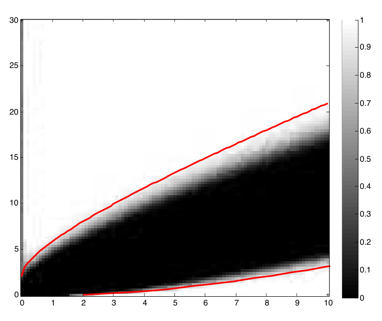
Now we present our simulation results for exact recovery and misclassification rates of SBM. The phase transition phenomenon of SBM is exhibited on the left of Figure 6. In this simulation, nn is fixed as 300300, and parameters aa (yy-axis) and bb (xx-axis) vary from 00 to 3030 and 00 to 1010, with increments 0.30.3 and 0.10.1 respectively. We compare the labels returned by our eigenvector-based method with the true cluster labels, and report the the proportion of success (namely z^=±z\hat{z}=\pm z) out of 100100 independent runs. As before, lighter pixels represent higher chances of success. Two theoretical curves a−b=±2\sqrt{a}-\sqrt{b}=\pm\sqrt{2} are also added onto the heat map. Clearly, theoretical predictions match numerical results.

The right plot of Figure 6 shows misclassification rates of our eigenvector approach with a fixed parameter bb and a varying parameter aa, where aa is not large enough to reach the exact recovery threshold. We fix b=2b=2, and increase aa from 22 to 88 by 0.20.2 for three different choices of nn from {100,500,5000}\{100,500,5000\}. Then we calculate the mean misclassification rates 𝔼​r​(z^,z)\mathbb{E}r(\hat{z},z) averaged over 100100 independent runs, and plot log⁡𝔼​r​(z^,z)/log⁡n\log\mathbb{E}r(\hat{z},z)/\log n against varying bb. We also add a theoretical curve (with no markers), whose yy-coordinates are −(a−b)2/2-(\sqrt{a}-\sqrt{b})^{2}/2; see Theorem 3.2 (ii). It is clear that with nn tending to infinity, the curves of mean misclassification rates move closer to the theoretical one.
Refer to caption
Figure 6: Vanilla spectral method for SBM. Left: phase transition of exact recovery. The xx-axis is bb, the yy-axis is aa, and lighter pixels represent higher chances of success. Two red curves a−b=±2\sqrt{a}-\sqrt{b}=\pm\sqrt{2} represent theoretical boundaries for phase transtion, matched by numerical results. Right: mean misclassification rates on the logarithmic scale with b=2b=2. The xx-axis is aa, varying from 22 to 88, and the yy-axis is log⁡𝔼​r​(z^,z)/log⁡n\log\mathbb{E}r(\hat{z},z)/\log n. No marker: theoretical curve; circles: n=5000n=5000; crosses: n=500n=500; squares: n=100n=100.

4.3 Matrix completion from noisy entries

Finally we come to experiments of matrix completion from noisy entries. The performance of the spectral algorithm in terms of root-mean squared error (RMSE) has already been demonstrated in Keshavan et al. (2010b), among others. In this part, we focus on the comparison between the maximum entrywise errors and RMSEs, for both the singular vectors and the matrix itself. The settings are mainly adopted from Candès and Plan (2010) and Keshavan et al. (2010b). Each time we first create a rank-rr matrix M∗∈ℝn×nM^{*}\in\mathbb{R}^{n\times n} using the product ML​MRTM_{L}M_{R}^{T}, where ML,MR∈ℝn×rM_{L},M_{R}\in\mathbb{R}^{n\times r} have i.i.d. N⁡(0,20/n)N(0,20/\sqrt{n}) entries. Then, each entry of M∗M^{*} is picked with probability pp and contaminated by random noise drawn from N⁡(0,σ2)N(0,\sigma^{2}), independently of others. While increasing nn from 500500 to 50005000 by 500500, we choose p=10​log⁡nnp=\frac{10\log n}{n}, fix r=5r=5 and σ=1\sigma=1. All the data presented in the plot are averaged over 100100 independent experiments.

In support of our discussions in Section 3.3, Figure 7 shows that the following two ratios

Rmat=‖U​Σ​VT−M∗‖maxη2​log⁡n⋅‖U​Σ​VT−M∗‖F,\displaystyle R_{\mathrm{mat}}=\frac{\|U\Sigma V^{T}-M^{*}\|_{\max}}{\eta^{2}\sqrt{\log n}\cdot\|U\Sigma V^{T}-M^{*}\|_{F}},
Rvec=max⁡{‖U​sgn​(H)−U∗‖2→∞,‖V​sgn​(H)−V∗‖2→∞}η​log⁡n⋅max⁡{‖U​sgn​(H)−U∗‖F,‖V​sgn​(H)−V∗‖F},\displaystyle R_{\mathrm{vec}}=\frac{\max\{\|U\mathrm{sgn}(H)-U^{*}\|_{2\to\infty},\|V\mathrm{sgn}(H)-V^{*}\|_{2\to\infty}\}}{\eta\sqrt{\log n}\cdot\max\{\|U\mathrm{sgn}(H)-U^{*}\|_{F},\|V\mathrm{sgn}(H)-V^{*}\|_{F}\}},

approximately remain constant as nn grows. Here the RMSEs n−1​‖U​Σ​VT−M∗‖Fn^{-1}\|U\Sigma V^{T}-M^{*}\|_{F} and n−1/2max{∥Usgn(H)−U∗∥F,∥Vsgn(H)−V∗∥F}n^{-1/2}\max\{\|U\mathrm{sgn}(H)-U^{*}\|_{F},\|V\mathrm{sgn}(H)-V^{*}\|_{F}\} are scaled by (n​η)2​log⁡n(\sqrt{n}\eta)^{2}\sqrt{\log n} and (n​η)​log⁡n(\sqrt{n}\eta)\sqrt{\log n}, respectively. Hence our analysis is sharp, and the perturbations are obviously delocalized among the entries.

Figure 7: RmatR_{\mathrm{mat}} and RvecR_{\mathrm{vec}} in matrix completion from noisy entries. The xx-axis is nn, varying from 500500 to 50005000 by 500500, and the yy-axis is the ratio. Crosses and circles stand for RmatR_{\mathrm{mat}} and RvecR_{\mathrm{vec}}, respectively.

5 Discussions

We have developed first-order approximations for eigenvectors and eigenspaces with small ℓ∞\ell_{\infty} errors under random perturbations. These results lead to sharp guarantees for three statistical problems.

Several future directions deserve exploration. First, the main perturbation theorems are currently stated only for symmetric matrices. We think it may be possible to extend the current analysis to SVD of general rectangular matrices, which has broader applications such as principal component analysis. Second, there are many other graph-related matrices beyond adjacency matrices, including graph Laplacians and non-backtracking matrices, which are important both in theory and in practice. Third, we believe our assumption of row- and column-wise independence can be relaxed to block-wise independence, which is relevant to cryo-EM and other problems.

Finally, in our examples, the spectral algorithm is strongly consistent if and only if the MLE is, though the latter can be NP-hard to compute in general. It would be interesting to see how general this phenomenon is, in view of better understanding the statistical and computational tradeoffs.

Acknowledgements

The authors thank Harrison Zhou, Amit Singer, Nicolas Boumal, Yuxin Chen and Cong Ma for helpful discussions.

Appendix A Outline of proofs

In this section, we first present key observations leading to the inequalities (2.6) and (2.7) for the eigenvector case. The analysis and insights for eigenvector perturbation will be instrumental for the general eigenspace perturbation result. Then, we outline the proof ideas for Theorem 2.1.

A.1 Warm-up analysis of eigenvector perturbation

Let us consider the simpler setting in Section 2.2: we assume a rank-one structure: A∗=λ∗​u∗​(u∗)TA^{*}=\lambda^{*}u^{*}(u^{*})^{T} (dropping the subscript for simplicity). By Weyl’s inequality, the leading eigenvalue λ\lambda of AA satisfies |λ−λ∗|≤‖A−A∗‖2|\lambda-\lambda^{*}|\leq\|A-A^{*}\|_{2}, and by the spectral norm concentration Assumption A3, we obtain |λ−λ∗|≤‖A−A∗‖2≤γ​λ∗|\lambda-\lambda^{*}|\leq\|A-A^{*}\|_{2}\leq\gamma\lambda^{*}. Note γ<1/2\gamma<1/2 under Assumption A3, so λ≥λ∗/2\lambda\geq\lambda^{*}/2. By the triangle inequality, we have

‖u‖∞=‖A​uλ‖∞≤‖A​u∗λ‖∞+‖A⁡(u−u∗)λ‖∞≤2λ∗​(‖A​u∗‖∞+‖A⁡(u−u∗)‖∞).\displaystyle\|u\|_{\infty}=\left\|\frac{Au}{\lambda}\right\|_{\infty}\leq\left\|\frac{Au^{*}}{\lambda}\right\|_{\infty}+\left\|\frac{A(u-u^{*})}{\lambda}\right\|_{\infty}\leq\frac{2}{\lambda^{*}}\left(\|Au^{*}\|_{\infty}+\|A(u-u^{*})\|_{\infty}\right). (A.1)

Likewise, using u=A​u/λu=Au/\lambda and |λ−1−(λ∗)−1|=|λ−λ∗|/|λ​λ∗|≤2​γ/λ∗|\lambda^{-1}-(\lambda^{*})^{-1}|=|\lambda-\lambda^{*}|/|\lambda\lambda^{*}|\leq 2\gamma/\lambda^{*}, we have

‖u−A​u∗λ∗‖∞≤|1λ−1λ∗|​‖A​u∗‖∞+1λ​‖A⁡(u−u∗)‖∞≤2λ∗​(γ​‖A​u∗‖∞+‖A⁡(u−u∗)‖∞)\displaystyle\left\|u-\frac{Au^{*}}{\lambda^{*}}\right\|_{\infty}\leq\left|\frac{1}{\lambda}-\frac{1}{\lambda^{*}}\right|\left\|Au^{*}\right\|_{\infty}+\frac{1}{\lambda}\left\|A(u-u^{*})\right\|_{\infty}\leq\frac{2}{\lambda^{*}}\left(\gamma\|Au^{*}\|_{\infty}+\|A(u-u^{*})\|_{\infty}\right) (A.2)

Note that A​u∗=λ∗​u∗+(A−A∗)​u∗Au^{*}=\lambda^{*}u^{*}+(A-A^{*})u^{*}, so it is easy to bound ‖A​u∗‖∞\|Au^{*}\|_{\infty} using the row concentration assumption: in Assumption A4, we set w=u∗w=u^{*}, and the row concentration inequality (2.3) and the union bound imply ‖(A−A∗)​u∗‖∞≤λ∗​φ​(1)​‖u∗‖∞\|(A-A^{*})u^{*}\|_{\infty}\leq\lambda^{*}\varphi(1)\|u^{*}\|_{\infty} with probability 1−δ1/r1-\delta_{1}/r (recall Δ∗=λ∗\Delta^{*}=\lambda^{*}). Then, the goal is to obtain a good bound on ‖A⁡(u−u∗)‖∞\|A(u-u^{*})\|_{\infty}.

However, the random quantities AA and u−u∗u-u^{*} are dependent, and we cannot directly use the row concentration assumption. To resolve this issue, we use a leave-one-out technique similar to the ones in Bean et al. (2013), Javanmard and Montanari (2015), and Zhong and Boumal (2018). Define nn auxiliary matrices A(1),A(2),⋯,A(n)∈ℝn×nA^{(1)},A^{(2)},\cdots,A^{(n)}\in\mathbb{R}^{n\times n} as follows: for any m∈[n]m\in[n], let

[A(m)]i​j=Ai​j​𝟏{i≠m,j≠m},[A^{(m)}]_{ij}=A_{ij}\mathbf{1}_{\{i\neq m,j\neq m\}}, (A.3)

where 𝟏\mathbf{1} is the indicator function. By definition, for all m∈[n]m\in[n], A(m)A^{(m)} is a symmetric matrix, and its entries are identical to those of AA except that entries in its mmth row and column are zero. The row and column-wise independence Assumption A2 then implies that A−A(m)A-A^{(m)} and A(m)A^{(m)} are independent. This simple observation is the cornerstone to decouple dependence.

For each m∈[n]m\in[n], let u(m)u^{(m)} be the leading eigenvector of A(m)A^{(m)} with the appropriately chosen sign. By the triangle inequality and the definition of ∥⋅∥2→∞\|\cdot\|_{2\to\infty}, we have

|[A⁡(u−u∗)]m|\displaystyle|[A(u-u^{*})]_{m}| =|Am⋅(u−u∗)|≤|Am⋅(u−u(m))|+|Am⋅(u(m)−u∗)|\displaystyle=|A_{m\cdot}(u-u^{*})|\leq|A_{m\cdot}(u-u^{(m)})|+|A_{m\cdot}(u^{(m)}-u^{*})| (A.4)
≤∥A∥2→∞∥u−u(m)∥2+|Am⋅(u(m)−u∗)|.\displaystyle\leq\|A\|_{2\to\infty}\|u-u^{(m)}\|_{2}+|A_{m\cdot}(u^{(m)}-u^{*})|. (A.5)

Here recall Am⋅A_{m\cdot} is the mmth row vector of AA. The advantage of introducing u(m)u^{(m)} is pronounced in the second term of (A.5): the mmth row Am⋅A_{m\cdot} and u(m)−u∗u^{(m)}-u^{*} are independence. This is because by definition, u(m)u^{(m)} only depends on A(m)A^{(m)} and thus is independent of Am⋅A_{m\cdot}. Using the row concentration Assumption A4, we can show that |Am⋅(u(m)−u∗)|≲λ∗(γ+φ(γ))(∥u∥∞+∥u∗∥∞)|A_{m\cdot}(u^{(m)}-u^{*})|\lesssim\lambda^{*}(\gamma+\varphi(\gamma))(\|u\|_{\infty}+\|u^{*}\|_{\infty}). The term ‖u‖∞\|u\|_{\infty} will ultimately be absorbed into the left-hand side of (A.1) after rearrangement.

A crucial step in the proof is a sharp bound on ‖u−u(m)‖2\|u-u^{(m)}\|_{2}. Viewing u(m)u^{(m)} as a perturbed version of uu, we use a (proper) form of Davis-Kahan’s sin⁡Θ\sin\Theta theorem (Davis and Kahan, 1970) to obtain

‖u−u(m)‖2≲‖(A−A(m))​u‖2λ∗=‖v‖2λ∗,where ​v:=(A−A(m))​u.\|u-u^{(m)}\|_{2}\lesssim\frac{\|(A-A^{(m)})u\|_{2}}{\lambda^{*}}=\frac{\|v\|_{2}}{\lambda^{*}},\qquad\text{where }v:=(A-A^{(m)})u.

An important feature of this bound is that, in the numerator, A−A(m)A-A^{(m)} only has nonzero entries in the mmth row and mmth column. Consider bounding mmth entry of vv and its other entries separately, we have

|vm|=|Am⋅u|=|[Au]m|=|λum|≤|λ|∥u∥∞,\displaystyle|v_{m}|=|A_{m\cdot}u|=|[Au]_{m}|=|\lambda u_{m}|\leq|\lambda|\|u\|_{\infty},
(∑i≠mvi2)1/2=(∑i≠mAm​i2​um2)1/2≤‖A‖2→∞​‖u‖∞≤2​γ​|λ∗|​‖u‖∞,\displaystyle\Big(\sum_{i\neq m}v_{i}^{2}\Big)^{1/2}=\Big(\sum_{i\neq m}A_{mi}^{2}u_{m}^{2}\Big)^{1/2}\leq\|A\|_{2\to\infty}\|u\|_{\infty}\leq 2\gamma|\lambda^{*}|\|u\|_{\infty},

where the last inequality is due to ‖A‖2→∞≤‖A∗‖2→∞+‖A−A∗‖2≤2​γ​λ∗\|A\|_{2\to\infty}\leq\|A^{*}\|_{2\to\infty}+\|A-A^{*}\|_{2}\leq 2\gamma\lambda^{*} under Assumption A1 and A3. This will lead to a sharp bound ‖u−u(m)‖2≲‖u‖∞\|u-u^{(m)}\|_{2}\lesssim\|u\|_{\infty}, and therefore a good control of the first term of (A.5):

‖A‖2→∞​‖u−u(m)‖2≲γ​λ∗​‖u‖∞.\|A\|_{2\to\infty}\|u-u^{(m)}\|_{2}\lesssim\gamma\lambda^{*}\|u\|_{\infty}. (A.6)

After rearrangement of (A.1), the terms involving ‖u‖∞\|u\|_{\infty} will be absorbed into the left-hand side, and we will obtain the first inequality (2.6). Once (2.6) is proved, we can then bound the two terms in (A.5) in terms of ‖u∗‖∞\|u^{*}\|_{\infty}:

‖A‖2→∞​‖u−u(m)‖2≲γ​λ∗​(1+φ⁡(1))​‖u∗‖∞,\displaystyle\|A\|_{2\to\infty}\|u-u^{(m)}\|_{2}\lesssim\gamma\lambda^{*}(1+\varphi(1))\|u^{*}\|_{\infty},
|Am⋅(u(m)−u∗)|≲λ∗(γ+φ(γ))(1+φ(1))∥u∗∥∞.\displaystyle|A_{m\cdot}(u^{(m)}-u^{*})|\lesssim\lambda^{*}(\gamma+\varphi(\gamma))(1+\varphi(1))\|u^{*}\|_{\infty}.

Using the above two bounds, together with the bound on ‖A​u∗‖∞\|Au^{*}\|_{\infty}, we simplify (A.2) and derive

‖u−A​u∗λ∗‖∞≲γ​φ​(1)​‖u∗‖∞+(γ+φ⁡(γ))​(1+φ⁡(1))​‖u∗‖∞,\left\|u-\frac{Au^{*}}{\lambda^{*}}\right\|_{\infty}\lesssim\gamma\varphi(1)\|u^{*}\|_{\infty}+(\gamma+\varphi(\gamma))(1+\varphi(1))\|u^{*}\|_{\infty},

which leads to the second inequality (2.7).

A.2 Proof ideas for Theorem 2.1

Unlike the eigenvector case, the eigenspaces are up to a orthogonal matrix, so we have to study HH and sgn⁡(H)\mathrm{sgn}(H). Some basic properties about HH are stated in Lemma 2. Moreover, following the decoupling idea in A.1, for each m∈[n]m\in[n], we let U(m)=[us+1(m),⋯,us+r(m)]∈ℝn×rU^{(m)}=[u^{(m)}_{s+1},\cdots,u^{(m)}_{s+r}]\in\mathbb{R}^{n\times r} be the similar matrix as UU. And in addition, we define additional nn auxiliary matrices H(1),H(2),⋯,H(n)∈ℝr×rH^{(1)},H^{(2)},\cdots,H^{(n)}\in\mathbb{R}^{r\times r}:

H(m)=[U(m)]T​U∗.H^{(m)}=[U^{(m)}]^{T}U^{*}. (A.7)

The purpose of introducing U(m)U^{(m)} and H(m)H^{(m)} is to ensure independence—see the comments below (A.5). The next lemma is a deterministic result, in parallel with the inequalities (A.1) and (A.2) derived for the eigenvector case.

Lemma 1.

Let γ¯=‖E‖2/Δ∗\bar{\gamma}=\|E\|_{2}/\Delta^{*}. If γ¯≤1/10\bar{\gamma}\leq 1/10, then for any m∈[n]m\in[n] we have

∥(UH)m⋅∥2≤2Δ∗(∥Am⋅U∗∥2+∥Am⋅(UH−U∗)∥2),\displaystyle\|(UH)_{m\cdot}\|_{2}\leq\frac{2}{\Delta^{*}}(\|A_{m\cdot}U^{*}\|_{2}+\|A_{m\cdot}(UH-U^{*})\|_{2}), (A.8)
‖(UH−AU∗(Λ∗)−1)m⋅‖2≤6​γ¯Δ∗∥Am⋅U∗∥2+2Δ∗∥Am⋅(UH−U∗)∥2.\displaystyle\left\|{(UH-AU^{*}(\Lambda^{*})^{-1})_{m\cdot}}\right\|_{2}\leq\frac{6\bar{\gamma}}{\Delta^{*}}\|A_{m\cdot}U^{*}\|_{2}+\frac{2}{\Delta^{*}}\|A_{m\cdot}(UH-U^{*})\|_{2}. (A.9)

The proof of Lemma 1, which is in the appendix, is technical by nature. This is caused by the fact that HH and Λ\Lambda are not commutative (whereas in the eigenvector case, H=uT​u∗∈ℝH=u^{T}u^{*}\in\mathbb{R} and λ\lambda is commutative). By Lemma 1 and the triangle inequality, we have the following bound for all mm’s, which is similar to (A.4):

∥(UH)m⋅∥2≤2Δ∗(∥Am⋅U∗∥2+∥Am⋅(UH−U∗)∥2)\displaystyle\|(UH)_{m\cdot}\|_{2}\leq\frac{2}{\Delta^{*}}(\|A_{m\cdot}U^{*}\|_{2}+\|A_{m\cdot}(UH-U^{*})\|_{2})
≤2Δ∗(∥Am⋅U∗∥2+∥Am⋅(UH−U(m)H(m))∥2+∥Am⋅(U(m)H(m)−U∗)∥2).\displaystyle\leq\frac{2}{\Delta^{*}}\left(\|A_{m\cdot}U^{*}\|_{2}+\|A_{m\cdot}(UH-U^{(m)}H^{(m)})\|_{2}+\|A_{m\cdot}(U^{(m)}H^{(m)}-U^{*})\|_{2}\right). (A.10)

A deterministic argument shows that the second term in (A.10), namely 2(Δ∗)−1∥Am⋅(UH−U(m)H(m))∥22(\Delta^{*})^{-1}\|A_{m\cdot}(UH-U^{(m)}H^{(m)})\|_{2}, is a vanishing proportion of ∥(UH)m⋅∥2\|(UH)_{m\cdot}\|_{2}, so after rearrangement, we only need to bound the first term and the third term—see (B.10) and (B.11) in Lemma 3. This is similar to the derivation of (A.6), in which we use a proper form of Davis-Kahan’s theorem. The first term, by the row concentration Assumption A4, can be controlled fairly easily—see Lemma 4. The third term, by the row concentration assumption again, can be bounded by a vanishing proportion of ‖U​H‖2→∞+‖U∗‖2→∞\|UH\|_{2\to\infty}+\|U^{*}\|_{2\to\infty}, and finally, this leads to a bound on ‖U​H‖2→∞\|UH\|_{2\to\infty} after rearranging (A.10). It is vital that the function φ⁡(x)\varphi(x) in the row concentration assumption sharply captures the concentration for non-uniform weights, and this allows a good control of the third term—see Lemma 5.

All these arguments lead to a bound on ‖U​H‖2→∞\|UH\|_{2\to\infty} that is roughly O⁡(‖U∗‖2→∞+‖A∗‖2→∞/Δ∗)O(\|U^{*}\|_{2\to\infty}+\|A^{*}\|_{2\to\infty}/\Delta^{*}), and in many applications, this is O⁡(‖U∗‖2→∞)O(\|U^{*}\|_{2\to\infty}). In other words, this says ‖U​H‖2→∞\|UH\|_{2\to\infty} inflates ‖U∗‖2→∞\|U^{*}\|_{2\to\infty} by at most a constant factor.

Similar to the eigenvector case, the bound on ‖U​H‖2→∞\|UH\|_{2\to\infty} finally leads to a sharp bound on ‖U​H−A​U∗​(Λ∗)−1‖2→∞\|UH-AU^{*}(\Lambda^{*})^{-1}\|_{2\to\infty}, and thus proves Theorem 2.1. To understand this, assuming ‖A−A∗‖2≤γ​Δ∗\|A-A^{*}\|_{2}\leq\gamma\Delta^{*}, which happens with probability at least 1−δ01-\delta_{0}, the triangle inequality yields

‖U​H−A​U∗​(Λ∗)−1‖2→∞\displaystyle\|UH-AU^{*}(\Lambda^{*})^{-1}\|_{2\to\infty} ≤6​γΔ∗∥AU∗∥2→∞+2Δ∗maxm∈[n]∥Am⋅(UH−U(m)H(m))∥2\displaystyle\leq\frac{6\gamma}{\Delta^{*}}\|AU^{*}\|_{2\to\infty}+\frac{2}{\Delta^{*}}\max\limits_{m\in[n]}\|A_{m\cdot}(UH-U^{(m)}H^{(m)})\|_{2}
+2Δ∗maxm∈[n]∥Am⋅(U(m)H(m)−U∗)∥2.\displaystyle+\frac{2}{\Delta^{*}}\max\limits_{m\in[n]}\|A_{m\cdot}(U^{(m)}H^{(m)}-U^{*})\|_{2}. (A.11)

As argued above, we can bound the first term and the second term using Lemma 3 and 4. Now that we have a bound on ‖U​H‖2→∞\|UH\|_{2\to\infty}, Lemma 5 immediately implies that with probability 1−δ11-\delta_{1}, the third term is a small proportion of that bound, or equivalently O⁡((γ+φ⁡(γ))​(‖U∗‖max+‖A∗‖2→∞/Δ∗))O((\gamma+\varphi(\gamma))(\|U^{*}\|_{\max}+\|A^{*}\|_{2\to\infty}/\Delta^{*})). Note that, if γ=o⁡(1)\gamma=o(1) as n→∞n\to\infty, the final bound is an order smaller than ‖U∗‖max+‖A∗‖2→∞/Δ∗\|U^{*}\|_{\max}+\|A^{*}\|_{2\to\infty}/\Delta^{*}.

Appendix B Proofs for Section 2

B.1 Deterministic lemmas

This subsection states and proves deterministic results useful for the proof. We temporarily ignore Assumptions A2-A4 and may only assume A1. First we present basic properties of H=UT​U∗H=U^{T}U^{*}, which is shown to be close to the orthonormal matrix sgn⁡(H)\mathrm{sgn}(H). Both of them play an important role in aligning UU with U∗U^{*}. The techniques used in dealing with HH and sgn⁡(H)\mathrm{sgn}(H) are similar to the ones in Fan et al. (2017).

Lemma 2.

‖H‖2≤1\|H\|_{2}\leq 1. When γ¯=‖E‖2/Δ∗≤1\bar{\gamma}=\|E\|_{2}/\Delta^{*}\leq 1, we have

‖H−sgn⁡(H)‖21/2≤‖U​UT−U∗​(U∗)T‖2≤‖E​U∗‖2(1−γ¯)​Δ∗≤γ¯1−γ¯,\|H-\mathrm{sgn}(H)\|_{2}^{1/2}\leq\|UU^{T}-U^{*}(U^{*})^{T}\|_{2}\leq\frac{\|EU^{*}\|_{2}}{(1-\bar{\gamma})\Delta^{*}}\leq\frac{\bar{\gamma}}{1-\bar{\gamma}}, (B.1)

and ‖Λ​H−H​Λ‖2≤2​‖E‖2\|\Lambda H-H\Lambda\|_{2}\leq 2\|E\|_{2}. When γ¯≤1/2\bar{\gamma}\leq 1/2, we have ‖H−1‖2≤(1−γ¯)2/(1−2​γ¯)\left\|{H^{-1}}\right\|_{2}\leq(1-\bar{\gamma})^{2}/(1-2\bar{\gamma}) and

‖Um⋅(HΛ−ΛH)‖2≤2​(1−γ¯)21−2​γ¯∥E∥2‖(UH)m⋅‖2,∀m∈[n].\left\|{U_{m\cdot}(H\Lambda-\Lambda H)}\right\|_{2}\leq\frac{2(1-\bar{\gamma})^{2}}{1-2\bar{\gamma}}\|E\|_{2}\left\|{(UH)_{m\cdot}}\right\|_{2},~\forall m\in[n]. (B.2)
Proof of Lemma 2.

First, we have ‖H‖2=‖UT​U∗‖2≤‖UT‖2​‖U∗‖2=1\|H\|_{2}=\|U^{T}U^{*}\|_{2}\leq\|U^{T}\|_{2}\|U^{*}\|_{2}=1. Let the SVD of H=UT​U∗H=U^{T}U^{*} be U¯​Σ¯​V¯T\bar{U}\bar{\Sigma}\bar{V}^{T}, where U¯,V¯∈ℝr×r\bar{U},\bar{V}\in\mathbb{R}^{r\times r} are orthogonal matrices and Σ¯=diag⁡{σ¯1,⋯,σ¯r}\bar{\Sigma}=\mathrm{diag}\{\bar{\sigma}_{1},\cdots,\bar{\sigma}_{r}\} is a diagonal matrix. Then sgn⁡(H)=U¯​V¯T\mathrm{sgn}(H)=\bar{U}\bar{V}^{T}. By (Stewart and Sun, 1990, Chp I, Cor 5.4), the singular values 1≥σ¯1≥⋯≥σ¯r≥01\geq\bar{\sigma}_{1}\geq\cdots\geq\bar{\sigma}_{r}\geq 0 are the cosines of canonical angles 0≤θ¯1≤⋯≤θ¯r≤π/20\leq\bar{\theta}_{1}\leq\cdots\leq\bar{\theta}_{r}\leq\pi/2 between the column spaces of UU and U∗U^{*}. We have ‖sgn⁡(H)−H‖2=1−cos⁡θ¯r\|\mathrm{sgn}(H)-H\|_{2}=1-\cos\bar{\theta}_{r}.

The Davis-Kahan sin⁡Θ\sin\Theta theorem (Davis and Kahan, 1970) forces sin⁡θ¯r≤‖U∗​(U∗)T​E‖2/δ≤‖E​U∗‖2/δ\sin\bar{\theta}_{r}\leq\left\|{U^{*}(U^{*})^{T}E}\right\|_{2}/\delta\leq\left\|{EU^{*}}\right\|_{2}/\delta, where δ=(λs−λs+1∗)+∧(λs+r∗−λs+r+1)+\delta=(\lambda_{s}-\lambda_{s+1}^{*})_{+}\wedge(\lambda_{s+r}^{*}-\lambda_{s+r+1})_{+} and we define x+=x∨0x_{+}=x\vee 0 for x∈ℝx\in\mathbb{R}. On the one hand, Weyl’s inequality (Stewart and Sun, 1990, Chp IV, Cor 4.9) leads to δ≥Δ∗−‖E‖2≥(1−γ¯)​Δ∗\delta\geq\Delta^{*}-\|E\|_{2}\geq(1-\bar{\gamma})\Delta^{*}. On the other hand, sin⁡θ¯r=‖U​UT−U∗​(U∗)T‖2\sin\bar{\theta}_{r}=\|UU^{T}-U^{*}(U^{*})^{T}\|_{2} follows from (Stewart and Sun, 1990, Chp I, Thm 5.5). Besides, θ¯r∈[0,π/2]\bar{\theta}_{r}\in[0,\pi/2] forces 0≤cos⁡θ¯r≤10\leq\cos\bar{\theta}_{r}\leq 1, cos⁡θ¯r≥cos2⁡θ¯r=1−sin2⁡θ¯r\cos\bar{\theta}_{r}\geq\cos^{2}\bar{\theta}_{r}=1-\sin^{2}\bar{\theta}_{r} and

‖H−sgn⁡(H)‖21/2=1−cos⁡θ¯r≤sin⁡θ¯r=‖U​UT−U∗​(U∗)T‖2≤‖E​U∗‖2(1−γ¯)​Δ∗≤γ¯1−γ¯.\|H-\mathrm{sgn}(H)\|_{2}^{1/2}=\sqrt{1-\cos\bar{\theta}_{r}}\leq\sin\bar{\theta}_{r}=\|UU^{T}-U^{*}(U^{*})^{T}\|_{2}\leq\frac{\|EU^{*}\|_{2}}{(1-\bar{\gamma})\Delta^{*}}\leq\frac{\bar{\gamma}}{1-\bar{\gamma}}.

Note that UT​A=Λ​UTU^{T}A=\Lambda U^{T} and A∗​U∗=U∗​Λ∗A^{*}U^{*}=U^{*}\Lambda^{*}. We have

UT​E​U∗=UT​A​U∗−UT​A∗​U∗=Λ​UT​U∗−UT​U∗​Λ∗=Λ​H−H​Λ∗.U^{T}EU^{*}=U^{T}AU^{*}-U^{T}A^{*}U^{*}=\Lambda U^{T}U^{*}-U^{T}U^{*}\Lambda^{*}=\Lambda H-H\Lambda^{*}.

By the triangle inequality,

‖Λ​H−H​Λ‖2=‖UT​E​U∗+H⁡(Λ∗−Λ)‖2≤‖UT​E​U∗‖2+‖H⁡(Λ∗−Λ)‖2≤2​‖E‖2,\|\Lambda H-H\Lambda\|_{2}=\|U^{T}EU^{*}+H(\Lambda^{*}-\Lambda)\|_{2}\leq\|U^{T}EU^{*}\|_{2}+\|H(\Lambda^{*}-\Lambda)\|_{2}\leq 2\|E\|_{2},

where we used ‖Λ−Λ∗‖2≤‖E‖2\|\Lambda-\Lambda^{*}\|_{2}\leq\left\|{E}\right\|_{2} and ‖H‖2≤1\|H\|_{2}\leq 1.

From now on we assume that γ¯≤1/2\bar{\gamma}\leq 1/2. ‖H−sgn⁡(H)‖2≤[γ¯/(1−γ¯)]2≤1\|H-\mathrm{sgn}(H)\|_{2}\leq[\bar{\gamma}/(1-\bar{\gamma})]^{2}\leq 1 leads to

‖H−1−sgn​(H)−1‖2≤‖sgn​(H)−1​[H−sgn⁡(H)]‖21−‖sgn​(H)−1​[H−sgn⁡(H)]‖2≤‖H−sgn⁡(H)‖21−‖H−sgn⁡(H)‖2≤γ¯21−2​γ¯,\displaystyle\|H^{-1}-\mathrm{sgn}(H)^{-1}\|_{2}\leq\frac{\|\mathrm{sgn}(H)^{-1}[H-\mathrm{sgn}(H)]\|_{2}}{1-\|\mathrm{sgn}(H)^{-1}[H-\mathrm{sgn}(H)]\|_{2}}\leq\frac{\|H-\mathrm{sgn}(H)\|_{2}}{1-\|H-\mathrm{sgn}(H)\|_{2}}\leq\frac{\bar{\gamma}^{2}}{1-2\bar{\gamma}},
‖H−1‖2≤‖sgn​(H)−1‖2+‖H−1−sgn​(H)−1‖2≤1+γ¯21−2​γ¯=(1−γ¯)21−2​γ¯.\displaystyle\|H^{-1}\|_{2}\leq\|\mathrm{sgn}(H)^{-1}\|_{2}+\|H^{-1}-\mathrm{sgn}(H)^{-1}\|_{2}\leq 1+\frac{\bar{\gamma}^{2}}{1-2\bar{\gamma}}=\frac{(1-\bar{\gamma})^{2}}{1-2\bar{\gamma}}.

Finally we come to the last claim.

‖Um⋅(HΛ−ΛH)‖2\displaystyle\left\|{U_{m\cdot}(H\Lambda-\Lambda H)}\right\|_{2} =‖(UH)m⋅H−1(HΛ−ΛH)‖2≤‖(UH)m⋅‖2‖H−1‖2‖HΛ−ΛH‖2\displaystyle=\left\|{(UH)_{m\cdot}H^{-1}(H\Lambda-\Lambda H)}\right\|_{2}\leq\left\|{(UH)_{m\cdot}}\right\|_{2}\left\|{H^{-1}}\right\|_{2}\left\|{H\Lambda-\Lambda H}\right\|_{2}
≤‖(UH)m⋅‖2⋅(1−γ¯)21−2​γ¯⋅2‖E‖2.\displaystyle\leq\left\|{(UH)_{m\cdot}}\right\|_{2}\cdot\frac{(1-\bar{\gamma})^{2}}{1-2\bar{\gamma}}\cdot 2\left\|{E}\right\|_{2}.

∎

Next, we prove Lemma 1. This will soon leads to simplified bounds in Lemma 3.

Proof of Lemma 1.

Define Λ=diag⁡(λs+1,⋯,λs+r)∈ℝr×r\Lambda=\mathrm{diag}(\lambda_{s+1},\cdots,\lambda_{s+r})\in\mathbb{R}^{r\times r}. By Weyl’s inequality, maxi∈[r]⁡|λs+i−λs+i∗|=‖Λ−Λ∗‖2≤‖E‖2≤γ¯​Δ∗\max_{i\in[r]}|\lambda_{s+i}-\lambda_{s+i}^{*}|=\|\Lambda-\Lambda^{*}\|_{2}\leq\left\|{E}\right\|_{2}\leq\bar{\gamma}\Delta^{*}, and so mini∈[r]⁡|λs+i|≥(1−γ¯)​Δ∗\min_{i\in[r]}|\lambda_{s+i}|\geq(1-\bar{\gamma})\Delta^{*}. Moreover, since A​U=U​ΛAU=U\Lambda, we have

U​H​Λ−A​U∗=U⁡(H​Λ−Λ​H)+A⁡(U​H−U∗).UH\Lambda-AU^{*}=U(H\Lambda-\Lambda H)+A(UH-U^{*}). (B.3)

Note that when r=1r=1, HH and Λ\Lambda are scalars, so the term involving H​Λ−Λ​HH\Lambda-\Lambda H vanishes. By the triangle inequality and Weyl’s inequality, the entries of UU are easy to bound. However, for a general rr, the trouble that HH and Λ\Lambda do not commute requires more work.

We multiply (B.3) by Λ−1\Lambda^{-1} on the right, use Lemma 2 and the triangle inequality to derive

∥(UH−AU∗Λ−1)m⋅∥2\displaystyle\|(UH-AU^{*}\Lambda^{-1})_{m\cdot}\|_{2} ≤∥Um⋅(HΛ−ΛH)Λ−1∥2+∥Am⋅(UH−U∗)Λ−1∥2\displaystyle\leq\|U_{m\cdot}(H\Lambda-\Lambda H)\Lambda^{-1}\|_{2}+\|A_{m\cdot}(UH-U^{*})\Lambda^{-1}\|_{2}
≤1mini∈[r]⁡|λs+i|(2​(1−γ¯)21−2​γ¯∥E∥2∥(UH)m⋅∥2+∥Am⋅(UH−U∗)∥2)\displaystyle\leq\frac{1}{\min_{i\in[r]}|\lambda_{s+i}|}\left(\frac{2(1-\bar{\gamma})^{2}}{1-2\bar{\gamma}}\|E\|_{2}\|(UH)_{m\cdot}\|_{2}+\|A_{m\cdot}(UH-U^{*})\|_{2}\right)
≤2​γ¯1−2​γ¯∥(UH)m⋅∥2+1(1−γ¯)​Δ∗∥Am⋅(UH−U∗)∥2.\displaystyle\leq\frac{2\bar{\gamma}}{1-2\bar{\gamma}}\|(UH)_{m\cdot}\|_{2}+\frac{1}{(1-\bar{\gamma})\Delta^{*}}\|A_{m\cdot}(UH-U^{*})\|_{2}. (B.4)

On the other hand,

∥(UH−AU∗Λ−1)m⋅∥2≥‖(UH)m⋅‖2−∥Am⋅U∗∥2mini∈[r]⁡|λs+i|≥‖(UH)m⋅‖2−‖Am⋅U∗‖2(1−γ¯)​Δ∗.\|(UH-AU^{*}\Lambda^{-1})_{m\cdot}\|_{2}\geq\left\|{(UH)_{m\cdot}}\right\|_{2}-\frac{\|A_{m\cdot}U^{*}\|_{2}}{\min_{i\in[r]}|\lambda_{s+i}|}\geq\left\|{(UH)_{m\cdot}}\right\|_{2}-\frac{\left\|{A_{m\cdot}U^{*}}\right\|_{2}}{(1-\bar{\gamma})\Delta^{*}}. (B.5)

Combining this bound with (B.4),

∥(UH)m⋅∥2≤1−2​γ¯(1−γ¯)​(1−4​γ¯)⋅1Δ∗(∥Am⋅U∗∥2+∥Am⋅(UH−U∗)∥2).\|(UH)_{m\cdot}\|_{2}\leq\frac{1-2\bar{\gamma}}{(1-\bar{\gamma})(1-4\bar{\gamma})}\cdot\frac{1}{\Delta^{*}}\big(\|A_{m\cdot}U^{*}\|_{2}+\|A_{m\cdot}(UH-U^{*})\|_{2}\big). (B.6)

Since our condition γ¯≤1/10\bar{\gamma}\leq 1/10 implies (1−γ¯)​(1−4​γ¯)≥1/2(1-\bar{\gamma})(1-4\bar{\gamma})\geq 1/2, the first inequality of this lemma follows from (B.6). Besides, (B.6) leads to a further upper bound of (B.4):

∥(UH−AU∗Λ−1)m⋅∥2\displaystyle\|(UH-AU^{*}\Lambda^{-1})_{m\cdot}\|_{2} ≤2γ¯∥Am⋅U∗∥2+(1−2γ¯)∥Am⋅(UH−U∗)∥2(1−γ¯)​(1−4​γ¯)​Δ∗\displaystyle\leq\frac{2\bar{\gamma}\|A_{m\cdot}U^{*}\|_{2}+(1-2\bar{\gamma})\|A_{m\cdot}(UH-U^{*})\|_{2}}{(1-\bar{\gamma})(1-4\bar{\gamma})\Delta^{*}}
≤4​γ¯Δ∗∥Am⋅U∗∥2+2Δ∗∥Am⋅(UH−U∗)∥2.\displaystyle\leq\frac{4\bar{\gamma}}{\Delta^{*}}\|A_{m\cdot}U^{*}\|_{2}+\frac{2}{\Delta^{*}}\|A_{m\cdot}(UH-U^{*})\|_{2}. (B.7)

Similar to (B.5), we have another lower bound

∥(UH−AU∗Λ−1)m⋅∥2\displaystyle\|(UH-AU^{*}\Lambda^{-1})_{m\cdot}\|_{2} ≥‖(UH−AU∗(Λ∗)−1)m⋅‖2−‖Am⋅U∗((Λ∗)−1−Λ−1)‖2\displaystyle\geq\left\|{(UH-AU^{*}(\Lambda^{*})^{-1})_{m\cdot}}\right\|_{2}-\left\|{A_{m\cdot}U^{*}((\Lambda^{*})^{-1}-\Lambda^{-1})}\right\|_{2}
≥‖(UH−AU∗(Λ∗)−1)m⋅‖2−2​γ¯Δ∗∥Am⋅U∗∥2,\displaystyle\geq\left\|{(UH-AU^{*}(\Lambda^{*})^{-1})_{m\cdot}}\right\|_{2}-\frac{2\bar{\gamma}}{\Delta^{*}}\|A_{m\cdot}U^{*}\|_{2}, (B.8)

where we used |(λs+i∗)−1−λs+i−1|≤‖E‖2/|λs+i∗​λs+i|≤‖E‖2(1−γ¯)​(Δ∗)2≤γ¯(1−γ¯)​Δ∗≤2​γ¯Δ∗|(\lambda^{*}_{s+i})^{-1}-\lambda_{s+i}^{-1}|\leq\|E\|_{2}/|\lambda^{*}_{s+i}\lambda_{s+i}|\leq\frac{\|E\|_{2}}{(1-\bar{\gamma})(\Delta^{*})^{2}}\leq\frac{\bar{\gamma}}{(1-\bar{\gamma})\Delta^{*}}\leq\frac{2\bar{\gamma}}{\Delta^{*}}. Combining (B.7) and (B.8), we obtain the second claim. ∎

Lemma 3.

Let Assumption A1 hold. If ‖A−A∗‖2≤γ​Δ∗\|A-A^{*}\|_{2}\leq\gamma\Delta^{*}, then for all m∈[n]m\in[n] we have

∥UUT−U(m)(U(m))T∥2≤3κ∥(UH)m⋅∥2,\displaystyle\|UU^{T}-U^{(m)}(U^{(m)})^{T}\|_{2}\leq 3\kappa\|(UH)_{m\cdot}\|_{2}, (B.9)
∥Am⋅(UH−U(m)H(m))∥2≤3κ∥A∥2→∞∥(UH)m⋅∥2.\displaystyle\|A_{m\cdot}(UH-U^{(m)}H^{(m)})\|_{2}\leq 3\kappa\|A\|_{2\rightarrow\infty}\|(UH)_{m\cdot}\|_{2}. (B.10)

As a consequence, we have the following bounds under the conditions above:

∥(UH)m⋅∥2≤4Δ∗(∥Am⋅U∗∥2+∥Am⋅(U(m)H(m)−U∗)∥2),\displaystyle\|(UH)_{m\cdot}\|_{2}\leq\frac{4}{\Delta^{*}}\left(\|A_{m\cdot}U^{*}\|_{2}+\|A_{m\cdot}(U^{(m)}H^{(m)}-U^{*})\|_{2}\right), (B.11)
maxm∈[n]⁡‖U(m)​H(m)−U∗‖2≤6​γ,\displaystyle\max_{m\in[n]}\|U^{(m)}H^{(m)}-U^{*}\|_{2}\leq 6\gamma, (B.12)
maxm∈[n]⁡‖U(m)​H(m)−U∗‖2→∞≤4​κ​‖U​H‖2→∞+‖U∗‖2→∞.\displaystyle\max_{m\in[n]}\|U^{(m)}H^{(m)}-U^{*}\|_{2\to\infty}\leq 4\kappa\|UH\|_{2\to\infty}+\|U^{*}\|_{2\to\infty}. (B.13)
Proof of Lemma 3 .

First, we prove the “as a consequence” part. Under Assumption A1 the condition ‖A−A∗‖2≤γ​Δ∗\|A-A^{*}\|_{2}\leq\gamma\Delta^{*}, we have ‖A‖2→∞≤‖A−A∗‖2+‖A∗‖2→∞≤2​γ​Δ∗\|A\|_{2\to\infty}\leq\|A-A^{*}\|_{2}+\|A^{*}\|_{2\to\infty}\leq 2\gamma\Delta^{*}. Since 4​κ​‖A‖2→∞≤8​κ​γ​Δ∗≤Δ∗/44\kappa\|A\|_{2\to\infty}\leq 8\kappa\gamma\Delta^{*}\leq\Delta^{*}/4, from the bound (B.10) we have

∥Am⋅(UH−U(m)H(m))∥2≤4κ∥A∥2→∞∥(UH)m⋅∥2≤Δ∗4∥(UH)m⋅∥2,∀m∈[n].\|A_{m\cdot}(UH-U^{(m)}H^{(m)})\|_{2}\leq 4\kappa\|A\|_{2\rightarrow\infty}\|(UH)_{m\cdot}\|_{2}\leq\frac{\Delta^{*}}{4}\|(UH)_{m\cdot}\|_{2},\quad\forall\,m\in[n].

Using this bound to simplify (A.10), we obtain the desired inequality (B.11) after rearrangement.

Recall the definition of H(m)H^{(m)} in (A.7). The fact (U∗)T​U∗=Ir(U^{*})^{T}U^{*}=I_{r} yields U(m)​H(m)−U∗=[U(m)​(U(m))T−U∗​(U∗)T]​U∗U^{(m)}H^{(m)}-U^{*}=[U^{(m)}(U^{(m)})^{T}-U^{*}(U^{*})^{T}]U^{*}. We use Lemma 2 to derive that

‖U(m)​H(m)−U∗‖2≤‖U(m)​(U(m))T−U∗​(U∗)T‖2≤‖A(m)−A∗‖2Δ∗−‖A(m)−A∗‖2.\|U^{(m)}H^{(m)}-U^{*}\|_{2}\leq\|U^{(m)}(U^{(m)})^{T}-U^{*}(U^{*})^{T}\|_{2}\leq\frac{\|A^{(m)}-A^{*}\|_{2}}{\Delta^{*}-\|A^{(m)}-A^{*}\|_{2}}.

Since A−A(m)A-A^{(m)} can only have nonzero entries in its mm’th row and column (recall the definition (A.3)) we have ‖A−A(m)‖2≤2​‖A‖2→∞\|A-A^{(m)}\|_{2}\leq 2\|A\|_{2\to\infty}. Thus, by the triangle inequality and the assumption ‖A−A∗‖2≤γ​Δ∗\|A-A^{*}\|_{2}\leq\gamma\Delta^{*},

‖A(m)−A∗‖2≤‖A−A∗‖2+‖A−A(m)‖2≤γ​Δ∗+2​(‖A∗‖2→∞+‖A−A∗‖2→∞)≤5​γ​Δ∗.\|A^{(m)}-A^{*}\|_{2}\leq\|A-A^{*}\|_{2}+\|A-A^{(m)}\|_{2}\leq\gamma\Delta^{*}+2(\|A^{*}\|_{2\to\infty}+\|A-A^{*}\|_{2\to\infty})\leq 5\gamma\Delta^{*}.

This inequality and the condition γ≤1/32\gamma\leq 1/32 leads to a new bound:

‖U(m)​H(m)−U∗‖2≤5​γ​Δ∗Δ∗−5​γ​Δ∗<6​γ.\|U^{(m)}H^{(m)}-U^{*}\|_{2}\leq\frac{5\gamma\Delta^{*}}{\Delta^{*}-5\gamma\Delta^{*}}<6\gamma.

To get (B.13), we use the triangle inequality and (B.9) to obtain that

‖U(m)​H(m)−U∗‖2→∞≤‖U(m)​H(m)−U​H‖2+‖U​H‖2→∞+‖U∗‖2→∞\displaystyle\|U^{(m)}H^{(m)}-U^{*}\|_{2\to\infty}\leq\|U^{(m)}H^{(m)}-UH\|_{2}+\|UH\|_{2\to\infty}+\|U^{*}\|_{2\to\infty}
=‖[U(m)​(U(m))T−U​UT]​U∗‖2+‖U​H‖2→∞+‖U∗‖2→∞\displaystyle=\|[U^{(m)}(U^{(m)})^{T}-UU^{T}]U^{*}\|_{2}+\|UH\|_{2\to\infty}+\|U^{*}\|_{2\to\infty}
≤(3​κ+1)​‖U​H‖2→∞+‖U∗‖2→∞≤4​κ​‖U​H‖2→∞+‖U∗‖2→∞.\displaystyle\leq(3\kappa+1)\|UH\|_{2\to\infty}+\|U^{*}\|_{2\to\infty}\leq 4\kappa\|UH\|_{2\to\infty}+\|U^{*}\|_{2\to\infty}.

This finishes the proof of the “as a consequence” part, and now we return to the first part. To bound ‖U​UT−U(m)​(U(m))T‖2\|UU^{T}-U^{(m)}(U^{(m)})^{T}\|_{2}, we will view A(m)A^{(m)} as a perturbed version of AA and use Lemma 2 to obtain a bound. Let Δ:=(λs−λs+1)∧(λs+r−λs+r+1)\Delta:=(\lambda_{s}-\lambda_{s+1})\wedge(\lambda_{s+r}-\lambda_{s+r+1}) be the gap that separates {λs+j}j=1r\{\lambda_{s+j}\}_{j=1}^{r} with the other eigenvalues of AA. By Weyl’s inequality, |λi−λi∗|≤‖A−A∗‖2|\lambda_{i}-\lambda_{i}^{*}|\leq\|A-A^{*}\|_{2} for any i∈[n]i\in[n], so Δ≥Δ∗−2​‖A−A∗‖2≥(1−2​γ)​Δ∗\Delta\geq\Delta^{*}-2\|A-A^{*}\|_{2}\geq(1-2\gamma)\Delta^{*}. Then by Lemma 2,

‖U​UT−U(m)​(U(m))T‖2≤2​‖(A−A(m))​U‖2Δ≤2​‖(A−A(m))​U​H‖2​‖H−1‖2(1−2​γ)​Δ∗\|UU^{T}-U^{(m)}(U^{(m)})^{T}\|_{2}\leq\frac{2\|(A-A^{(m)})U\|_{2}}{\Delta}\leq\frac{2\|(A-A^{(m)})UH\|_{2}\|H^{-1}\|_{2}}{(1-2\gamma)\Delta^{*}}

By Lemma 2, ‖H−1‖2≤1/(1−2​γ)\|H^{-1}\|_{2}\leq 1/(1-2\gamma). The condition γ≤1/32\gamma\leq 1/32 implies

‖U​UT−U(m)​(U(m))T‖2≤2​‖(A−A(m))​U​H‖2(1−2​γ)2​Δ∗≤2.3​‖(A−A(m))​U​H‖2Δ∗=:2.3​‖B‖2Δ∗.\|UU^{T}-U^{(m)}(U^{(m)})^{T}\|_{2}\leq\frac{2\|(A-A^{(m)})UH\|_{2}}{(1-2\gamma)^{2}\Delta^{*}}\leq\frac{2.3\|(A-A^{(m)})UH\|_{2}}{\Delta^{*}}=:\frac{2.3\|B\|_{2}}{\Delta^{*}}. (B.14)

Note that the entries of A−A(m)A-A^{(m)} are identical to those of AA in the mm’th row and mm’th column, and are zero elsewhere. This leads us to consider bounding ‖B‖22\|B\|_{2}^{2} by two parts:

∥B∥22≤∥B∥F2=∥Bm⋅∥22+∑i≠m∥Bi⋅∥22\|B\|_{2}^{2}\leq\|B\|_{F}^{2}=\|B_{m\cdot}\|_{2}^{2}+\sum_{i\neq m}\|B_{i\cdot}\|_{2}^{2} (B.15)

Observe that for any i≠mi\neq m, we have Bi⋅=(A−A(m))i⋅UH=Ai​m(UH)m⋅B_{i\cdot}=(A-A^{(m)})_{i\cdot}UH=A_{im}(UH)_{m\cdot}, so

∑i≠m∥Bi⋅∥22≤∥(UH)m⋅∥22∑i≠mAi​m2≤∥(UH)m⋅∥22∥A∥2→∞2.\sum_{i\neq m}\|B_{i\cdot}\|_{2}^{2}\leq\|(UH)_{m\cdot}\|_{2}^{2}\sum_{i\neq m}A_{im}^{2}\leq\|(UH)_{m\cdot}\|_{2}^{2}\|A\|_{2\rightarrow\infty}^{2}. (B.16)

We also observe that Bm⋅=Am⋅UH=Um⋅ΛHB_{m\cdot}=A_{m\cdot}UH=U_{m\cdot}\Lambda H, where Am⋅U=Um⋅ΛA_{m\cdot}U=U_{m\cdot}\Lambda follows from the eigenvector definition. Thus, Lemma 2 implies that

‖Bm⋅‖2\displaystyle\left\|{B_{m\cdot}}\right\|_{2} =‖(UΛH)m⋅‖2≤‖(UHΛ)m⋅‖2+‖[U(ΛH−HΛ)]m‖2\displaystyle=\left\|{(U\Lambda H)_{m\cdot}}\right\|_{2}\leq\left\|{(UH\Lambda)_{m\cdot}}\right\|_{2}+\left\|{[U(\Lambda H-H\Lambda)]_{m}}\right\|_{2}
=‖(UHΛ)m⋅‖2+‖(UH)m⋅H−1(ΛH−HΛ)‖2\displaystyle=\left\|{(UH\Lambda)_{m\cdot}}\right\|_{2}+\left\|{(UH)_{m\cdot}H^{-1}(\Lambda H-H\Lambda)}\right\|_{2}
≤∥(UH)m⋅∥2∥Λ∥2+2​‖E‖21−2​γ∥(UH)m⋅∥2\displaystyle\leq\|(UH)_{m\cdot}\|_{2}\|\Lambda\|_{2}+\frac{2\|E\|_{2}}{1-2\gamma}\|(UH)_{m\cdot}\|_{2}
≤∥(UH)m⋅∥2(∥Λ∗∥2+∥Λ−Λ∗∥2+2​‖E‖21−2​γ)\displaystyle\leq\|(UH)_{m\cdot}\|_{2}(\|\Lambda^{*}\|_{2}+\|\Lambda-\Lambda^{*}\|_{2}+\frac{2\|E\|_{2}}{1-2\gamma})
≤(1+γ+2​γ1−2​γ)∥(UH)m⋅∥2∥Λ∗∥2≤1.1∥(UH)m⋅∥2∥Λ∗∥2\displaystyle\leq(1+\gamma+\frac{2\gamma}{1-2\gamma})\|(UH)_{m\cdot}\|_{2}\|\Lambda^{*}\|_{2}\leq 1.1\|(UH)_{m\cdot}\|_{2}\|\Lambda^{*}\|_{2} (B.17)

where we used ‖H−1‖2≤1/(1−2​γ)\|H^{-1}\|_{2}\leq 1/(1-2\gamma), ‖Λ​H−H​Λ‖2≤2​‖E‖2\|\Lambda H-H\Lambda\|_{2}\leq 2\|E\|_{2}, ‖Λ−Λ∗‖2≤‖E‖2≤γ​Δ∗≤γ​‖Λ∗‖2\|\Lambda-\Lambda^{*}\|_{2}\leq\|E\|_{2}\leq\gamma\Delta^{*}\leq\gamma\|\Lambda^{*}\|_{2} and γ≤1/32\gamma\leq 1/32. Since ‖A‖2→∞≤2​γ​Δ∗≤2​γ​‖Λ∗‖2\|A\|_{2\rightarrow\infty}\leq 2\gamma\Delta^{*}\leq 2\gamma\|\Lambda^{*}\|_{2}, we combine the bounds (B.16) and (B.17), and simplify (B.15):

∥B∥22≤∥(UH)m⋅∥22(1.12∥Λ∗∥22+4γ2∥Λ∗∥22)≤(1.2∥(UH)m⋅∥2∥Λ∗∥2)2.\|B\|_{2}^{2}\leq\|(UH)_{m\cdot}\|_{2}^{2}\;(1.1^{2}\|\Lambda^{*}\|_{2}^{2}+4\gamma^{2}\|\Lambda^{*}\|_{2}^{2})\leq\Big(1.2\|(UH)_{m\cdot}\|_{2}\|\Lambda^{*}\|_{2}\Big)^{2}.

The first inequality follows from (B.14) and the above bound.

Now since U​H=U​UT​U∗UH=UU^{T}U^{*}, U(m)​H(m)=U(m)​(U(m))T​U∗U^{(m)}H^{(m)}=U^{(m)}(U^{(m)})^{T}U^{*}, we use ‖U∗‖2≤1\|U^{*}\|_{2}\leq 1 to derive

∥Am⋅(UH−U(m)H(m))∥2=∥Am⋅[UUT−U(m)(U(m))T]U∗∥2≤∥A∥2→∞∥UUT−U(m)(U(m))T∥2.\|A_{m\cdot}(UH-U^{(m)}H^{(m)})\|_{2}=\|A_{m\cdot}[UU^{T}-U^{(m)}(U^{(m)})^{T}]U^{*}\|_{2}\leq\|A\|_{2\rightarrow\infty}\|UU^{T}-U^{(m)}(U^{(m)})^{T}\|_{2}.

The second inequality immediately follows from (B.9). ∎

B.2 Proof of Theorem 2.1

In this subsection, we will prove Theorem 2.1. We will state and prove Lemma 4 and Lemma 5, which provide bounds on ‖A​U∗‖2→∞\|AU^{*}\|_{2\to\infty} and maxm∈[n]∥Am⋅(U(m)H(m)−U∗)∥2\max_{m\in[n]}\|A_{m\cdot}(U^{(m)}H^{(m)}-U^{*})\|_{2} respectively. Then, we combine these two lemmas together to prove Theorem 2.1.

Lemma 4.

Let Assumption A4 hold. With probability at least 1−δ11-\delta_{1}, we have

‖(A−A∗)​U∗‖2→∞≤Δ∗​φ​(1)​‖U∗‖2→∞,\displaystyle\|(A-A^{*})U^{*}\|_{2\to\infty}\leq\Delta^{*}\,\varphi(1)\|U^{*}\|_{2\to\infty}, (B.18)
‖A​U∗‖2→∞≤(‖Λ∗‖2+Δ∗​φ​(1))​‖U∗‖2→∞.\displaystyle\|AU^{*}\|_{2\to\infty}\leq\left(\|\Lambda^{*}\|_{2}+\Delta^{*}\,\varphi(1)\right)\|U^{*}\|_{2\to\infty}. (B.19)
Proof of Lemma 4.

To get the first inequality we will use the row concentration assumption A4. With probability at least 1−δ1/n1-\delta_{1}/n, we have ∥(A−A∗)m⋅U∗∥2≤Δ∗φ(1)∥U∗∥2→∞\|(A-A^{*})_{m\cdot}U^{*}\|_{2}\leq\Delta^{*}\,\varphi(1)\|U^{*}\|_{2\to\infty}. Here we used the monotonicity of φ\varphi and the fact that ‖U∗‖F≤n​‖U∗‖2→∞\|U^{*}\|_{F}\leq\sqrt{n}\|U^{*}\|_{2\to\infty}. Taking a union bound over mm, we deduce that ‖(A−A∗)​U∗‖2→∞≤Δ∗​φ​(1)​‖U∗‖2→∞\|(A-A^{*})U^{*}\|_{2\to\infty}\leq\Delta^{*}\,\varphi(1)\|U^{*}\|_{2\to\infty} holds with probability at least 1−δ11-\delta_{1}. By the triangle inequality,

‖A​U∗‖2→∞≤‖A∗​U∗‖2→∞+‖(A−A∗)​U∗‖2→∞.\|AU^{*}\|_{2\to\infty}\leq\|A^{*}U^{*}\|_{2\to\infty}+\|(A-A^{*})U^{*}\|_{2\to\infty}. (B.20)

Since A∗​U∗=U∗​Λ∗A^{*}U^{*}=U^{*}\Lambda^{*}, the first term on the right-hand side of (B.20) is bounded by ‖Λ∗‖2​‖U∗‖2→∞\|\Lambda^{*}\|_{2}\|U^{*}\|_{2\to\infty}. The lemma is proved by combining the bounds on the two terms in (B.20). ∎

Lemma 5.

Let Assumptions A1-A4 hold. Denote V(m)=U(m)​H(m)−U∗∈ℝn×rV^{(m)}=U^{(m)}H^{(m)}-U^{*}\in\mathbb{R}^{n\times r} for m∈[n]m\in[n]. There exists an event ℰ1\mathcal{E}_{1} with probability at least 1−δ11-\delta_{1}, such that on {∥A−A∗∥2≤γΔ∗}∩ℰ1\{\|A-A^{*}\|_{2}\leq\gamma\Delta^{*}\}\cap\mathcal{E}_{1} we have

maxm∈[n]∥Am⋅V(m)∥2≤6γ∥A∗∥2→∞+Δ∗φ(γ)(4κ∥UH∥2→∞+6∥U∗∥2→∞).\max_{m\in[n]}\|A_{m\cdot}V^{(m)}\|_{2}\leq 6\gamma\|A^{*}\|_{2\to\infty}+\Delta^{*}\,\varphi(\gamma)\left(4\kappa\|UH\|_{2\to\infty}+6\|U^{*}\|_{2\to\infty}\right). (B.21)
Proof of Lemma 5.

By the triangle inequality,

∥Am⋅V(m)∥2≤∥Am⋅∗V(m)∥2+∥(A−A∗)m⋅V(m)∥2\|A_{m\cdot}V^{(m)}\|_{2}\leq\|A_{m\cdot}^{*}V^{(m)}\|_{2}+\|(A-A^{*})_{m\cdot}V^{(m)}\|_{2}

When ℰ0={∥A−A∗∥2≤γΔ∗}\mathcal{E}_{0}=\{\|A-A^{*}\|_{2}\leq\gamma\Delta^{*}\} happens (which has probability at least 1−δ01-\delta_{0} by Assumption A3), we use (B.12) to bound the first term:

∥Am⋅∗V(m)∥2≤∥Am⋅∗∥2∥V(m)∥2≤∥A∗∥2→∞∥V(m)∥2≤6γ∥A∗∥2→∞.\|A_{m\cdot}^{*}V^{(m)}\|_{2}\leq\|A_{m\cdot}^{*}\|_{2}\|V^{(m)}\|_{2}\leq\|A^{*}\|_{2\to\infty}\|V^{(m)}\|_{2}\leq 6\gamma\|A^{*}\|_{2\to\infty}. (B.22)

To bound the second term, we use the row concentration Assumption A4. For any m∈[n]m\in[n] and W∈ℝn×rW\in\mathbb{R}^{n\times r}, with probability at least 1−δ1/n1-\delta_{1}/n,

∥(A−A∗)m⋅W∥2≤Δ∗φ(‖W‖Fn​‖W‖2→∞)∥W∥2→∞=Δ∗φ(‖W‖Fn​‖W‖2→∞)n​‖W‖2→∞‖W‖F‖W‖Fn.\|(A-A^{*})_{m\cdot}W\|_{2}\leq\Delta^{*}\,\varphi\Big(\frac{\|W\|_{F}}{\sqrt{n}\,\|W\|_{2\to\infty}}\Big)\,\|W\|_{2\to\infty}=\Delta^{*}\,\varphi\Big(\frac{\|W\|_{F}}{\sqrt{n}\,\|W\|_{2\to\infty}}\Big)\,\frac{\sqrt{n}\|W\|_{2\to\infty}}{\|W\|_{F}}\frac{\|W\|_{F}}{\sqrt{n}}.

From the facts that φ⁡(x)\varphi(x) is increasing and φ⁡(x)/x\varphi(x)/x is decreasing for x∈[0,+∞)x\in[0,+\infty) we get

∥(A−A∗)m⋅W∥2≤{Δ∗​φ​(γ)​‖W‖2→∞, if ​‖W‖Fn​‖W‖2→∞≤γΔ∗​φ⁡(γ)γ​‖W‖Fn, if ​‖W‖Fn​‖W‖2→∞>γ≤Δ∗φ(γ)(∥W∥2→∞∨‖W‖Fn​γ).\displaystyle\|(A-A^{*})_{m\cdot}W\|_{2}\leq\begin{cases}\Delta^{*}\varphi(\gamma)\|W\|_{2\to\infty},&\text{ if }\frac{\|W\|_{F}}{\sqrt{n}\,\|W\|_{2\to\infty}}\leq\gamma\\ \Delta^{*}\frac{\varphi(\gamma)}{\gamma}\frac{\|W\|_{F}}{\sqrt{n}},&\text{ if }\frac{\|W\|_{F}}{\sqrt{n}\,\|W\|_{2\to\infty}}>\gamma\end{cases}\leq\Delta^{*}\varphi(\gamma)\left(\|W\|_{2\to\infty}\vee\frac{\|W\|_{F}}{\sqrt{n}\,\gamma}\right). (B.23)

Thanks to our leave-one-out construction, (A−A∗)m⋅(A-A^{*})_{m\cdot} and V(m)V^{(m)} are independent. If we define

ℰ1=⋂m∈[n]{∥(A−A∗)m⋅V(m)∥2≤Δ∗φ(γ)(∥V(m)∥2→∞∨‖V(m)‖Fn​γ)},\mathcal{E}_{1}=\bigcap_{m\in[n]}\left\{\|(A-A^{*})_{m\cdot}V^{(m)}\|_{2}\leq\Delta^{*}\varphi(\gamma)\left(\|V^{(m)}\|_{2\to\infty}\vee\frac{\|V^{(m)}\|_{F}}{\sqrt{n}\,\gamma}\right)\right\},

then it follows from (B.23), Assumption A4 and union bounds that ℙ⁡(ℰ1)≥1−δ1\mathbb{P}(\mathcal{E}_{1})\geq 1-\delta_{1}.

Now suppose ℰ0∩ℰ1\mathcal{E}_{0}\cap\mathcal{E}_{1} happens. (B.12) forces ‖V(m)‖F≤r​‖V(m)‖2≤6​γ​r\|V^{(m)}\|_{F}\leq\sqrt{r}\|V^{(m)}\|_{2}\leq 6\gamma\sqrt{r}, and we obtain that for all m∈[n]m\in[n],

∥(A−A∗)m⋅V(m)∥2≤Δ∗φ(γ)(∥V(m)∥2→∞∨(6r/n)).\|(A-A^{*})_{m\cdot}V^{(m)}\|_{2}\leq\Delta^{*}\varphi(\gamma)\Big(\|V^{(m)}\|_{2\to\infty}\vee(6\sqrt{r/n})\Big).

Since ‖U∗‖2→∞≥r/n\|U^{*}\|_{2\to\infty}\geq\sqrt{r/n}, we use (B.13) to simplify the above bound:

∥(A−A∗)m⋅V(m)∥2≤Δ∗φ(γ)(4κ∥UH∥2→∞+6∥U∗∥2→∞).\|(A-A^{*})_{m\cdot}V^{(m)}\|_{2}\leq\Delta^{*}\varphi(\gamma)\left(4\kappa\|UH\|_{2\to\infty}+6\|U^{*}\|_{2\to\infty}\right). (B.24)

The proof is completed by combining the bounds (B.22) and (B.24). ∎

Finally we are ready for Theorem 2.1.

Proof of Theorem 2.1.

Lemma 2 forces that

‖U​sgn​(H)−U​H‖2→∞≤‖U​H‖2→∞​‖H−1‖2​‖H−sgn⁡(H)‖2≲γ2​‖U​H‖2→∞.\displaystyle\|U\mathrm{sgn}(H)-UH\|_{2\to\infty}\leq\|UH\|_{2\to\infty}\|H^{-1}\|_{2}\|H-\mathrm{sgn}(H)\|_{2}\lesssim\gamma^{2}\|UH\|_{2\to\infty}.

Thanks to this observation and ‖U​sgn​(H)‖2→∞=‖U‖2→∞\|U\mathrm{sgn}(H)\|_{2\to\infty}=\|U\|_{2\to\infty}, the first two inequalities in Theorem 2.1 are implied by

‖U​H‖2→∞≲(κ+φ⁡(1))​‖U∗‖2→∞+γ​‖A∗‖2→∞/Δ∗,\displaystyle\|UH\|_{2\to\infty}\lesssim\left(\kappa+\varphi(1)\right)\|U^{*}\|_{2\to\infty}+\gamma\|A^{*}\|_{2\to\infty}/\Delta^{*}, (B.25)
‖U​H−A​U∗​(Λ∗)−1‖2→∞≲κ⁡(κ+φ⁡(1))​(γ+φ⁡(γ))​‖U∗‖2→∞+γ​‖A∗‖2→∞/Δ∗.\displaystyle\|UH-AU^{*}(\Lambda^{*})^{-1}\|_{2\to\infty}\lesssim\kappa(\kappa+\varphi(1))(\gamma+\varphi(\gamma))\|U^{*}\|_{2\to\infty}+\gamma\|A^{*}\|_{2\to\infty}/\Delta^{*}. (B.26)

Below we are going to show (B.25), (B.26), and finally the third inequality in Theorem 2.1. Let ℰ\mathcal{E} be an event where ‖A−A∗‖2≤γ​Δ∗\|A-A^{*}\|_{2}\leq\gamma\Delta^{*} and the followings hold:

∥UH∥2→∞≤4Δ∗(∥AU∗∥2→∞+maxm∈[n]∥Am⋅(U(m)H(m)−U∗)∥2),\displaystyle\|UH\|_{2\to\infty}\leq\frac{4}{\Delta^{*}}(\|AU^{*}\|_{2\to\infty}+\max_{m\in[n]}\|A_{m\cdot}(U^{(m)}H^{(m)}-U^{*})\|_{2}), (B.27)
‖U​H−A​U∗​(Λ∗)−1‖2→∞≤6​γΔ∗​‖A​U∗‖2→∞+2Δ∗​‖A⁡(U​H−U∗)‖2→∞,\displaystyle\|UH-AU^{*}(\Lambda^{*})^{-1}\|_{2\to\infty}\leq\frac{6\gamma}{\Delta^{*}}\|AU^{*}\|_{2\to\infty}+\frac{2}{\Delta^{*}}\|A(UH-U^{*})\|_{2\to\infty}, (B.28)
‖(A−A∗)​U∗‖2→∞≤Δ∗​φ​(1)​‖U∗‖2→∞,\displaystyle\|(A-A^{*})U^{*}\|_{2\to\infty}\leq\Delta^{*}\,\varphi(1)\|U^{*}\|_{2\to\infty}, (B.29)
‖A​U∗‖2→∞≤(‖Λ∗‖2+Δ∗​φ​(1))​‖U∗‖2→∞,\displaystyle\|AU^{*}\|_{2\to\infty}\leq\left(\|\Lambda^{*}\|_{2}+\Delta^{*}\,\varphi(1)\right)\|U^{*}\|_{2\to\infty}, (B.30)
∥Am⋅(UH−U(m)H(m))∥2≤3κ∥A∥2→∞∥(UH)m⋅∥2≤3κ⋅2γΔ∗⋅∥UH∥2→∞,∀m,\displaystyle\|A_{m\cdot}(UH-U^{(m)}H^{(m)})\|_{2}\leq 3\kappa\|A\|_{2\rightarrow\infty}\|(UH)_{m\cdot}\|_{2}\leq 3\kappa\cdot 2\gamma\Delta^{*}\cdot\|UH\|_{2\to\infty},~\forall m, (B.31)
∥Am⋅(U(m)H(m)−U∗)∥2≤6γ∥A∗∥2→∞+Δ∗φ(γ)(4κ∥UH∥2→∞+6∥U∗∥2→∞),∀m.\displaystyle\|A_{m\cdot}(U^{(m)}H^{(m)}-U^{*})\|_{2}\leq 6\gamma\|A^{*}\|_{2\to\infty}+\Delta^{*}\,\varphi(\gamma)\left(4\kappa\|UH\|_{2\to\infty}+6\|U^{*}\|_{2\to\infty}\right),~\forall m. (B.32)

It follows from Lemmas 1, 3, 4 and 5 that ℙ⁡(ℰ)≥1−δ0−2​δ1\mathbb{P}(\mathcal{E})\geq 1-\delta_{0}-2\delta_{1}. On the event ℰ\mathcal{E}, (B.27), (B.30) and (B.32) control ‖U​H‖2→∞\|UH\|_{2\to\infty} from above:

‖U​H‖2→∞\displaystyle\|UH\|_{2\to\infty} ≤4Δ∗​(‖Λ∗‖2+Δ∗​φ​(1))​‖U∗‖2→∞+4Δ∗⋅6​γ​‖A∗‖2→∞\displaystyle\leq\frac{4}{\Delta^{*}}(\|\Lambda^{*}\|_{2}+\Delta^{*}\,\varphi(1))\|U^{*}\|_{2\to\infty}+\frac{4}{\Delta^{*}}\cdot 6\gamma\|A^{*}\|_{2\to\infty}
+4Δ∗⋅Δ∗φ(γ)(4κ∥UH∥2→∞+6∥U∗∥2→∞).\displaystyle+\frac{4}{\Delta^{*}}\cdot\Delta^{*}\,\varphi(\gamma)\left(4\kappa\|UH\|_{2\to\infty}+6\|U^{*}\|_{2\to\infty}\right).

Since 16​κ​φ​(γ)≤1/216\kappa\varphi(\gamma)\leq 1/2 under Assumption A1, we rearrange the inequality to eliminate ‖U​H‖2→∞\|UH\|_{2\to\infty} on the right-hand side, and obtain

‖U​H‖2→∞≤(8​‖Λ∗‖2Δ∗+8​φ​(1)+48​φ​(γ))​‖U∗‖2→∞+48​γ​‖A∗‖2→∞Δ∗.\|UH\|_{2\to\infty}\leq\Big(\frac{8\|\Lambda^{*}\|_{2}}{\Delta^{*}}+8\varphi(1)+48\varphi(\gamma)\Big)\|U^{*}\|_{2\to\infty}+\frac{48\gamma\|A^{*}\|_{2\to\infty}}{\Delta^{*}}. (B.33)

(B.25) follows from (B.33), κ=‖Λ∗‖2/Δ∗\kappa=\|\Lambda^{*}\|_{2}/\Delta^{*} and φ⁡(γ)≤φ⁡(1)\varphi(\gamma)\leq\varphi(1) (by monotonicity of φ\varphi). Now we move on to (B.26). On the event ℰ\mathcal{E}, by (B.28) and the triangle inequality,

‖U​H−A​U∗​(Λ∗)−1‖2→∞\displaystyle\|UH-AU^{*}(\Lambda^{*})^{-1}\|_{2\to\infty} ≤6​γΔ∗∥AU∗∥2→∞+2Δ∗maxm∈[n]∥Am⋅(UH−U(m)H(m))∥2\displaystyle\leq\frac{6\gamma}{\Delta^{*}}\|AU^{*}\|_{2\to\infty}+\frac{2}{\Delta^{*}}\max\limits_{m\in[n]}\|A_{m\cdot}(UH-U^{(m)}H^{(m)})\|_{2}
+2Δ∗maxm∈[n]∥Am⋅(U(m)H(m)−U∗)∥2.\displaystyle+\frac{2}{\Delta^{*}}\max\limits_{m\in[n]}\|A_{m\cdot}(U^{(m)}H^{(m)}-U^{*})\|_{2}.

Using (B.30)–(B.32), the three terms above can be bounded by 6​γ​(κ+φ⁡(1))​‖U∗‖2→∞6\gamma(\kappa+\varphi(1))\|U^{*}\|_{2\to\infty}, 12​κ​γ​‖U​H‖2→∞12\kappa\gamma\|UH\|_{2\to\infty} and 12​γ​‖A∗‖2→∞Δ∗+2​φ​(γ)​(4​κ​‖U​H‖2→∞+6​‖U∗‖2→∞)12\gamma\frac{\|A^{*}\|_{2\rightarrow\infty}}{\Delta^{*}}+2\varphi(\gamma)(4\kappa\|UH\|_{2\to\infty}+6\|U^{*}\|_{2\to\infty}) , respectively. Hence

‖U​H−A​U∗​(Λ∗)−1‖2→∞\displaystyle\|UH-AU^{*}(\Lambda^{*})^{-1}\|_{2\to\infty} ≲(κ+φ⁡(1))​(γ+φ⁡(γ))​‖U∗‖2→∞+γ​‖A∗‖2→∞/Δ∗\displaystyle\lesssim\left(\kappa+\varphi(1)\right)\left(\gamma+\varphi(\gamma)\right)\|U^{*}\|_{2\to\infty}+\gamma\|A^{*}\|_{2\rightarrow\infty}/\Delta^{*}
+κ⁡(γ+φ⁡(γ))​‖U​H‖2→∞.\displaystyle+\kappa(\gamma+\varphi(\gamma))\|UH\|_{2\to\infty}.

Plugging (B.25) into this estimate and using the fact 32​κ​max⁡{γ,φ⁡(γ)}≤132\kappa\max\{\gamma,\varphi(\gamma)\}\leq 1, we derive (B.26). From A∗​U∗=U∗​Λ∗A^{*}U^{*}=U^{*}\Lambda^{*} we deduce that

‖A​U∗​(Λ∗)−1−U∗‖2→∞=‖(A−A∗)​U∗​(Λ∗)−1‖2→∞≤‖(A−A∗)​U∗‖2→∞/Δ∗.\|AU^{*}(\Lambda^{*})^{-1}-U^{*}\|_{2\to\infty}=\|(A-A^{*})U^{*}(\Lambda^{*})^{-1}\|_{2\to\infty}\leq\|(A-A^{*})U^{*}\|_{2\to\infty}/\Delta^{*}.

The third inequality in Theorem 2.1 follows from the second inequality in Theorem 2.1, (B.29), and this inequality. ∎

Appendix C Proofs for Section 3

C.1 Proofs for ℤ2\mathbb{Z}_{2}-synchronization

Proof of Theorem 3.1.

To invoke Theorem 1.1, we set A∗=x​x∗A^{*}=xx^{*} and A=YA=Y . The rank of A∗A^{*} is r=1r=1, and its leading value is λ1∗=Δ∗=n\lambda_{1}^{*}=\Delta^{*}=n, and its leading eigenvector is u1∗=1n​xu^{*}_{1}=\frac{1}{\sqrt{n}}x. We will drop the subscript 11 in the proof. Note than |ui∗|=1/n|u_{i}^{*}|=1/\sqrt{n} for all i∈[n]i\in[n]. We choose φ⁡(x)=x\varphi(x)=x and γ=max⁡{3log⁡n,1/n}\gamma=\max\{\frac{3}{\sqrt{\log n}},1/\sqrt{n}\}. It is clear that γ=o⁡(1)\gamma=o(1) and ‖u∗‖∞≤γ\|u^{*}\|_{\infty}\leq\gamma. To verify that assumption that AA concentrates under the spectral norm, we note that a standard concentration result shows ‖A−A∗‖2≤3​σ​n\|A-A^{*}\|_{2}\leq 3\sigma\sqrt{n} with probability at least 1−O(e−n/2)1-O(e^{-n/2}); see (Bandeira et al., 2016, Prop. 3.3) for example. To verify the row concentration assumption, note that for each m∈[n]m\in[n], (A−A∗)m⋅w(A-A^{*})_{m\cdot}w is a Gaussian variable with a variance no greater than σ2​‖w‖22\sigma^{2}\|w\|_{2}^{2}, and Δ∗​‖w‖∞​φ​(‖w‖2n​‖w‖∞)=n​‖w‖2\Delta^{*}\|w\|_{\infty}\varphi(\frac{\|w\|_{2}}{\sqrt{n}\|w\|_{\infty}})=\sqrt{n}\|w\|_{2}. Thus,

ℙ(|(A−A∗)m⋅w|≤Δ∗∥w∥∞φ(‖w‖2n​‖w‖∞))≥ℙ(σ∥w∥2|N(0,1)|≤n∥w∥2)\displaystyle~~~~\mathbb{P}\left(|(A-A^{*})_{m\cdot}w|\leq\Delta^{*}\|w\|_{\infty}\,\varphi\Big(\frac{\|w\|_{2}}{\sqrt{n}\|w\|_{\infty}}\Big)\right)\geq\mathbb{P}\left(\sigma\|w\|_{2}|N(0,1)|\leq\sqrt{n}\|w\|_{2}\right)
≥ℙ⁡(|N⁡(0,1)|≤(2+ε)​log⁡n)≥1−22​π​(2+ε)​log⁡n​n−(1+ε/2),\displaystyle\geq\mathbb{P}\left(|N(0,1)|\leq\sqrt{(2+\varepsilon)\log n}\right)\geq 1-\frac{2}{\sqrt{2\pi(2+\varepsilon)\log n}}\,n^{-(1+\varepsilon/2)},

where we used a standard Gaussian tail bound ℙ(N(0,1)>t)≤12​π​te−t2/2\mathbb{P}(N(0,1)>t)\leq\frac{1}{\sqrt{2\pi}t}e^{-t^{2}/2}. Therefore, the row concentration assumption holds. Now we use Theorem 1.1 to obtain that

mins∈{±1}⁡‖s​u−A​u∗/λ∗‖∞=mins∈{±1}⁡‖s​u−(u∗+σ​W​u∗/n)‖∞≲1n​log⁡n.\min_{s\in\{\pm 1\}}\|su-Au^{*}/\lambda^{*}\|_{\infty}=\min_{s\in\{\pm 1\}}\|su-(u^{*}+\sigma Wu^{*}/n)\|_{\infty}\lesssim\frac{1}{\sqrt{n\log n}}.

As argued before, each entry of the vector σ​W​u∗/n\sigma Wu^{*}/n is Gaussian, and by the union bound,

ℙ⁡(‖σ​W​u∗/n‖∞≤2(2+ε)​n)≥1−n⋅24​π​log⁡n​n−1=1−o⁡(1).\mathbb{P}\left(\|\sigma Wu^{*}/n\|_{\infty}\leq\sqrt{\frac{2}{(2+\varepsilon)n}}\right)\geq 1-n\cdot\frac{2}{\sqrt{4\pi\log n}}\,n^{-1}=1-o(1).

It follows that with probability 1−o⁡(1)1-o(1), n∥su−u∗∥∞=2/(2+ε)+C(logn)−1/2\sqrt{n}\,\|su-u^{*}\|_{\infty}=\sqrt{2/(2+\varepsilon)}+C(\log n)^{-1/2}, where C>0C>0 is a constant. Since n​u∗=x\sqrt{n}\,u^{*}=x can only be ±1\pm 1, the desired inequality follows. ∎

C.2 Proofs for Stochastic Block Model

In this subsection, we will use Bernoulli⁡(p)\mathrm{Bernoulli}(p) to denote a Bernoulli random variable ξ\xi with success probability pp, i.e., ℙ⁡(ξ=1)=p\mathbb{P}(\xi=1)=p, ℙ⁡(ξ=0)=1−p\mathbb{P}(\xi=0)=1-p. The proofs are organized as follows. First, we present the proof of Corollary 3.1, followed by a few associated lemmas; then, we state a tail inequality in Lemma 8, which is useful for analyzing the entries of the linearized eigenvector; next, we prove the main result Theorem 3.2; and finally, we prove Theorem 3.3, which is followed by additional lemmas.

Before the proofs, we give a derivation of (3.4) from Zhang and Zhou (2016). To avoid confusion with our notations, we replace a,ba,b in Theorem 2.2 and 3.2 of Zhang and Zhou (2016) by a′,b′a^{\prime},b^{\prime}.

Derivation of (3.4). In Theorem 2.2 and 3.2 of Zhang and Zhou (2016), we choose K=2K=2, and a′=a​log⁡na^{\prime}=a\log n and b′=b​log⁡nb^{\prime}=b\log n. Note that there is a slight difference in the definition of the parameter space from our Definition 3.3, as we require two communities to have exactly the same number of vertices; nevertheless, as we explained, we could adapt our proofs slighted so that vanilla spectral algorithm still matches the minimax result in their approximately equal-sized regime.

We use Taylor expansion for II (defined in (1.2) therein):

I\displaystyle I =−2​log⁡(a​b​log⁡nn+(1−a​log⁡n2​n)​(1−b​log⁡n2​n))\displaystyle=-2\log\left(\frac{ab\log n}{n}+(1-\frac{a\log n}{2n})(1-\frac{b\log n}{2n})\right)
=−2​log⁡(a​b​log⁡nn+1−a​log⁡n2​n−b​log⁡n2​n+o⁡(log⁡nn))\displaystyle=-2\log\left(\frac{ab\log n}{n}+1-\frac{a\log n}{2n}-\frac{b\log n}{2n}+o\big(\frac{\log n}{n}\big)\right)
=−2​(a​b​log⁡nn−a​log⁡n2​n−b​log⁡n2​n)+o⁡(log⁡nn)\displaystyle=-2\left(\frac{ab\log n}{n}-\frac{a\log n}{2n}-\frac{b\log n}{2n}\right)+o\big(\frac{\log n}{n}\big)
=(a−b)2⋅log⁡nn+o⁡(log⁡nn).\displaystyle=(\sqrt{a}-\sqrt{b})^{2}\cdot\frac{\log n}{n}+o\big(\frac{\log n}{n}\big).

If a>b>0a>b>0 are constants, it is clear that n​I→∞nI\to\infty, so the assumptions of Theorem 2.2 and 3.2 are satisfied. Thus, we can combine these two theorems to obtain (3.4). □\square

Proof of Corollary 3.1.

We will use Theorem 2.1 to prove this result, since Theorem 1.1 does not give us the failure probability O⁡(n−3)O(n^{-3}). Below we check all the required assumptions. Since we are interested in the second eigenvector, we take s=r=1s=r=1, Λ∗=λ2∗\Lambda^{*}=\lambda_{2}^{*} and U∗=u2∗U^{*}=u^{*}_{2}. Recall that A∗A^{*} has rank 22, with λ1∗=(p+q)​n2\lambda^{*}_{1}=\frac{(p+q)n}{2} and λ2∗=(p−q)​n2\lambda^{*}_{2}=\frac{(p-q)n}{2}, so Δ∗=(λ1∗−λ2∗)∧(λ2∗−λ3∗)=(b∧a−b2)​log⁡n\Delta^{*}=(\lambda^{*}_{1}-\lambda^{*}_{2})\wedge(\lambda^{*}_{2}-\lambda^{*}_{3})=(b\wedge\frac{a-b}{2})\log n. Moreover, κ=(a−b2)/(b∧a−b2)\kappa=(\frac{a-b}{2})/(b\wedge\frac{a-b}{2}), ‖U∗‖max=1/n\|U^{*}\|_{\max}=1/\sqrt{n} and ‖A∗‖2→∞=log⁡nn​a2+b22\|A^{*}\|_{2\rightarrow\infty}=\frac{\log n}{\sqrt{n}}\sqrt{\frac{a^{2}+b^{2}}{2}}.

Let c1,c2>0c_{1},c_{2}>0 be the quantities (only depending on aa and bb) defined in Lemma 6, which is stated later (see below). We take γ=[(b∧a−b2)​log⁡n]−1​c1\gamma=[(b\wedge\frac{a-b}{2})\sqrt{\log n}]^{-1}c_{1} and φ⁡(x)=2​a+4b∧a−b2​(1∨log⁡(1/x))−1\varphi(x)=\frac{2a+4}{b\wedge\frac{a-b}{2}}(1\vee\log(1/x))^{-1}. Assumption A1 and the first part of Assumption A3 holds when nn is sufficiently large, and Assumption A2 is trivially satisfied. By Lemma 6, the second part of Assumption A3 holds with δ0=c2​n−3\delta_{0}=c_{2}n^{-3}. Now we show that A4 holds with δ1=2​n−3\delta_{1}=2n^{-3}. When applied to A∼SBM​(n,a​log⁡nn,b​log⁡nn,J)A\sim\mbox{SBM}(n,a\frac{\log n}{n},b\frac{\log n}{n},J), Lemma 7 (stated later), with p=a​log⁡nnp=a\frac{\log n}{n}, α=4/a\alpha=4/a, yields

ℙ(|(A−A∗)m⋅w|≤(2​a+4)​log⁡n1∨log⁡(n​‖w‖∞‖w‖2)∥w∥∞)≥1−2n−4.\begin{split}&\mathbb{P}\Big(|(A-A^{*})_{m\cdot}w|\leq\frac{(2a+4)\log n}{1\vee\log(\frac{\sqrt{n}\|w\|_{\infty}}{\|w\|_{2}})}\|w\|_{\infty}\Big)\geq 1-2n^{-4}.\end{split}

Hence, Assumption A4 is satisfied. Then the desired result follows from Theorem 2.1. ∎

In the proof above we used the two concentration inequalities, Lemma 6 and Lemma 7. We omit the proof of Lemma 6, since it directly follows from Theorem 5.2 in Lei and Rinaldo (2015) or Theorem 5 in Hajek et al. (2016), built upon the fundamental result in Feige and Ofek (2005). Lemma 7 is a Bernstein-type inequality and is proved using moment generating function.

Lemma 6.

Let A∼SBM​(n,a​log⁡nn,b​log⁡nn,J)A\sim\mbox{SBM}(n,a\frac{\log n}{n},b\frac{\log n}{n},J). There exist c1,c2>0c_{1},c_{2}>0 determined by aa and bb such that

ℙ⁡(‖A−A∗‖2≥c1​log⁡n)≤c2​n−3.\mathbb{P}(\|A-A^{*}\|_{2}\geq c_{1}\sqrt{\log n})\leq c_{2}n^{-3}. (C.1)
Lemma 7.

Let w∈ℝnw\in\mathbb{R}^{n} be a fixed vector, {Xi}i=1n\{X_{i}\}_{i=1}^{n} be independent random variables where Xi∼Bernoulli⁡(pi)X_{i}\sim\mathrm{Bernoulli}(p_{i}). Suppose p≥maxi⁡pip\geq\max\limits_{i}p_{i} and α≥0\alpha\geq 0. Then,

ℙ⁡(|∑i=1nwi​(Xi−𝔼​Xi)|≥(2+α)​p​n1∨log⁡(n​‖w‖∞‖w‖2)​‖w‖∞)≤2​e−α​n​p.\mathbb{P}\Big(\Big|\sum_{i=1}^{n}w_{i}(X_{i}-\mathbb{E}X_{i})\Big|\geq\frac{(2+\alpha)pn}{1\vee\log(\frac{\sqrt{n}\|w\|_{\infty}}{\|w\|_{2}})}\|w\|_{\infty}\Big)\leq 2e^{-\alpha np}. (C.2)
Proof of Lemma 7.

Without loss of generality we assume ‖w‖∞=1\|w\|_{\infty}=1, since rescaling does not change the event in ℙ⁡(⋅)\mathbb{P}(\cdot). Let Sn=∑i=1nwi​(Xi−𝔼​Xi)S_{n}=\sum_{i=1}^{n}w_{i}(X_{i}-\mathbb{E}X_{i}). Markov’s inequality yields

ℙ⁡(Sn≥t)=ℙ⁡(eλ​Sn≥eλ​t)≤e−λ​t​𝔼​eλ​Sn=e−λ​t​∏i=1n𝔼​eλ​wi​(Xi−𝔼​Xi),∀λ>0.\mathbb{P}(S_{n}\geq t)=\mathbb{P}(e^{\lambda S_{n}}\geq e^{\lambda t})\leq e^{-\lambda t}\mathbb{E}e^{\lambda S_{n}}=e^{-\lambda t}\prod_{i=1}^{n}\mathbb{E}e^{\lambda w_{i}(X_{i}-\mathbb{E}X_{i})},\qquad\forall\,\lambda>0. (C.3)

We can bound the logarithm of moment generating function by

log⁡(𝔼​eλ​wi​(Xi−𝔼​Xi))\displaystyle\log\left(\mathbb{E}e^{\lambda w_{i}(X_{i}-\mathbb{E}X_{i})}\right) =log⁡[(1−pi)+pi​eλ​wi]−λ​wi​pi≤pi​(eλ​wi−1)−λ​wi​pi≤eλ​‖w‖∞2​λ2​wi2​pi,\displaystyle=\log[(1-p_{i})+p_{i}e^{\lambda w_{i}}]-\lambda w_{i}p_{i}\leq p_{i}(e^{\lambda w_{i}}-1)-\lambda w_{i}p_{i}\leq\frac{e^{\lambda\|w\|_{\infty}}}{2}\lambda^{2}w_{i}^{2}p_{i},

where we applied two inequalities: log⁡(1+x)≤x\log(1+x)\leq x for x>−1x>-1 and ex≤1+x+er2​x2e^{x}\leq 1+x+\frac{e^{r}}{2}x^{2} for |x|≤r|x|\leq r. We take the logarithm of both sides in (C.3) and use p≥maxi⁡pip\geq\max\limits_{i}p_{i}, ‖w‖∞=1\|w\|_{\infty}=1 to obtain

log⁡ℙ⁡(Sn≥t)≤−λ​t+∑i=1nlog⁡(𝔼​eλ​wi​(Xi−𝔼​Xi))≤−λ​t+p​λ22​eλ​‖w‖22.\log\mathbb{P}(S_{n}\geq t)\leq-\lambda t+\sum_{i=1}^{n}\log\left(\mathbb{E}e^{\lambda w_{i}(X_{i}-\mathbb{E}X_{i})}\right)\leq-\lambda t+\frac{p\lambda^{2}}{2}e^{\lambda}\|w\|_{2}^{2}.

Set λ=1∨log⁡(n/‖w‖2)\lambda=1\vee\log(\sqrt{n}/\|w\|_{2}) in the above inequality. Since ‖w‖2≤n​‖w‖∞=n\|w\|_{2}\leq\sqrt{n}\|w\|_{\infty}=\sqrt{n}, we have log⁡(n/‖w‖2)≥0\log(\sqrt{n}/\|w\|_{2})\geq 0, and thus λ≤1+log⁡(n/‖w‖2)\lambda\leq 1+\log(\sqrt{n}/\|w\|_{2}). This leads to

p​λ22​eλ​‖w‖22≤p​λ22​e​n​‖w‖2=e​p​n2​‖w‖2n​(1∨log⁡(n‖w‖2))2≤e​p​n2,\displaystyle\frac{p\lambda^{2}}{2}e^{\lambda}\|w\|_{2}^{2}\leq\frac{p\lambda^{2}}{2}e\sqrt{n}\|w\|_{2}=\frac{epn}{2}\frac{\|w\|_{2}}{\sqrt{n}}\left(1\vee\log\Big(\frac{\sqrt{n}}{\|w\|_{2}}\Big)\right)^{2}\leq\frac{epn}{2},

where we used the easily verifiable inequality: 1∨log⁡x≤x1\vee\log x\leq\sqrt{x} for x≥1x\geq 1. Therefore, when t=[1∨log⁡(n‖w‖2)]−1​(2+α)​p​nt=[1\vee\log(\frac{\sqrt{n}}{\|w\|_{2}})]^{-1}(2+\alpha)pn, we deduce

log⁡ℙ⁡(Sn≥t)≤−[1∨log⁡(n‖w‖2)]​t+e​p​n2≤−(2+α)​p​n+e​p​n2≤−α​p​n.\log\mathbb{P}(S_{n}\geq t)\leq-\left[1\vee\log\Big(\frac{\sqrt{n}}{\|w\|_{2}}\Big)\right]t+\frac{epn}{2}\leq-(2+\alpha)pn+\frac{epn}{2}\leq-\alpha pn.

By replacing ww by −w-w, we get a similar bound for the lower tail. The proof is then finished by the union bound. ∎

Now we state a lemma that allows us to control the tail of the difference of Binomial variables. It generalizes a similar lemma in Abbe et al. (2016).

Lemma 8.

Suppose a>ba>b, {Wi}i=1n/2\{W_{i}\}_{i=1}^{n/2} are i.i.d Bernoulli⁡(a​log⁡nn)\mathrm{Bernoulli}(\frac{a\log n}{n}), and {Zi}i=1n/2\{Z_{i}\}_{i=1}^{n/2} are i.i.d. Bernoulli⁡(b​log⁡nn)\mathrm{Bernoulli}(\frac{b\log n}{n}), independent of {Wi}i=1n/2\{W_{i}\}_{i=1}^{n/2}. For any ε∈ℝ\varepsilon\in\mathbb{R}, we have the following tail bound:

ℙ(∑i=1n/2Wi−∑i=1n/2Zi≤εlogn)≤n−(a−b)2/2+εlog(a/b)/2.\mathbb{P}\Big(\sum_{i=1}^{n/2}W_{i}-\sum_{i=1}^{n/2}Z_{i}\leq\varepsilon\log n\Big)\leq n^{-(\sqrt{a}-\sqrt{b})^{2}/2+\varepsilon\log(a/b)/2}. (C.4)
Proof of Lemma 8.

Let λ=−log(a/b)/2<0\lambda=-\log(a/b)/2<0, and we apply Markov’s inequality to the moment generating function,

ℙ⁡(∑i=1n/2Wi−∑i=1n/2Zi≤ε​log⁡n)\displaystyle\mathbb{P}\Big(\sum_{i=1}^{n/2}W_{i}-\sum_{i=1}^{n/2}Z_{i}\leq\varepsilon\log n\Big) =ℙ⁡(eλ​∑i=1n/2(Wi−Zi)≥eλ​ε​log⁡n)≤n−λ​ε​𝔼​eλ​∑i=1n/2(Wi−Zi).\displaystyle=\mathbb{P}\Big(e^{\lambda\sum_{i=1}^{n/2}(W_{i}-Z_{i})}\geq e^{\lambda\varepsilon\log n}\Big)\leq n^{-\lambda\varepsilon}\,\mathbb{E}e^{\lambda\sum_{i=1}^{n/2}(W_{i}-Z_{i})}.

Observe that eλ=b/ae^{\lambda}=\sqrt{b/a}, so

log⁡𝔼​eλ​Wi=log⁡(eλ⋅a​log​n/n+1−a​log​n/n)≤(a​b−a)​log​n/n,\log\mathbb{E}e^{\lambda W_{i}}=\log(e^{\lambda}\cdot a\log n/n+1-a\log n/n)\leq(\sqrt{ab}-a)\log n/n,

where we used the fact that log⁡(1+x)≤x\log(1+x)\leq x for any x>−1x>-1. Similarly we have log⁡𝔼​e−λ​Zi≤(a​b−b)​log⁡n/n\log\mathbb{E}e^{-\lambda Z_{i}}\leq(\sqrt{ab}-b)\log n/n. By independence, this leads to

log⁡ℙ⁡(∑i=1n/2Wi−∑i=1n/2Zi≤ε​log​n)≤ε​log⁡(a/b)/2⋅log⁡n+n2​(log⁡𝔼​eλ​Wi+log⁡𝔼​e−λ​Zi)\displaystyle~~~~\log\mathbb{P}\Big(\sum_{i=1}^{n/2}W_{i}-\sum_{i=1}^{n/2}Z_{i}\leq\varepsilon\log n\Big)\leq\varepsilon\log(a/b)/2\cdot\log n+\frac{n}{2}\big(\log\mathbb{E}e^{\lambda W_{i}}+\log\mathbb{E}e^{-\lambda Z_{i}}\big)
≤[ε​log⁡(a/b)/2−(a−b)2/2]⋅log⁡n,\displaystyle\leq\big[\varepsilon\log(a/b)/2-(\sqrt{a}-\sqrt{b})^{2}/2\big]\cdot\log n,

which is exactly the desired inequality (C.4). ∎

Proof of Theorem 3.2.

(i) Since a−b>2\sqrt{a}-\sqrt{b}>\sqrt{2}, we can choose some ε=ε⁡(a,b)>0\varepsilon=\varepsilon(a,b)>0 such that (a−b)2/2−ε​log⁡(a/b)/2>1(\sqrt{a}-\sqrt{b})^{2}/2-\varepsilon\log(a/b)/2>1. Let s∈{±1}s\in\{\pm 1\} be such that ‖u2−s​A​u2∗/λ2∗‖∞\|u_{2}-sAu_{2}^{*}/\lambda_{2}^{*}\|_{\infty} is minimized. By Corollary 3.1, with probability 1−o⁡(1)1-o(1),

n​mini∈[n]​s​zi​(u2)i≥n​mini∈[n]​s2​zi​(A​u2∗)i/λ2∗−C​(log⁡log⁡n)−1,\sqrt{n}\,\min_{i\in[n]}sz_{i}(u_{2})_{i}\geq\sqrt{n}\,\min_{i\in[n]}s^{2}z_{i}(Au_{2}^{*})_{i}/\lambda_{2}^{*}-C(\log\log n)^{-1},

where CC is defined in Corollary 3.1. Note that s2=1s^{2}=1. Also observe that (A​u2∗)i/λ2∗=2(a−b)​n​log⁡n​(∑j∈JAi​j−∑j∈JcAi​j)(Au_{2}^{*})_{i}/\lambda_{2}^{*}=\frac{2}{(a-b)\sqrt{n}\,\log n}\big(\sum_{j\in J}A_{ij}-\sum_{j\in J^{c}}A_{ij}\big), and thus, for any i∈[n]i\in[n],

n​zi​(A​u2∗)i/λ2∗=2(a−b)​log⁡n​(∑i∼jAi​j−∑i≁jAi​j),\sqrt{n}\,z_{i}(Au_{2}^{*})_{i}/\lambda_{2}^{*}=\frac{2}{(a-b)\log n}\big(\sum_{i\sim j}A_{ij}-\sum_{i\not\sim j}A_{ij}\big),

where i∼ji\sim j means i,j∈Ji,j\in J or i,j∈Jci,j\in J^{c}, and i≁ji\not\sim j otherwise. Applying Lemma 8, we derive

ℙ(nzi(Au2∗)i/λ2∗≤2​εa−b)≤n−(a−b)2/2+εlog(a/b)/2=o(n−1).\mathbb{P}\Big(\sqrt{n}\,z_{i}(Au_{2}^{*})_{i}/\lambda_{2}^{*}\leq\frac{2\varepsilon}{a-b}\Big)\leq n^{-(\sqrt{a}-\sqrt{b})^{2}/2+\varepsilon\log(a/b)/2}=o(n^{-1}).

By the union bound, we deduce that with probability 1−o⁡(1)1-o(1), for sufficiently large nn,

n​mini∈[n]​s​zi​(u2)i≥2​εa−b−o⁡(1)≥εa−b.\sqrt{n}\,\min_{i\in[n]}sz_{i}(u_{2})_{i}\geq\frac{2\varepsilon}{a-b}-o(1)\geq\frac{\varepsilon}{a-b}.

Setting η=ε⁡(a,b)/(a−b)\eta=\varepsilon(a,b)/(a-b), we finish the proof of part (i).

(ii) Let us fix an arbitrary ε0>0\varepsilon_{0}>0 and denote η0=[(a−b)​log⁡(a/b)/2]−1​ε0\eta_{0}=[(a-b)\log(a/b)/2]^{-1}\varepsilon_{0}, which is positive. Let C⁡(a,b)C(a,b) be the constant in Corollary 3.1, and BnB_{n} be the event that (3.5) holds. Also let s0∈{±1}s_{0}\in\{\pm 1\} be such that ‖u2−s​A​u2∗/λ2∗‖∞\|u_{2}-sAu_{2}^{*}/\lambda_{2}^{*}\|_{\infty} is minimized. When nn is large enough such that C⁡(a,b)≤η0​log⁡log⁡nC(a,b)\leq\eta_{0}\log\log n, under BnB_{n}, we have ‖u2−s0​A​u2∗/λ2∗‖∞≤η0/n\|u_{2}-s_{0}Au_{2}^{*}/\lambda_{2}^{*}\|_{\infty}\leq\eta_{0}/\sqrt{n}. Thus, for all i∈[n]i\in[n],

{z^i≠s0zi}\displaystyle\{\hat{z}_{i}\neq s_{0}z_{i}\} ⊆{s0zi(u2)i≤0}⊆Bnc∪{s02zi(Au2∗)i/λ2∗≤η0/n}\displaystyle\subseteq\{s_{0}z_{i}(u_{2})_{i}\leq 0\}\subseteq B_{n}^{c}\cup\{s_{0}^{2}z_{i}(Au_{2}^{*})_{i}/\lambda_{2}^{*}\leq\eta_{0}/\sqrt{n}\}
=Bnc∪{zi(Au2∗)i/λ2∗≤η0/n}.\displaystyle=B_{n}^{c}\cup\{z_{i}(Au_{2}^{*})_{i}/\lambda_{2}^{*}\leq\eta_{0}/\sqrt{n}\}.

As argued before, (A​u2∗)i/λ2∗=2(a−b)​n​log⁡n​(∑j∈JAi​j−∑j∈JcAi​j)(Au_{2}^{*})_{i}/\lambda_{2}^{*}=\frac{2}{(a-b)\sqrt{n}\,\log n}\big(\sum_{j\in J}A_{ij}-\sum_{j\in J^{c}}A_{ij}\big), so Lemma 8 yields

log⁡ℙ⁡(zi​(A​u2∗)i/λ2∗≤η0/n)\displaystyle\log\mathbb{P}\left(z_{i}(Au_{2}^{*})_{i}/\lambda_{2}^{*}\leq\eta_{0}/\sqrt{n}\right) =log⁡ℙ⁡(2(a−b)​log⁡n​(∑i∼jAi​j−∑i≁jAi​j)≤η0)\displaystyle=\log\mathbb{P}\Big(\frac{2}{(a-b)\log n}\big(\sum_{i\sim j}A_{ij}-\sum_{i\not\sim j}A_{ij}\big)\leq\eta_{0}\Big)
≤−(a−b)2​log⁡n2+(a−b)​η0​log⁡n2⋅log⁡(a/b)2\displaystyle\leq-\frac{(\sqrt{a}-\sqrt{b})^{2}\log n}{2}+\frac{(a-b)\eta_{0}\log n}{2}\cdot\frac{\log(a/b)}{2}
=(−(a−b)22+ε2)​log⁡n.\displaystyle=\Big(-\frac{(\sqrt{a}-\sqrt{b})^{2}}{2}+\frac{\varepsilon}{2}\Big)\log n.

Therefore, we can bound the expectation of misclassification rate as follows:

𝔼​r​(z^,z)\displaystyle\mathbb{E}r(\hat{z},z) =1n∑i=1nℙ(Bnc∪{zi(Au2∗)i/λ2∗≤η0/n})\displaystyle=\frac{1}{n}\sum_{i=1}^{n}\mathbb{P}\left(B_{n}^{c}\cup\{z_{i}(Au_{2}^{*})_{i}/\lambda_{2}^{*}\leq\eta_{0}/\sqrt{n}\}\right)
≤ℙ⁡(Bnc)+1n​∑i=1nℙ⁡(zi​(A​u2∗)i/λ2∗≤η0/n)\displaystyle\leq\mathbb{P}(B_{n}^{c})+\frac{1}{n}\sum_{i=1}^{n}\mathbb{P}\left(z_{i}(Au_{2}^{*})_{i}/\lambda_{2}^{*}\leq\eta_{0}/\sqrt{n}\right)
≤ℙ(Bnc)+n−(a−b)2/2+ε/2.\displaystyle\leq\mathbb{P}(B_{n}^{c})+n^{-(\sqrt{a}-\sqrt{b})^{2}/2+\varepsilon/2}.

By Corollary 3.1, ℙ⁡(Bnc)=O⁡(n−3)\mathbb{P}(B_{n}^{c})=O(n^{-3}), which is smaller than n−(a−b)2/2n^{-(\sqrt{a}-\sqrt{b})^{2}/2} order-wise if a−b∈(0,2]\sqrt{a}-\sqrt{b}\in(0,\sqrt{2}]. Thus, for sufficiently large nn, we have 𝔼r(z^,z)≤n−(a−b)2/2+ε\mathbb{E}r(\hat{z},z)\leq n^{-(\sqrt{a}-\sqrt{b})^{2}/2+\varepsilon}. This leads to the desired inequality. ∎

Proof of Theorem 3.3.

Recall that (u2∗)i=1/n(u_{2}^{*})_{i}=1/\sqrt{n} for i∈[n/2]i\in[n/2] and −1/n-1/\sqrt{n} otherwise. Hence,

(A​u2∗)i=1n​∑j≤n/2Ai​j−1n​∑j>n/2Ai​j,∀i∈[n/2].(Au_{2}^{*})_{i}=\frac{1}{\sqrt{n}}\sum_{j\leq n/2}A_{ij}-\frac{1}{\sqrt{n}}\sum_{j>n/2}A_{ij},\qquad\forall i\in[n/2].

Then, Lemma 9 below states limn→∞ℙ⁡(n​maxi∈[n/2]​(A​u2∗)i≥a​η−b2​log⁡n)=1\lim_{n\to\infty}\mathbb{P}(\sqrt{n}\max_{i\in[n/2]}(Au_{2}^{*})_{i}\geq\frac{a\eta-b}{2}\log n)=1. As a result, from λ2∗=a−b2​log⁡n\lambda_{2}^{*}=\frac{a-b}{2}\log n we obtain that with probability 1−o⁡(1)1-o(1),

n​‖A​u2∗/λ2∗−u2∗‖∞≥n​maxi∈[n/2]​{(A​u2∗/λ2∗−u2∗)i}=n​maxi∈[n/2]​(A​u2∗)i/λ2∗−1≥a⁡(η−1)a−b.\displaystyle\sqrt{n}\|Au_{2}^{*}/\lambda_{2}^{*}-u_{2}^{*}\|_{\infty}\geq\sqrt{n}\max_{i\in[n/2]}\left\{(Au_{2}^{*}/\lambda_{2}^{*}-u_{2}^{*})_{i}\right\}=\sqrt{n}\max_{i\in[n/2]}(Au_{2}^{*})_{i}/\lambda_{2}^{*}-1\geq\frac{a(\eta-1)}{a-b}.

By Corollary 3.1, the proof is then finished. ∎

Now we present Lemma 9 and its proof. Define h⁡(t)=t​log⁡t−t+1h(t)=t\log t-t+1 for t>0t>0. Recall that in the proof of Theorem 3.2, we used the union bound

Lemma 9.

Let A∼S​B​M​(n,a​log⁡nn,b​log⁡nn,[n/2])A\sim SBM(n,a\frac{\log n}{n},b\frac{\log n}{n},[n/2]), where a>0a>0, b>0b>0 are constants and n→∞n\to\infty. For fixed η>1\eta>1 with h⁡(η)<2/ah(\eta)<2/a, with probability 1−o⁡(1)1-o(1) we have

maxi∈[n/2]⁡{∑j≤n/2Ai​j−∑j>n/2Ai​j}≥a​η−b2​log⁡n.\displaystyle\max_{i\in[n/2]}\left\{\sum_{j\leq n/2}A_{ij}-\sum_{j>n/2}A_{ij}\right\}\geq\frac{a\eta-b}{2}\log n.
Proof of Lemma 9.

First we make the following observation. If {∑j≤n/2Ai​j−∑j>n/2Ai​j}i=1n/2\{\sum_{j\leq n/2}A_{ij}-\sum_{j>n/2}A_{ij}\}_{i=1}^{n/2} were independent, then we could prove the claim by showing that

n⋅ℙ⁡(∑j≤n/2Ai​j−∑j>n/2Ai​j≥a​η−b2​log⁡n)→∞,∀i∈[n/2],n\cdot\mathbb{P}\left(\sum_{j\leq n/2}A_{ij}-\sum_{j>n/2}A_{ij}\geq\frac{a\eta-b}{2}\log n\right)\to\infty,\qquad\forall i\in[n/2],

with the help of large deviation inequality (Lemma 10). Unfortunately, these random variables ∑j≤n/2Ai​j−∑j>n/2Ai​j\sum_{j\leq n/2}A_{ij}-\sum_{j>n/2}A_{ij} are dependent across i∈[n]i\in[n] , due to symmetry. To tackle this issue, we borrow the idea in Abbe et al. (2016) for proving information-theoretic lower bound. We will find some appropriate ε∈(0,1)\varepsilon\in(0,1) and work with {∑j>ε​n/2n/2Ai​j−∑j>n/2Ai​j}i=1ε​n/2\{\sum_{j>\varepsilon n/2}^{n/2}A_{ij}-\sum_{j>n/2}A_{ij}\}_{i=1}^{\varepsilon n/2} instead of {∑j≤n/2Ai​j−∑j>n/2Ai​j}i=1n/2\{\sum_{j\leq n/2}A_{ij}-\sum_{j>n/2}A_{ij}\}_{i=1}^{n/2}, since in the former set, the ε​n/2\varepsilon n/2 variables are independent.

Now we begin our proof. Since h⁡(⋅)h(\cdot) is continuous, we can find ε∈(0,1)\varepsilon\in(0,1) such that h⁡(η1−2​ε)<2/ah(\frac{\eta}{1-2\varepsilon})<2/a. By letting ζ=η/(1−2​ε)\zeta=\eta/(1-2\varepsilon) we have (1−ε)​h​(ζ)<h⁡(ζ)<2/a(1-\varepsilon)h(\zeta)<h(\zeta)<2/a. It suffices to show that

ℙ⁡(maxi∈[n/2]⁡{∑j≤n/2Ai​j−∑j>n/2Ai​j}≥(1−2​ε)​a​ζ−b2​log⁡n)=1−o⁡(1).\displaystyle\mathbb{P}\left(\max_{i\in[n/2]}\left\{\sum_{j\leq n/2}A_{ij}-\sum_{j>n/2}A_{ij}\right\}\geq\frac{(1-2\varepsilon)a\zeta-b}{2}\log n\right)=1-o(1). (C.5)

Define Si=∑j>ε​n/2n/2Ai​jS_{i}=\sum_{j>\varepsilon n/2}^{n/2}A_{ij} and Ti=∑j>n/2Ai​jT_{i}=\sum_{j>n/2}A_{ij} for i∈[ε​n/2]i\in[\varepsilon n/2]. We claim that there exists δ>0\delta>0 such that for large nn,

ℙ⁡(Si≥(1−ε)​a​ζ2​log⁡n)≥n−1+δ,\displaystyle\mathbb{P}\left(S_{i}\geq(1-\varepsilon)\frac{a\zeta}{2}\log n\right)\geq n^{-1+\delta}, (C.6)
ℙ⁡(Ti−b2​log⁡n≤a​ζ​ε2​log⁡n)≥12.\displaystyle\mathbb{P}\left(T_{i}-\frac{b}{2}\log n\leq\frac{a\zeta\varepsilon}{2}\log n\right)\geq\frac{1}{2}. (C.7)

First, let us use them to prove the desired result. Obviously, we have ∑j≤n/2Ai​j−∑j>n/2Ai​j≥Si−Ti\sum_{j\leq n/2}A_{ij}-\sum_{j>n/2}A_{ij}\geq S_{i}-T_{i} over i∈[ε​n/2]i\in[\varepsilon n/2]. Hence we just need to show that

ℙ⁡(maxi∈[ε​n/2]⁡{Si−Ti}<(1−2​ε)​a​ζ−b2​log⁡n)=o⁡(1).\displaystyle\mathbb{P}\left(\max_{i\in[\varepsilon n/2]}\{S_{i}-T_{i}\}<\frac{(1-2\varepsilon)a\zeta-b}{2}\log n\right)=o(1). (C.8)

For i∈[ε​n/2]i\in[\varepsilon n/2], SiS_{i} and TiT_{i} are independent. Then

ℙ(Si−Ti≥(1−2​ε)​a​ζ−b2logn)≥ℙ(Si≥(1−ε)a​ζ2logn,Ti−b2logn≤a​ζ​ε2logn)\displaystyle\mathbb{P}\left(S_{i}-T_{i}\geq\frac{(1-2\varepsilon)a\zeta-b}{2}\log n\right)\geq\mathbb{P}\left(S_{i}\geq(1-\varepsilon)\frac{a\zeta}{2}\log n,~~T_{i}-\frac{b}{2}\log n\leq\frac{a\zeta\varepsilon}{2}\log n\right)
≥ℙ⁡(Si≥(1−ε)​a​ζ2​log​n)⋅ℙ⁡(Ti−b2​log​n≤a​ζ​ε2​log​n)≥12​n1−δ,\displaystyle\geq\mathbb{P}\left(S_{i}\geq(1-\varepsilon)\frac{a\zeta}{2}\log n\right)\cdot\mathbb{P}\left(T_{i}-\frac{b}{2}\log n\leq\frac{a\zeta\varepsilon}{2}\log n\right)\geq\frac{1}{2n^{1-\delta}},

where the last inequality follows from (C.6) and (C.7). Note that {Si−Ti}i=1ε​n/2\{S_{i}-T_{i}\}_{i=1}^{\varepsilon n/2} are i.i.d. This leads to

ℙ(maxi∈[ε​n/2]{Si−Ti}<(1−2​ε)​a​ζ−b2logn)≤(1−12​n1−δ)ε​n/2≤e−εnδ/4.\displaystyle\mathbb{P}\left(\max_{i\in[\varepsilon n/2]}\{S_{i}-T_{i}\}<\frac{(1-2\varepsilon)a\zeta-b}{2}\log n\right)\leq\left(1-\frac{1}{2n^{1-\delta}}\right)^{\varepsilon n/2}\leq e^{-\varepsilon n^{\delta}/4}.

Hence (C.8) is proved, so is (C.5). Now we come to (C.6) and (C.7).

Fix i∈[ε​n/2]i\in[\varepsilon n/2]. By applying Lemma 10 to {Ai​j}j>ε​n/2n/2\{A_{ij}\}_{j>\varepsilon n/2}^{n/2}, we have N=(1−ε)​n/2N=(1-\varepsilon)n/2, pN=a​log⁡nnp_{N}=a\frac{\log n}{n} and

lim infn→∞log⁡ℙ⁡(Si≥(1−ε)​a​ζ2​log⁡n)(1−ε)​a2​log⁡n≥−h⁡(ζ).\liminf_{n\rightarrow\infty}\frac{\log\mathbb{P}\left(S_{i}\geq(1-\varepsilon)\frac{a\zeta}{2}\log n\right)}{(1-\varepsilon)\frac{a}{2}\log n}\geq-h(\zeta).

Note that (1−ε)​h​(ζ)​a/2<1(1-\varepsilon)h(\zeta)a/2<1. We can find δ>0\delta>0 such that log⁡ℙ⁡(Si≥(1−ε)​a​ζ2​log⁡n)≥(−1+δ)​log⁡n\log\mathbb{P}\left(S_{i}\geq(1-\varepsilon)\frac{a\zeta}{2}\log n\right)\geq(-1+\delta)\log n when nn is large, proving (C.6). Finally, the claim (C.7) follows from the fact var​Ti≤𝔼​Ti=b2​log⁡n\mathrm{var}T_{i}\leq\mathbb{E}T_{i}=\frac{b}{2}\log n and the Markov’s inequality.

∎

Lemma 10 (Large deviation result).

Suppose {ξi}i=1N\{\xi_{i}\}_{i=1}^{N} are i.i.d. Bernoulli random variables taking values in {0,1}\{0,1\} with 𝔼​ξi=pN\mathbb{E}\xi_{i}=p_{N}. Assume that pN→0p_{N}\to 0 and N​pN→∞Np_{N}\to\infty as N→∞N\to\infty. We have

lim infN→∞1N​pN​log⁡ℙ⁡(∑i=1Nξi≥η​N​pN)≥−h⁡(η),∀η>1.\liminf_{N\to\infty}\frac{1}{Np_{N}}\log\mathbb{P}\Big(\sum_{i=1}^{N}\xi_{i}\geq\eta Np_{N}\Big)\geq-h(\eta),\qquad\forall\,\eta>1.
Proof of Lemma 10.

First we fix η>1\eta>1, η~>η\tilde{\eta}>\eta and ε∈(0,(η~−η)/2)\varepsilon\in(0,(\tilde{\eta}-\eta)/2). Define SN=∑i=1NξiS_{N}=\sum_{i=1}^{N}\xi_{i} and AN={SN∈[(η~−ε)NpN,(η~+ε)NpN]}A_{N}=\{S_{N}\in[(\tilde{\eta}-\varepsilon)Np_{N},(\tilde{\eta}+\varepsilon)Np_{N}]\}. Observe that for λN≥0\lambda_{N}\geq 0,

ℙ⁡(SN≥η​N​pN)≥ℙ⁡(AN)=ℙ⁡(eλN​SN∈[eλN​(η~−ε)​N​pN,eλN​(η~+ε)​N​pN])\displaystyle\mathbb{P}(S_{N}\geq\eta Np_{N})\geq\mathbb{P}(A_{N})=\mathbb{P}\big(e^{\lambda_{N}S_{N}}\in[e^{\lambda_{N}(\tilde{\eta}-\varepsilon)Np_{N}},e^{\lambda_{N}(\tilde{\eta}+\varepsilon)Np_{N}}]\big)
≥e−λN​(η~+ε)​N​pN​𝔼​(eλN​SN​𝟏AN).\displaystyle\geq e^{-\lambda_{N}(\tilde{\eta}+\varepsilon)Np_{N}}\mathbb{E}\left(e^{\lambda_{N}S_{N}}\mathbf{1}_{A_{N}}\right).

We now play a “change of measure” trick. Define φ⁡(t)=𝔼​et​ξ1=pN​et+(1−pN)\varphi(t)=\mathbb{E}e^{t\xi_{1}}=p_{N}e^{t}+(1-p_{N}), ∀t∈ℝ\forall t\in\mathbb{R}. In the probability space (Ω,ℱ,ℙ)(\Omega,\mathcal{F},\mathbb{P}) where {ξi}i=1N\{\xi_{i}\}_{i=1}^{N} live in, we define another probability measure ℚ\mathbb{Q} through its Radon-Nikodym derivative d​ℚ/d​ℙ=eλN​SN/φN​(λN)\mathrm{d}\mathbb{Q}/\mathrm{d}\mathbb{P}=e^{\lambda_{N}S_{N}}/\varphi^{N}(\lambda_{N}). Then

𝔼ℙ​(eλN​SN​𝟏AN)=φN​(λN)​𝔼ℙ​(d​ℚd​ℙ​𝟏AN)=φN​(λN)​ℚ​(AN).\displaystyle\mathbb{E}_{\mathbb{P}}\left(e^{\lambda_{N}S_{N}}\mathbf{1}_{A_{N}}\right)=\varphi^{N}(\lambda_{N})\mathbb{E}_{\mathbb{P}}\left(\frac{\mathrm{d}\mathbb{Q}}{\mathrm{d}\mathbb{P}}\mathbf{1}_{A_{N}}\right)=\varphi^{N}(\lambda_{N})\mathbb{Q}(A_{N}).

Thus, we obtain the following lower bound

ℙ⁡(SN≥η​N​pN)≥exp⁡(−λN​(η~+ε)​N​pN+N​log⁡φ⁡(λN))​ℚ​(AN).\displaystyle\mathbb{P}(S_{N}\geq\eta Np_{N})\geq\exp\left(-\lambda_{N}(\tilde{\eta}+\varepsilon)Np_{N}+N\log\varphi(\lambda_{N})\right)\mathbb{Q}(A_{N}). (C.9)

Now we set the value of λN\lambda_{N} by letting 𝔼ℚ​ξi=η~​pN\mathbb{E}_{\mathbb{Q}}\xi_{i}=\tilde{\eta}p_{N}. Note that under the measure ℚ\mathbb{Q}, ξi\xi_{i} is a Bernoulli random variable with 𝔼ℚ​ξi=ℚ⁡(ξi=1)=pN​eλN/φ⁡(λN)\mathbb{E}_{\mathbb{Q}}\xi_{i}=\mathbb{Q}(\xi_{i}=1)=p_{N}e^{\lambda_{N}}/\varphi(\lambda_{N}). We solve the equation and get λN=log⁡((1−pN)​η~)−log⁡(1−η~​pN)\lambda_{N}=\log\left((1-p_{N})\tilde{\eta}\right)-\log(1-\tilde{\eta}p_{N}), which is always nonnegative as η~>1\tilde{\eta}>1.

On the one hand, from N​pN→∞Np_{N}\to\infty and varℚ​SN≤𝔼ℚ​SN=η~​N​pN\mathrm{var}_{\mathbb{Q}}S_{N}\leq\mathbb{E}_{\mathbb{Q}}S_{N}=\tilde{\eta}Np_{N} we get ℚ⁡(AN)→1\mathbb{Q}(A_{N})\to 1. On the other hand, the assumption pN=o⁡(1)p_{N}=o(1) yields

λN=log⁡η~+pN​(η~−1+o⁡(1))=log⁡η~+o⁡(1),\displaystyle\lambda_{N}=\log\tilde{\eta}+p_{N}(\tilde{\eta}-1+o(1))=\log\tilde{\eta}+o(1),
log⁡φ⁡(λN)=λN−log⁡η~=pN​(η~−1+o⁡(1)).\displaystyle\log\varphi(\lambda_{N})=\lambda_{N}-\log\tilde{\eta}=p_{N}(\tilde{\eta}-1+o(1)).

These estimates and (C.9) lead to

lim infN→∞1N​pN​log⁡ℙ⁡(SN≥η​N​pN)≥limN→∞(−λN​(η~+ε)+1pN​log⁡φ⁡(λN)+ℚ⁡(AN)N​pN)\displaystyle\liminf_{N\to\infty}\frac{1}{Np_{N}}\log\mathbb{P}(S_{N}\geq\eta Np_{N})\geq\lim_{N\to\infty}\left(-\lambda_{N}(\tilde{\eta}+\varepsilon)+\frac{1}{p_{N}}\log\varphi(\lambda_{N})+\frac{\mathbb{Q}(A_{N})}{Np_{N}}\right)
=−(η~+ε)​log⁡η~+η~−1=−h⁡(η~)−ε​log⁡η~.\displaystyle=-(\tilde{\eta}+\varepsilon)\log\tilde{\eta}+\tilde{\eta}-1=-h(\tilde{\eta})-\varepsilon\log\tilde{\eta}.

Taking ε→0\varepsilon\to 0 and then η~→η\tilde{\eta}\to\eta, we finally obtain the desired result. ∎

C.3 Proofs for matrix completion from noisy entries

We first introduce SNMC​(A∗,p,σ)\mbox{\rm SNMC}(A^{*},p,\sigma), a symmetric version of noisy matrix completion problem. Theorem 2.1 becomes applicable in this case, and we derive preliminary results in C.3.1. Then we show in C.3.2 how to go from here to NMC​(M∗,p,σ)\mbox{\rm NMC}(M^{*},p,\sigma), and bound reconstruction errors in C.3.3.

Definition C.1.

Let A∗∈ℝn×nA^{*}\in\mathbb{R}^{n\times n} be symmetric, p∈[0,1]p\in[0,1] and σ≥0\sigma\geq 0. SNMC​(A∗,p,σ)\mbox{\rm SNMC}(A^{*},p,\sigma) is the ensemble of n×nn\times n symmetric random matrices A=(Ai​j)i,j∈[n]A=(A_{ij})_{i,j\in[n]} with Ai​j=(Ai​j∗+εi​j)​Ii​j/pA_{ij}=(A_{ij}^{*}+\varepsilon_{ij})I_{ij}/p, where {Ii​j,εi​j}1≤i≤j≤n\{I_{ij},\varepsilon_{ij}\}_{1\leq i\leq j\leq n} are jointly independent, ℙ⁡(Ii​j=1)=p=1−ℙ⁡(Ii​j=0)\mathbb{P}(I_{ij}=1)=p=1-\mathbb{P}(I_{ij}=0) and εi​j∼N⁡(0,σ2)\varepsilon_{ij}\sim N(0,\sigma^{2}).

C.3.1 Analysis of SNMC​(A∗,p,σ)\mbox{\rm SNMC}(A^{*},p,\sigma)

Let us stick to the model SNMC​(A∗,p,σ)\mbox{\rm SNMC}(A^{*},p,\sigma) and forget about NMC​(M∗,p,σ)\mbox{\rm NMC}(M^{*},p,\sigma) for a moment. Should there be no further specification, the quantities in this section are defined as in Section 2.1, not Section 3.3. To facilitate analysis let us define A¯=(A¯i​j)i,j∈[n]\bar{A}=(\bar{A}_{ij})_{i,j\in[n]} with A¯i​j=Ai​j∗​Ii​j/p\bar{A}_{ij}=A_{ij}^{*}I_{ij}/p, where Ii​jI_{ij} is the same as in Definition C.1.

Definition C.2.

Let c1c_{1} be the constant in Lemma 13. Define κ¯=n​‖A∗‖max/Δ∗\bar{\kappa}=n\|A^{*}\|_{\max}/\Delta^{*} and

  1. 1.

    γ¯=c1​κ¯n​p\bar{\gamma}=\frac{c_{1}\bar{\kappa}}{\sqrt{np}}, γ~=σ‖A∗‖max​γ¯\tilde{\gamma}=\frac{\sigma}{\|A^{*}\|_{\max}}\bar{\gamma} and γ=γ¯+γ~\gamma=\bar{\gamma}+\tilde{\gamma};

  2. 2.

    φ¯​(x)=4​κ¯​log⁡nn​p​(x∨log⁡nn​p)\bar{\varphi}(x)=4\bar{\kappa}\sqrt{\frac{\log n}{np}}(x\vee\sqrt{\frac{\log n}{np}}), φ~​(x)=4​κ¯​log⁡nn​p⋅σ‖A∗‖max\tilde{\varphi}(x)=4\bar{\kappa}\sqrt{\frac{\log n}{np}}\cdot\frac{\sigma}{\|A^{*}\|_{\max}}, φ​(x)=φ¯​(x)+φ~​(x)\varphi(x)=\bar{\varphi}(x)+\tilde{\varphi}(x), ∀x≥0\forall x\geq 0;

  3. 3.

    δ0=4​n−1\delta_{0}=4n^{-1} and δ1=5​n−1\delta_{1}=5n^{-1}.

Lemma 11.

For the quantities in Definition C.2, we have φ⁡(γ)≤4​γ​log⁡n​(1+γ​log⁡n)\varphi(\gamma)\leq 4\gamma\sqrt{\log n}(1+\gamma\sqrt{\log n}). Furthermore, if p≳log⁡nnp\gtrsim\frac{\log n}{n}, then φ⁡(1)≲κ¯​(1+σ‖A∗‖max)​log⁡nn​p≲γ​log⁡n\varphi(1)\lesssim\bar{\kappa}\left(1+\frac{\sigma}{\|A^{*}\|_{\max}}\right)\sqrt{\frac{\log n}{np}}\lesssim\gamma\sqrt{\log n}.

Proof of Lemma 11.

The facts that c1≥1c_{1}\geq 1, κ¯≥1\bar{\kappa}\geq 1, γ¯≤γ\bar{\gamma}\leq\gamma and κ¯​log⁡nn​p=γ¯​log⁡n/c1≤γ¯​log⁡n\bar{\kappa}\sqrt{\frac{\log n}{np}}=\bar{\gamma}\sqrt{\log n}/c_{1}\leq\bar{\gamma}\sqrt{\log n} lead to φ¯​(γ)≤4​γ¯​log⁡n​(γ∨γ¯​log⁡n)≤4​γ2​log⁡n\bar{\varphi}(\gamma)\leq 4\bar{\gamma}\sqrt{\log n}\left(\gamma\vee\bar{\gamma}\sqrt{\log n}\right)\leq 4\gamma^{2}\log n. Besides, φ~​(γ)=4​γ~​log⁡n/c1≤4​γ​log⁡n\tilde{\varphi}(\gamma)=4\tilde{\gamma}\sqrt{\log n}/c_{1}\leq 4\gamma\sqrt{\log n}. Therefore, φ⁡(γ)=φ¯​(γ)+φ~​(γ)≤4​γ​log⁡n​(1+γ​log⁡n)\varphi(\gamma)=\bar{\varphi}(\gamma)+\tilde{\varphi}(\gamma)\leq 4\gamma\sqrt{\log n}(1+\gamma\sqrt{\log n}).

By definition, we have γ=c1​κ¯n​p​(1+σ‖A∗‖max)\gamma=\frac{c_{1}\bar{\kappa}}{\sqrt{np}}\left(1+\frac{\sigma}{\|A^{*}\|_{\max}}\right) and

φ⁡(1)=4​κ¯​log⁡nn​p​[σ‖A∗‖max+(1∨log⁡nn​p)]≲κ¯​(1+σ‖A∗‖max)​log⁡nn​p≲γ​log⁡n.\varphi(1)=4\bar{\kappa}\sqrt{\frac{\log n}{np}}\left[\frac{\sigma}{\|A^{*}\|_{\max}}+\left(1\vee\sqrt{\frac{\log n}{np}}\right)\right]\lesssim\bar{\kappa}\left(1+\frac{\sigma}{\|A^{*}\|_{\max}}\right)\sqrt{\frac{\log n}{np}}\lesssim\gamma\sqrt{\log n}.

∎

Lemma 12.

Consider A∼SNMC​(A∗,p,σ)A\sim\mbox{\rm SNMC}(A^{*},p,\sigma) and the quantities in Definition C.2. Assume that p≥6​log⁡nnp\geq\frac{6\log n}{n} and 130​c1​κ¯​κ​(1+σ‖A∗‖max)​log⁡nn​p≤1130c_{1}\bar{\kappa}\kappa\left(1+\frac{\sigma}{\|A^{*}\|_{\max}}\right)\sqrt{\frac{\log n}{np}}\leq 1. Then Assumptions A1-A4 hold. Besides, there exists a constant C>0C>0 such that with probability at least 1−14/n1-14/n,

‖U‖2→∞/C≤κ​‖U∗‖2→∞+γ​‖A∗‖2→∞/Δ∗,\displaystyle\|U\|_{2\to\infty}/C\leq\kappa\|U^{*}\|_{2\to\infty}+\gamma\|A^{*}\|_{2\to\infty}/\Delta^{*}, (C.10)
‖U​sgn​(H)−U∗‖2→∞/C≤κ2​γ​log⁡n​‖U∗‖2→∞+γ​‖A∗‖2→∞/Δ∗.\displaystyle\|U\mathrm{sgn}(H)-U^{*}\|_{2\to\infty}/C\leq\kappa^{2}\gamma\sqrt{\log n}\|U^{*}\|_{2\to\infty}+\gamma\|A^{*}\|_{2\to\infty}/\Delta^{*}. (C.11)
Proof of Lemma 12.

This proof is somewhat long and technical. We are going check Assumptions A1, A3 and A4, respectively, and then apply Theorem 2.1. First, A1 is justified by elementary calculation:

γ​Δ∗≥γ¯​Δ∗=c1​n​‖A∗‖max/n​p≥c1​n​‖A∗‖max≥‖A∗‖2→∞.\gamma\Delta^{*}\geq\bar{\gamma}\Delta^{*}=c_{1}n\|A^{*}\|_{\max}/\sqrt{np}\geq c_{1}\sqrt{n}\|A^{*}\|_{\max}\geq\|A^{*}\|_{2\rightarrow\infty}.

Now we check that 32​κ​max⁡{γ,φ⁡(γ)}≤132\kappa\max\{\gamma,\varphi(\gamma)\}\leq 1. Note that γ=γ¯+γ~=c1​κ¯n​p​(1+σ‖A∗‖max)\gamma=\bar{\gamma}+\tilde{\gamma}=\frac{c_{1}\bar{\kappa}}{\sqrt{np}}(1+\frac{\sigma}{\|A^{*}\|_{\max}}). When 130​c1​κ¯​κ​(1+σ‖A∗‖max)​log⁡nn​p≤1130c_{1}\bar{\kappa}\kappa\left(1+\frac{\sigma}{\|A^{*}\|_{\max}}\right)\sqrt{\frac{\log n}{np}}\leq 1, we have γ​κ​log⁡n≤1/130\gamma\kappa\sqrt{\log n}\leq 1/130. By Lemma 11,

max⁡{γ,φ⁡(γ)}≤max⁡{γ,4​γ​log⁡n​(1+γ​log⁡n)}≤4​γ​log⁡n​(1+1/130).\displaystyle\max\{\gamma,\varphi(\gamma)\}\leq\max\{\gamma,4\gamma\sqrt{\log n}(1+\gamma\sqrt{\log n})\}\leq 4\gamma\sqrt{\log n}(1+1/130). (C.12)

Hence

32​κ​max⁡{γ,φ⁡(γ)}≤128​(1+1/130)​κ​γ​log⁡n<1.32\kappa\max\{\gamma,\varphi(\gamma)\}\leq 128(1+1/130)\kappa\gamma\sqrt{\log n}<1.

By the following inequalities, the γ\gamma and δ0\delta_{0} in Definition C.2 make the second part in A3 hold. They can be easily derived from Lemma 2 and Theorem 1.3 in Keshavan et al. (2010b) and thus we omit their proof.

Lemma 13.

Assume that p≥6​log⁡nnp\geq 6\frac{\log n}{n}. There exists a constant c1≥1c_{1}\geq 1 such that

ℙ⁡(‖A¯−A∗‖2≤c1​‖A∗‖max​n/p)≥1−2​n−1,\displaystyle\mathbb{P}\left(\|\bar{A}-A^{*}\|_{2}\leq c_{1}\|A^{*}\|_{\max}\sqrt{n/p}\right)\geq 1-2n^{-1},
ℙ⁡(‖A−A¯‖2≤c1​σ​n/p)≥1−2​n−1.\displaystyle\mathbb{P}\left(\|A-\bar{A}\|_{2}\leq c_{1}\sigma\sqrt{n/p}\right)\geq 1-2n^{-1}.

It is worth noting that cited results in Keshavan et al. (2010b) are slightly different from Lemma 13. First, they deal with independent sampling in rectangular matrices. But this is easily extended to our framework of symmetric sampling. Second, they work on a trimmed version of AA, zeroing out rows and columns with too many revealed entries. When p≥6​log⁡nnp\geq 6\frac{\log n}{n}, Chernoff bound (Lemma 14 below) guarantees that with probability at least 1−n−11-n^{-1}, no rows of AA has more than 2​n​p2np sampled entries. Thus the trimmed version of AA in Keshavan et al. (2010b) is equal to AA itself.

Lemma 14 (Chernoff’s inequality, see Boucheron et al. (2013)).

Let {Xi}i=1n\{X_{i}\}_{i=1}^{n} be a sequence of independent random variables in [0,1][0,1], Sn=∑i=1nXiS_{n}=\sum_{i=1}^{n}X_{i} and μ=𝔼​Sn\mu=\mathbb{E}S_{n}. Then

ℙ(Sn≥(1+ε)μ)≤e−ε2μ/(2+ε),∀ε>0\mathbb{P}(S_{n}\geq(1+\varepsilon)\mu)\leq e^{-\varepsilon^{2}\mu/(2+\varepsilon)},~\forall\varepsilon>0

With the φ⁡(x)\varphi(x) and δ1\delta_{1} in Definition C.2, the following lemma guarantees Assumption A4 to hold.

Lemma 15.

For any fixed W∈ℝn×rW\in\mathbb{R}^{n\times r} and m∈[n]m\in[n], we have

ℙ(∥(A¯−A∗)m⋅W∥2≤Δ∗∥W∥2→∞φ¯(‖W‖Fn​‖W‖2→∞))≥1−2n−2,\displaystyle\mathbb{P}\left(\|(\bar{A}-A^{*})_{m\cdot}W\|_{2}\leq\Delta^{*}\|W\|_{2\to\infty}\bar{\varphi}\left(\frac{\|W\|_{F}}{\sqrt{n}\|W\|_{2\to\infty}}\right)\right)\geq 1-2n^{-2},
ℙ(∥(A−A¯)m⋅W∥2≤Δ∗∥W∥2→∞φ~(‖W‖Fn​‖W‖2→∞))≥1−3n−2.\displaystyle\mathbb{P}\left(\|(A-\bar{A})_{m\cdot}W\|_{2}\leq\Delta^{*}\|W\|_{2\to\infty}\tilde{\varphi}\left(\frac{\|W\|_{F}}{\sqrt{n}\|W\|_{2\to\infty}}\right)\right)\geq 1-3n^{-2}.

To prove the first inequality in Lemma 15, we apply Bernstein’s inequality in the following form, which is a special case of the Theorem 6.1.1 in Tropp (2015).

Lemma 16.

Let {Xi}i=1n\{X_{i}\}_{i=1}^{n} be independent, zero-mean random vectors in ℝr\mathbb{R}^{r}, with ‖Xi‖2≤M\|X_{i}\|_{2}\leq M, ∀i\forall i almost surely. Then, we have

ℙ⁡(‖∑i=1nXi‖2≥t)≤(r+1)​exp⁡(−t2/2∑i=1n𝔼​‖Xi‖22+M​t/3),∀t≥0.\mathbb{P}\left(\left\|\sum_{i=1}^{n}X_{i}\right\|_{2}\geq t\right)\leq(r+1)\exp\left(\frac{-t^{2}/2}{\sum_{i=1}^{n}\mathbb{E}\|X_{i}\|_{2}^{2}+Mt/3}\right),~\forall t\geq 0.

For any fixed m∈[n]m\in[n] and W∈ℝn×rW\in\mathbb{R}^{n\times r}, we take Xi=(A¯−A∗)m​iWi⋅X_{i}=(\bar{A}-A^{*})_{mi}W_{i\cdot}. Note that ‖Xi‖2≤‖A∗‖max​‖W‖2→∞/p\|X_{i}\|_{2}\leq\|A^{*}\|_{\max}\|W\|_{2\to\infty}/p and 𝔼∥Xi∥22=∥Wi⋅∥22𝔼A¯2m​i≤∥A∗∥max2∥Wi⋅∥22/p\mathbb{E}\|X_{i}\|_{2}^{2}=\|W_{i\cdot}\|_{2}^{2}\mathbb{E}\bar{A}^{2}_{mi}\leq\|A^{*}\|_{\max}^{2}\|W_{i\cdot}\|_{2}^{2}/p. Lemma 16 yields

ℙ(∥(A¯−A∗)m⋅W∥2≥t∥A∗∥max)≤(r+1)exp(−p​t2/2‖W‖F2+‖W‖2→∞​t/3)\displaystyle\mathbb{P}(\|(\bar{A}-A^{*})_{m\cdot}W\|_{2}\geq t\|A^{*}\|_{\max})\leq(r+1)\exp\left(-\frac{pt^{2}/2}{\|W\|_{F}^{2}+\|W\|_{2\to\infty}t/3}\right)
≤(r+1)​exp⁡(−p​t2/4‖W‖F2∨(‖W‖2→∞​t/3))≤2​n​exp⁡[−(p​t24​‖W‖F2∧3​p​t4​‖W‖2→∞)],∀t≥0.\displaystyle\leq(r+1)\exp\left(-\frac{pt^{2}/4}{\|W\|_{F}^{2}\vee(\|W\|_{2\to\infty}t/3)}\right)\leq 2n\exp\left[-\left(\frac{pt^{2}}{4\|W\|_{F}^{2}}\wedge\frac{3pt}{4\|W\|_{2\to\infty}}\right)\right],~\forall t\geq 0.

Let φ¯​(x)=4​κ¯​log⁡nn​p​(x∨log⁡nn​p)\bar{\varphi}(x)=4\bar{\kappa}\sqrt{\frac{\log n}{np}}(x\vee\sqrt{\frac{\log n}{np}}) and t=Δ∗‖A∗‖max​‖W‖2→∞​φ¯​(‖W‖Fn​‖W‖2→∞)t=\frac{\Delta^{*}}{\|A^{*}\|_{\max}}\|W\|_{2\to\infty}\bar{\varphi}(\frac{\|W\|_{F}}{\sqrt{n}\|W\|_{2\to\infty}}). The relationships

t≥Δ∗‖A∗‖max​‖W‖2→∞⋅4​n​‖A∗‖maxΔ∗​log⁡nn​p⋅‖W‖Fn​‖W‖2→∞=4​‖W‖F​log⁡np,\displaystyle t\geq\frac{\Delta^{*}}{\|A^{*}\|_{\max}}\|W\|_{2\to\infty}\cdot\frac{4n\|A^{*}\|_{\max}}{\Delta^{*}}\sqrt{\frac{\log n}{np}}\cdot\frac{\|W\|_{F}}{\sqrt{n}\|W\|_{2\to\infty}}=4\|W\|_{F}\sqrt{\frac{\log n}{p}},
t≥Δ∗‖A∗‖max​‖W‖2→∞⋅4​n​‖A∗‖maxΔ∗​log⁡nn​p⋅log⁡nn​p=4​‖W‖2→∞​log⁡np,\displaystyle t\geq\frac{\Delta^{*}}{\|A^{*}\|_{\max}}\|W\|_{2\to\infty}\cdot\frac{4n\|A^{*}\|_{\max}}{\Delta^{*}}\sqrt{\frac{\log n}{np}}\cdot\sqrt{\frac{\log n}{np}}=4\|W\|_{2\to\infty}\frac{\log n}{p},

lead to p​t24​‖W‖F2≥4​log⁡n\frac{pt^{2}}{4\|W\|_{F}^{2}}\geq 4\log n and 3​p​t4​‖W‖2→∞≥3​log⁡n\frac{3pt}{4\|W\|_{2\to\infty}}\geq 3\log n, respectively and prove the first inequality in Lemma 15.

To prove the second inequality in Lemma 15, we apply the following concentration bound, which is a special case of the Theorem 4.1.1 in Tropp (2015).

Lemma 17.

Let {Xi}i=1n\{X_{i}\}_{i=1}^{n} be fixed vectors in ℝr\mathbb{R}^{r}, and {εi}i=1n\{\varepsilon_{i}\}_{i=1}^{n} be i.i.d. N⁡(0,1)N(0,1) random variables. We have

ℙ⁡(‖∑i=1nεi​Xi‖2≥t)≤(r+1)​exp⁡(−t2/2∑i=1n‖Xi‖22),∀t≥0.\mathbb{P}\left(\left\|\sum_{i=1}^{n}\varepsilon_{i}X_{i}\right\|_{2}\geq t\right)\leq(r+1)\exp\left(\frac{-t^{2}/2}{\sum_{i=1}^{n}\|X_{i}\|_{2}^{2}}\right),~\forall t\geq 0.

Define Sm={i∈[n]:Im​i=1}S_{m}=\{i\in[n]:I_{mi}=1\}. Then (A−A¯)m⋅W=σp∑i∈Smεm​iσWi⋅(A-\bar{A})_{m\cdot}W=\frac{\sigma}{p}\sum_{i\in S_{m}}\frac{\varepsilon_{mi}}{\sigma}W_{i\cdot}. Given SmS_{m}, {εm​i/σ}i∈Sm\{\varepsilon_{mi}/\sigma\}_{i\in S_{m}} are i.i.d. N⁡(0,1)N(0,1), and Lemma 17 yields

ℙ(∥(A−A¯)m⋅W∥2≥t|Sm)≤(r+1)exp(−p2​t22σ2∑i∈Sm∥Wi⋅∥22).\mathbb{P}\left(\|(A-\bar{A})_{m\cdot}W\|_{2}\geq t|S_{m}\right)\leq(r+1)\exp\left(-\frac{p^{2}t^{2}}{2\sigma^{2}\sum_{i\in S_{m}}\|W_{i\cdot}\|_{2}^{2}}\right).

On the one hand, by taking t=σp6​log⁡n(∑i∈Sm∥Wi⋅∥22)1/2t=\frac{\sigma}{p}\sqrt{6\log n}\left(\sum_{i\in S_{m}}\|W_{i\cdot}\|_{2}^{2}\right)^{1/2} above we get

ℙ(∥(A−A¯)m⋅W∥2≥σp6​|Sm|​log⁡n∥W∥2→∞)\displaystyle\mathbb{P}\left(\|(A-\bar{A})_{m\cdot}W\|_{2}\geq\frac{\sigma}{p}\sqrt{6|S_{m}|\log n}\|W\|_{2\to\infty}\right)
≤ℙ(∥(A−A¯)m⋅W∥2≥σp(6logn∑i∈Sm∥Wi⋅∥22)1/2)≤2n−2.\displaystyle\leq\mathbb{P}\left(\|(A-\bar{A})_{m\cdot}W\|_{2}\geq\frac{\sigma}{p}\left(6\log n\sum_{i\in S_{m}}\|W_{i\cdot}\|_{2}^{2}\right)^{1/2}\right)\leq 2n^{-2}.

On the other hand, by taking ε=1\varepsilon=1 in Lemma 14 and using the assumption p≥6​log⁡nnp\geq 6\frac{\log n}{n}, we obtain that ℙ⁡(|Sm|≥2​n​p)≤n−2\mathbb{P}\left(|S_{m}|\geq 2np\right)\leq n^{-2}. Hence the union bounds yield

ℙ(∥(A−A¯)m⋅W∥2≤Δ∗∥W∥2→∞φ~(‖W‖Fn​‖W‖2→∞))\displaystyle\mathbb{P}\left(\|(A-\bar{A})_{m\cdot}W\|_{2}\leq\Delta^{*}\|W\|_{2\to\infty}\tilde{\varphi}\Big(\frac{\|W\|_{F}}{\sqrt{n}\|W\|_{2\to\infty}}\Big)\right)
≥ℙ(∥(A−A¯)m⋅W∥2≤σ∥W∥2→∞12​n​log⁡np)≥1−3n−2.\displaystyle\geq\mathbb{P}\left(\|(A-\bar{A})_{m\cdot}W\|_{2}\leq\sigma\|W\|_{2\to\infty}\sqrt{\frac{12n\log n}{p}}\right)\geq 1-3n^{-2}.

In other words, Lemma 15 is proved, so is Assumption A4. Now that all the assumptions have been checked, we apply Theorem 2.1 and derive that with probability at least 1−δ0−2​δ1=1−14/n1-\delta_{0}-2\delta_{1}=1-14/n,

‖U‖2→∞/C′≤(κ+φ⁡(1))​‖U∗‖2→∞+γ​‖A∗‖2→∞/Δ∗,\displaystyle\|U\|_{2\to\infty}/C^{\prime}\leq\left(\kappa+\varphi(1)\right)\|U^{*}\|_{2\to\infty}+\gamma\|A^{*}\|_{2\to\infty}/\Delta^{*},
‖U​sgn​(H)−U∗‖2→∞/C′≤[κ⁡(κ+φ⁡(1))​(γ+φ⁡(γ))+φ⁡(1)]​‖U∗‖2→∞+γ​‖A∗‖2→∞/Δ∗,\displaystyle\|U\mathrm{sgn}(H)-U^{*}\|_{2\to\infty}/C^{\prime}\leq[\kappa(\kappa+\varphi(1))(\gamma+\varphi(\gamma))+\varphi(1)]\|U^{*}\|_{2\to\infty}+\gamma\|A^{*}\|_{2\rightarrow\infty}/\Delta^{*},

where C′>0C^{\prime}>0 is a constant. Since p≥6​log⁡nnp\geq 6\frac{\log n}{n} and κ¯​κ​(1+σ‖A∗‖max)​log⁡nn​p≲1\bar{\kappa}\kappa\left(1+\frac{\sigma}{\|A^{*}\|_{\max}}\right)\sqrt{\frac{\log n}{np}}\lesssim 1, Lemma 11 yields a crude bound φ⁡(1)≲1/κ≤κ\varphi(1)\lesssim 1/\kappa\leq\kappa. Hence

‖U‖2→∞≲κ​‖U∗‖2→∞+γ​‖A∗‖2→∞/Δ∗,\displaystyle\|U\|_{2\to\infty}\lesssim\kappa\|U^{*}\|_{2\to\infty}+\gamma\|A^{*}\|_{2\to\infty}/\Delta^{*},
‖U​sgn​(H)−U∗‖2→∞≲[κ2​(γ+φ⁡(γ))+φ⁡(1)]​‖U∗‖2→∞+γ​‖A∗‖2→∞/Δ∗.\displaystyle\|U\mathrm{sgn}(H)-U^{*}\|_{2\to\infty}\lesssim[\kappa^{2}(\gamma+\varphi(\gamma))+\varphi(1)]\|U^{*}\|_{2\to\infty}+\gamma\|A^{*}\|_{2\rightarrow\infty}/\Delta^{*}. (C.13)

(C.10) has been proved. On the one hand, (C.12) forces γ+φ⁡(γ)≲γ​log⁡n\gamma+\varphi(\gamma)\lesssim\gamma\sqrt{\log n}. On the other hand, Lemma 11 implies that φ⁡(1)≲γ​log⁡n\varphi(1)\lesssim\gamma\sqrt{\log n}. These facts and (C.13) lead to (C.11), thus complete the proof of Lemma 12. ∎

C.3.2 From SNMC​(A∗,p,σ)\mbox{\rm SNMC}(A^{*},p,\sigma) to NMC​(M∗,p,σ)\mbox{\rm NMC}(M^{*},p,\sigma)

From now on, the quantities M,M∗,U,U∗,V,V∗,Σ,Σ∗M,M^{*},U,U^{*},V,V^{*},\Sigma,\Sigma^{*} are defined as in Section 3.3. We are going to present the “symmetric dilation” trick (Paulsen, 2002). Recall the SVD M∗=U∗​Σ∗​(V∗)TM^{*}=U^{*}\Sigma^{*}(V^{*})^{T}. A key observation is that A∗=(𝟎n1×n1M∗(M∗)T𝟎n2×n2)A^{*}=\begin{pmatrix}\mathbf{0}_{n_{1}\times n_{1}}&M^{*}\\ (M^{*})^{T}&\mathbf{0}_{n_{2}\times n_{2}}\end{pmatrix} is a symmetric matrix, whose eigen-decomposition is given by

A∗=12​(U∗U∗V∗−V∗)⋅(Σ∗−Σ∗)⋅12​(U∗U∗V∗−V∗)T.A^{*}=\frac{1}{\sqrt{2}}\begin{pmatrix}U^{*}&U^{*}\\ V^{*}&-V^{*}\end{pmatrix}\cdot\begin{pmatrix}\Sigma^{*}&\\ &-\Sigma^{*}\end{pmatrix}\cdot\frac{1}{\sqrt{2}}\begin{pmatrix}U^{*}&U^{*}\\ V^{*}&-V^{*}\end{pmatrix}^{T}. (C.14)

The rr largest eigenvalues of A∗A^{*} are exactly the rr singular values of M∗M^{*}, and their corresponding eigenvectors make up U¯∗=12​(U∗V∗)∈𝒪(n1+n2)×r\bar{U}^{*}=\frac{1}{\sqrt{2}}\begin{pmatrix}U^{*}\\ V^{*}\end{pmatrix}\in\mathcal{O}_{(n_{1}+n_{2})\times r}. The (r+1)(r+1)-th largest eigenvalue of A∗A^{*} is 0. Define Λ¯∗=Σ∗\bar{\Lambda}^{*}=\Sigma^{*}. We have U¯∗​Λ¯∗​(U¯∗)T=12​(U∗​Σ∗​(U∗)TM∗(M∗)TV∗​Σ∗​(V∗)T)\bar{U}^{*}\bar{\Lambda}^{*}(\bar{U}^{*})^{T}=\frac{1}{2}\begin{pmatrix}U^{*}\Sigma^{*}(U^{*})^{T}&M^{*}\\ (M^{*})^{T}&V^{*}\Sigma^{*}(V^{*})^{T}\end{pmatrix}.

On the other hand, define A=(𝟎n1×n1MMT𝟎n2×n2)A=\begin{pmatrix}\mathbf{0}_{n_{1}\times n_{1}}&M\\ M^{T}&\mathbf{0}_{n_{2}\times n_{2}}\end{pmatrix}, U¯=12​(UV)\bar{U}=\frac{1}{\sqrt{2}}\begin{pmatrix}U\\ V\end{pmatrix} and Λ¯=Σ\bar{\Lambda}=\Sigma. Similar to (C.14), we know that Λ¯\bar{\Lambda} has in its diagonal the largest rr eigenvalues of AA, whose corresponding eigenvectors are the columns in U¯\bar{U}. Therefore, for any W∈ℝr×rW\in\mathbb{R}^{r\times r},

‖U​W−U∗‖2→∞∨‖V​W−V∗‖2→∞=2​‖U¯​W−U¯∗‖2→∞.\|UW-U^{*}\|_{2\to\infty}\vee\|VW-V^{*}\|_{2\to\infty}=\sqrt{2}\|\bar{U}W-\bar{U}^{*}\|_{2\to\infty}.

Thanks to these observations, the noisy matrix completion problem NMC​(M∗,p,σ)\mbox{\rm NMC}(M^{*},p,\sigma) in Definition 3.2 is reduced to the symmetric sampling problem SNMC​(A∗,p,σ)\mbox{\rm SNMC}(A^{*},p,\sigma) in Definition C.1, with A∗=(𝟎n1×n1M∗(M∗)T𝟎n2×n2)A^{*}=\begin{pmatrix}\mathbf{0}_{n_{1}\times n_{1}}&M^{*}\\ (M^{*})^{T}&\mathbf{0}_{n_{2}\times n_{2}}\end{pmatrix}. We are going to rephrase Lemma 12 and get the final results.

C.3.3 Reconstruction errors

Theorem 3.4 is a corollary of the following lemma.

Lemma 18.

Let M∼NMC​(M∗,p,σ)M\sim\mbox{\rm NMC}(M^{*},p,\sigma), and c1c_{1} be the constant in Lemma 13. Define n=n1+n2n=n_{1}+n_{2}, κ=σ1∗/σr∗\kappa=\sigma_{1}^{*}/\sigma_{r}^{*}, H=12​(UT​U∗+VT​V∗)H=\frac{1}{2}(U^{T}U^{*}+V^{T}V^{*}), and η=(‖U∗‖2→∞∨‖V∗‖2→∞)\eta=\left(\|U^{*}\|_{2\to\infty}\vee\|V^{*}\|_{2\to\infty}\right). Suppose p≥6​log⁡nnp\geq 6\frac{\log n}{n} and 130​c1​n​σ1∗(σr∗)2​log⁡nn​p​(‖M∗‖max+σ)≤1\frac{130c_{1}n\sigma_{1}^{*}}{(\sigma_{r}^{*})^{2}}\sqrt{\frac{\log n}{np}}(\|M^{*}\|_{\max}+\sigma)\leq 1. Then Assumptions A1- A4 hold. There exists a constant C>0C>0 such that with probability at least 1−14/n1-14/n, we have

(‖U‖2→∞∨‖V‖2→∞)≤C​κ​η,\displaystyle\left(\|U\|_{2\to\infty}\vee\|V\|_{2\to\infty}\right)\leq C\kappa\eta,
(‖U​sgn​(H)−U∗‖2→∞∨‖V​sgn​(H)−V∗‖2→∞)≤C​η​κ2​n⁡(‖M∗‖max+σ)σr∗​log⁡nn​p,\displaystyle\left(\|U\mathrm{sgn}(H)-U^{*}\|_{2\to\infty}\vee\|V\mathrm{sgn}(H)-V^{*}\|_{2\to\infty}\right)\leq C\eta\kappa^{2}\frac{n(\|M^{*}\|_{\max}+\sigma)}{\sigma_{r}^{*}}\sqrt{\frac{\log n}{np}},
‖U​Σ​VT−M∗‖max≤C⁡(‖M∗‖max+σ)​κ4​(n​η)2​log⁡nn​p.\displaystyle\|U\Sigma V^{T}-M^{*}\|_{\max}\leq C(\|M^{*}\|_{\max}+\sigma)\kappa^{4}(\sqrt{n}\eta)^{2}\sqrt{\frac{\log n}{np}}.
Proof of Lemma 18.

Consider the quantities A,A∗,U¯,U¯∗A,A^{*},\bar{U},\bar{U}^{*} in C.3.2. We have H=U¯T​U¯∗H=\bar{U}^{T}\bar{U}^{*}. Let γ=c1σr∗​np​(‖M∗‖max+σ)\gamma=\frac{c_{1}}{\sigma_{r}^{*}}\sqrt{\frac{n}{p}}(\|M^{*}\|_{\max}+\sigma). Lemma 12 applied to SNMC​(A∗,p,σ)\mbox{\rm SNMC}(A^{*},p,\sigma) yields that with probability at least 1−14/n1-14/n,

‖U¯‖2→∞≲κ​‖U¯∗‖2→∞+γ​‖A∗‖2→∞/σr∗,\displaystyle\|\bar{U}\|_{2\to\infty}\lesssim\kappa\|\bar{U}^{*}\|_{2\to\infty}+\gamma\|A^{*}\|_{2\to\infty}/\sigma_{r}^{*},
‖U¯​sgn​(H)−U¯∗‖2→∞≲κ2​γ​log⁡n​‖U¯∗‖2→∞+γ​‖A∗‖2→∞/σr∗.\displaystyle\|\bar{U}\mathrm{sgn}(H)-\bar{U}^{*}\|_{2\to\infty}\lesssim\kappa^{2}\gamma\sqrt{\log n}\|\bar{U}^{*}\|_{2\to\infty}+\gamma\|A^{*}\|_{2\to\infty}/\sigma_{r}^{*}.

The decomposition in (C.14) forces that

‖A∗‖2→∞≤‖12​(U∗U∗V∗−V∗)‖2→∞​‖Σ∗‖2=(‖U∗‖2→∞∨‖V∗‖2→∞)​σ1∗.\|A^{*}\|_{2\to\infty}\leq\left\|\frac{1}{\sqrt{2}}\begin{pmatrix}U^{*}&U^{*}\\ V^{*}&-V^{*}\end{pmatrix}\right\|_{2\to\infty}\|\Sigma^{*}\|_{2}=\left(\|U^{*}\|_{2\to\infty}\vee\|V^{*}\|_{2\to\infty}\right)\sigma_{1}^{*}.

Hence ‖A∗‖2→∞/σr∗≤κ​η\|A^{*}\|_{2\to\infty}/\sigma_{r}^{*}\leq\kappa\eta and

(‖U‖2→∞∨‖V‖2→∞)≲‖U¯‖2→∞≲κ​η,\displaystyle\left(\|U\|_{2\to\infty}\vee\|V\|_{2\to\infty}\right)\lesssim\|\bar{U}\|_{2\to\infty}\lesssim\kappa\eta, (C.15)
(‖U​sgn​(H)−U∗‖2→∞∨‖V​sgn​(H)−V∗‖2→∞)≲‖U¯​sgn​(H)−U¯∗‖2→∞\displaystyle\left(\|U\mathrm{sgn}(H)-U^{*}\|_{2\to\infty}\vee\|V\mathrm{sgn}(H)-V^{*}\|_{2\to\infty}\right)\lesssim\|\bar{U}\mathrm{sgn}(H)-\bar{U}^{*}\|_{2\to\infty}
≲κ2​γ​η​log⁡n≲κ2​n⁡(‖M∗‖max+σ)σr∗​log⁡nn​p​η.\displaystyle\lesssim\kappa^{2}\gamma\eta\sqrt{\log n}\lesssim\kappa^{2}\frac{n(\|M^{*}\|_{\max}+\sigma)}{\sigma_{r}^{*}}\sqrt{\frac{\log n}{np}}\eta. (C.16)

Finally we come to the entry-wise reconstruction error ‖U​Σ​VT−M∗‖max\|U\Sigma V^{T}-M^{*}\|_{\max}. Define Σ~=sgn​(H)T​Σ​sgn​(H)\tilde{\Sigma}=\mathrm{sgn}(H)^{T}\Sigma\mathrm{sgn}(H), U~=U​sgn​(H)\tilde{U}=U\mathrm{sgn}(H) and V~=V​sgn​(H)\tilde{V}=V\mathrm{sgn}(H). By the fact U~​Σ~​V~T=U​Σ​VT\tilde{U}\tilde{\Sigma}\tilde{V}^{T}=U\Sigma V^{T} and Hölder’s inequality, we have

|(UΣVT−M∗)i​j|=|U~i⋅Σ~V~j⋅T−Ui⋅∗Σ∗(Vj⋅∗)T|=|⟨Σ~,U~i⋅TV~j⋅⟩−⟨Σ∗,(Ui⋅∗)TVj⋅∗⟩|\displaystyle|(U\Sigma V^{T}-M^{*})_{ij}|=|\tilde{U}_{i\cdot}\tilde{\Sigma}\tilde{V}_{j\cdot}^{T}-U_{i\cdot}^{*}\Sigma^{*}(V_{j\cdot}^{*})^{T}|=|\langle\tilde{\Sigma},\tilde{U}_{i\cdot}^{T}\tilde{V}_{j\cdot}\rangle-\langle\Sigma^{*},(U^{*}_{i\cdot})^{T}V^{*}_{j\cdot}\rangle|
≤|⟨Σ~−Σ∗,U~i⋅TV~j⋅⟩|+|⟨Σ∗,U~i⋅TV~j⋅−(Ui⋅∗)TVj⋅∗⟩|\displaystyle\leq|\langle\tilde{\Sigma}-\Sigma^{*},\tilde{U}_{i\cdot}^{T}\tilde{V}_{j\cdot}\rangle|+|\langle\Sigma^{*},\tilde{U}_{i\cdot}^{T}\tilde{V}_{j\cdot}-(U^{*}_{i\cdot})^{T}V^{*}_{j\cdot}\rangle|
≤∥Σ~−Σ∗∥2∥U~i⋅TV~j⋅∥∗+∥Σ∗∥2∥U~i⋅TV~j⋅−(Ui⋅∗)TVj⋅∗∥∗.\displaystyle\leq\|\tilde{\Sigma}-\Sigma^{*}\|_{2}\|\tilde{U}_{i\cdot}^{T}\tilde{V}_{j\cdot}\|_{*}+\|\Sigma^{*}\|_{2}\|\tilde{U}_{i\cdot}^{T}\tilde{V}_{j\cdot}-(U^{*}_{i\cdot})^{T}V^{*}_{j\cdot}\|_{*}.

Therefore

∥UΣVT−M∗∥max≤∥Σ~−Σ∗∥2maxi,j∈[n]∥U~i⋅TV~j⋅∥∗+∥Σ∗∥2maxi,j∈[n]∥U~i⋅TV~j⋅−(Ui⋅∗)TVj⋅∗∥∗.\displaystyle\|U\Sigma V^{T}-M^{*}\|_{\max}\leq\|\tilde{\Sigma}-\Sigma^{*}\|_{2}\max_{i,j\in[n]}\|\tilde{U}_{i\cdot}^{T}\tilde{V}_{j\cdot}\|_{*}+\|\Sigma^{*}\|_{2}\max_{i,j\in[n]}\|\tilde{U}_{i\cdot}^{T}\tilde{V}_{j\cdot}-(U^{*}_{i\cdot})^{T}V^{*}_{j\cdot}\|_{*}. (C.17)

We begin to work on terms above. It is easy to see that ‖Σ∗‖2=σ1∗\|\Sigma^{*}\|_{2}=\sigma_{1}^{*} and by (C.15),

∥U~i⋅TV~j⋅∥∗=∥U~i⋅∥2∥V~j⋅∥2≤∥U∥2→∞∥V∥2→∞≲κ2η2,∀i,j.\displaystyle\|\tilde{U}_{i\cdot}^{T}\tilde{V}_{j\cdot}\|_{*}=\|\tilde{U}_{i\cdot}\|_{2}\|\tilde{V}_{j\cdot}\|_{2}\leq\|U\|_{2\to\infty}\|V\|_{2\to\infty}\lesssim\kappa^{2}\eta^{2},~\forall i,j. (C.18)

Besides,

‖Σ~−Σ‖2=‖sgn​(H)T​[Σ​sgn​(H)−sgn⁡(H)​Σ]‖2≤‖Σ​sgn​(H)−sgn⁡(H)​Σ‖2\displaystyle\|\tilde{\Sigma}-\Sigma\|_{2}=\|\mathrm{sgn}(H)^{T}[\Sigma\mathrm{sgn}(H)-\mathrm{sgn}(H)\Sigma]\|_{2}\leq\|\Sigma\mathrm{sgn}(H)-\mathrm{sgn}(H)\Sigma\|_{2}
=‖(Σ​H−H​Σ)+Σ⁡[sgn⁡(H)−H]+[H−sgn⁡(H)]​Σ‖2\displaystyle=\|(\Sigma H-H\Sigma)+\Sigma[\mathrm{sgn}(H)-H]+[H-\mathrm{sgn}(H)]\Sigma\|_{2}
≤‖Σ​H−H​Σ‖2+2​‖Σ‖2​‖sgn⁡(H)−H‖2.\displaystyle\leq\|\Sigma H-H\Sigma\|_{2}+2\|\Sigma\|_{2}\|\mathrm{sgn}(H)-H\|_{2}.

Lemmas 13 and 2 yield ‖Σ​H−H​Σ‖2≲‖A−A∗‖2≲γ​σr∗\|\Sigma H-H\Sigma\|_{2}\lesssim\|A-A^{*}\|_{2}\lesssim\gamma\sigma_{r}^{*} and ‖sgn⁡(H)−H‖2≲γ2\|\mathrm{sgn}(H)-H\|_{2}\lesssim\gamma^{2}. Then Assumption A1 forces κ​γ≲1\kappa\gamma\lesssim 1 and ‖Σ~−Σ‖2≲γ​σr∗+γ2​σ1∗=γ​σr∗​(1+γ​κ)≲γ​σr∗\|\tilde{\Sigma}-\Sigma\|_{2}\lesssim\gamma\sigma_{r}^{*}+\gamma^{2}\sigma_{1}^{*}=\gamma\sigma_{r}^{*}(1+\gamma\kappa)\lesssim\gamma\sigma_{r}^{*}. Since ‖Σ−Σ∗‖2≤‖A−A∗‖2≲γ​σr∗\|\Sigma-\Sigma^{*}\|_{2}\leq\|A-A^{*}\|_{2}\lesssim\gamma\sigma_{r}^{*}, we have

‖Σ~−Σ∗‖2≤‖Σ~−Σ‖2+‖Σ−Σ∗‖2≲γ​σr∗.\displaystyle\|\tilde{\Sigma}-\Sigma^{*}\|_{2}\leq\|\tilde{\Sigma}-\Sigma\|_{2}+\|\Sigma-\Sigma^{*}\|_{2}\lesssim\gamma\sigma_{r}^{*}. (C.19)

We begin to work on maxi,j∥U~i⋅TV~j⋅−(Ui⋅∗)TVj⋅∗∥∗\max_{i,j}\|\tilde{U}_{i\cdot}^{T}\tilde{V}_{j\cdot}-(U^{*}_{i\cdot})^{T}V^{*}_{j\cdot}\|_{*}. By the triangle inequality and (C.16),

∥U~i⋅TV~j⋅−(Ui⋅∗)TVj⋅∗∥∗≤∥U~i⋅T(V~j⋅−Vj⋅∗)∥∗+∥(U~i⋅−Ui⋅∗)TVj⋅∗∥∗\displaystyle\|\tilde{U}_{i\cdot}^{T}\tilde{V}_{j\cdot}-(U^{*}_{i\cdot})^{T}V^{*}_{j\cdot}\|_{*}\leq\|\tilde{U}_{i\cdot}^{T}(\tilde{V}_{j\cdot}-V^{*}_{j\cdot})\|_{*}+\|(\tilde{U}_{i\cdot}-U_{i\cdot}^{*})^{T}V^{*}_{j\cdot}\|_{*}
≤∥U~i⋅∥2∥V~j⋅−V∗j⋅∥2+∥U~i⋅−Ui⋅∗∥2∥V∗j⋅∥2\displaystyle\leq\|\tilde{U}_{i\cdot}\|_{2}\|\tilde{V}_{j\cdot}-V^{*}_{j\cdot}\|_{2}+\|\tilde{U}_{i\cdot}-U_{i\cdot}^{*}\|_{2}\|V^{*}_{j\cdot}\|_{2}
≲(‖U‖2→∞+‖V∗‖2→∞)​(‖U​sgn​(H)−U∗‖2→∞∨‖V​sgn​(H)−V∗‖2→∞)\displaystyle\lesssim\left(\|U\|_{2\to\infty}+\|V^{*}\|_{2\to\infty}\right)\left(\|U\mathrm{sgn}(H)-U^{*}\|_{2\to\infty}\vee\|V\mathrm{sgn}(H)-V^{*}\|_{2\to\infty}\right)
≲κ3​γ​η2​log⁡n.\displaystyle\lesssim\kappa^{3}\gamma\eta^{2}\sqrt{\log n}. (C.20)

By plugging (C.18), (C.19) and (C.20) into (C.17), we obtain that

‖U​Σ​UT−U∗​Σ∗​(U∗)T‖max≲γ​σr∗⋅κ2​η2+σ1∗⋅κ3​γ​η2​log⁡n=κ2​σr∗​γ​η2​(1+κ2​log⁡n)\displaystyle\|U\Sigma U^{T}-U^{*}\Sigma^{*}(U^{*})^{T}\|_{\max}\lesssim\gamma\sigma_{r}^{*}\cdot\kappa^{2}\eta^{2}+\sigma_{1}^{*}\cdot\kappa^{3}\gamma\eta^{2}\sqrt{\log n}=\kappa^{2}\sigma_{r}^{*}\gamma\eta^{2}(1+\kappa^{2}\sqrt{\log n})
≲κ4​σr∗​γ​η2​log⁡n≲κ4​(n​η)2​log⁡nn​p​(‖M∗‖max+σ).\displaystyle\lesssim\kappa^{4}\sigma_{r}^{*}\gamma\eta^{2}\sqrt{\log n}\lesssim\kappa^{4}(\sqrt{n}\eta)^{2}\sqrt{\frac{\log n}{np}}(\|M^{*}\|_{\max}+\sigma).

Above we used γ=c1σr∗​np​(‖M∗‖max+σ)\gamma=\frac{c_{1}}{\sigma_{r}^{*}}\sqrt{\frac{n}{p}}(\|M^{*}\|_{\max}+\sigma).

∎

C.4 Further results of SBM: more than 22 blocks

We conclude this supplementary paper with further results of SBM. For illustrative purposes, we will focus on 33 blocks.

Definition C.3.

Let nn be a multiple of 3, a>b>0a>b>0 are constants, and z∈{1,2,3}nz\in\{1,2,3\}^{n} satisfy |{i:zi=k}|=n/3|\{i:z_{i}=k\}|=n/3 for k=1,2,3k=1,2,3. SBM3​(n,a,b,z)\mbox{SBM3}(n,a,b,z) is the ensemble of n×nn\times n symmetric random matrices A=(Ai​j)i,j∈[n]A=(A_{ij})_{i,j\in[n]} where {Ai​j}1≤i≤j≤n\{A_{ij}\}_{1\leq i\leq j\leq n} are independent Bernoulli random variables, and

ℙ⁡(Ai​j=1)={a​log⁡nn, if ​zi=zjb​log⁡nn,otherwise.\mathbb{P}(A_{ij}=1)=\begin{cases}&a\frac{\log n}{n},\text{ if }z_{i}=z_{j}\\ &b\frac{\log n}{n},\text{otherwise}\end{cases}. (C.21)

Now A∗=𝔼​AA^{*}=\mathbb{E}A has rank 33. Its nonzero eigenvalues are λ1∗=(a+2​b)​log⁡n/3\lambda^{*}_{1}=(a+2b)\log n/3 and λ2∗=λ3∗=(a−b)​log⁡n/3\lambda^{*}_{2}=\lambda^{*}_{3}=(a-b)\log n/3, whose associated normalized eigenvectors are u1∗=1n​𝟏nu^{*}_{1}=\frac{1}{\sqrt{n}}\mathbf{1}_{n}, u2∗=12​n​(2​𝟏J1−𝟏J2−𝟏J3)u^{*}_{2}=\frac{1}{\sqrt{2n}}(2\mathbf{1}_{J_{1}}-\mathbf{1}_{J_{2}}-\mathbf{1}_{J_{3}}) and u3∗=32​n​(𝟏J2−𝟏J3)u^{*}_{3}=\sqrt{\frac{3}{2n}}(\mathbf{1}_{J_{2}}-\mathbf{1}_{J_{3}}), respectively. Here we define Jk={i:zi=k}J_{k}=\{i:z_{i}=k\}. Note that we can choose {u2∗,u3∗}\{u_{2}^{*},u_{3}^{*}\} to be any orthonormal basis in their linear span, due to the multiplicity of eigenvalues.

Let U∗=(u2∗,u3∗)U^{*}=(u_{2}^{*},u_{3}^{*}) and Λ∗=diag⁡(λ2∗,λ3∗)=λ2∗​I2\Lambda^{*}=\mathrm{diag}(\lambda_{2}^{*},\lambda_{3}^{*})=\lambda_{2}^{*}I_{2}. UU denotes the empirical version of U∗U^{*} obtained from eigen-decomposition of AA. The rows of UU and U∗U^{*} provide (empirical and population) spectral embeddings of the nodes into ℝ2\mathbb{R}^{2}. It is easily seen that U∗U^{*} has only three distinct rows:

U∗i⋅={(2/n,0) if ​i∈J1(−1/2​n,3/(2​n)) if ​i∈J2(−1/2​n,−3/(2​n)) if ​i∈J3,\displaystyle U^{*}_{i\cdot}=\begin{cases}(\sqrt{2/n},0)&\mbox{ if }i\in J_{1}\\ (-1/\sqrt{2n},\sqrt{3/(2n)})&\mbox{ if }i\in J_{2}\\ (-1/\sqrt{2n},-\sqrt{3/(2n)})&\mbox{ if }i\in J_{3}\\ \end{cases},

revealing true memberships of nodes. Matrix perturbation theories (Davis and Kahan, 1970) assert the existence of some 2×22\times 2 orthonormal matrix OO such that U​OUO is close to U∗U^{*}. Hence we can estimate the block memberships by applying clustering algorithms for Euclidean data, such as k-means, to the rows of UU. This forms the basis of spectral clustering (Rohe et al., 2011; Lei and Rinaldo, 2015) for community detection. Intuitively, such algorithms are able to return high-quality estimates if {Ui⋅}i∈J1\{U_{i\cdot}\}_{i\in J_{1}}, {Ui⋅}i∈J2\{U_{i\cdot}\}_{i\in J_{2}} and {Ui⋅}i∈J3\{U_{i\cdot}\}_{i\in J_{3}} are well separated. The Lemma 19 below characterizes such separation phenomenon.

Lemma 19.

Consider the model in Definition C.3 with a−b>3\sqrt{a}-\sqrt{b}>\sqrt{3} and let nn go to infinity. Define v1=(2/n,0)v_{1}=(\sqrt{2/n},0), v2=(−1/2​n,3/(2​n))v_{2}=(-1/\sqrt{2n},\sqrt{3/(2n)}) and v3=(−1/2​n,−3/(2​n))v_{3}=(-1/\sqrt{2n},-\sqrt{3/(2n)}). There exists a constant c>0c>0 and a sequence of 2×22\times 2 orthonormal matrices Q=QnQ=Q_{n} such that with high probability,

minj≠zi∥Ui⋅−vjQ∥2≥∥Ui⋅−vziQ∥2+c/n,∀i∈[n].\displaystyle\min_{j\neq z_{i}}\|U_{i\cdot}-v_{j}Q\|_{2}\geq\|U_{i\cdot}-v_{z_{i}}Q\|_{2}+c/\sqrt{n},\qquad\forall i\in[n].

According to Abbe and Sandon (2015), exact recovery is not possible when a−b<3\sqrt{a}-\sqrt{b}<\sqrt{3}. Hence the condition a−b>3\sqrt{a}-\sqrt{b}>\sqrt{3} in Lemma 19 is necessary for exact recovery (as we have ruled out the case a=ba=b in Definition C.3). In this scenario, Lemma 19 states that the distance between the embedding Ui⋅U_{i\cdot} of node ii and a “center” vj​Qv_{j}Q is minimized when j=zij=z_{i}. If we have three estimated centers {v^j}j=13\{\hat{v}_{j}\}_{j=1}^{3} with reasonable precision, i.e. max1≤j≤3⁡‖v^j−vj​Q‖2<δ/n\max_{1\leq j\leq 3}\|\hat{v}_{j}-v_{j}Q\|_{2}<\delta/\sqrt{n} for sufficiently small δ\delta, then the estimator z^\hat{z} given by

z^i=argmin1≤j≤3∥Ui⋅−v^j∥2\displaystyle\hat{z}_{i}=\mathrm{argmin}_{1\leq j\leq 3}\|U_{i\cdot}-\hat{v}_{j}\|_{2}

exactly recovers the block membership vector zz.

Unfortunately, we have not figured out a simple estimator of the centers {vj​Q}j=13\{v_{j}Q\}_{j=1}^{3}. The task could be possible if we allow for multi-stage procedures such as estimating the centers by applying k-means to a carefully selected subset of {Ui⋅}i=1n\{U_{i\cdot}\}_{i=1}^{n}. But the overall algorithm becomes complicated and has no advantage over existing spectral algorithms with trimming and/or cleaning, which are known to achieve the information threshold for exact recovery. We leave this as an open question for future studies.

Proof of Lemma 19.

We claim the existence of a constant CC and a vanishing sequence ρ=ρn=o⁡(1)\rho=\rho_{n}=o(1) such that with high probability,

‖U​sgn​(UT​U∗)−A​U∗​(Λ∗)−1‖2→∞≤ρ/n.\displaystyle\|U\mathrm{sgn}(U^{T}U^{*})-AU^{*}(\Lambda^{*})^{-1}\|_{2\to\infty}\leq\rho/\sqrt{n}. (C.22)

We omit the proof of above, as it is a direct application of Corollary 2.1, and is very similar to that of Corollary 3.1.

Define Q=sgn​(UT​U∗)TQ=\mathrm{sgn}(U^{T}U^{*})^{T} and U^=A​U∗​(Λ∗)−1\hat{U}=AU^{*}(\Lambda^{*})^{-1}. The triangle’s inequality yields

∥Ui⋅−vjQ∥2=∥Ui⋅QT−vj∥2≥−∥Ui⋅QT−U^i⋅∥2+∥U^i⋅−vj∥2,\displaystyle\|U_{i\cdot}-v_{j}Q\|_{2}=\|U_{i\cdot}Q^{T}-v_{j}\|_{2}\geq-\|U_{i\cdot}Q^{T}-\hat{U}_{i\cdot}\|_{2}+\|\hat{U}_{i\cdot}-v_{j}\|_{2},
∥Ui⋅−vziQ∥2=∥Ui⋅QT−vzi∥2≤∥Ui⋅QT−U^i⋅∥2+∥U^i⋅−vzi∥2.\displaystyle\|U_{i\cdot}-v_{z_{i}}Q\|_{2}=\|U_{i\cdot}Q^{T}-v_{z_{i}}\|_{2}\leq\|U_{i\cdot}Q^{T}-\hat{U}_{i\cdot}\|_{2}+\|\hat{U}_{i\cdot}-v_{z_{i}}\|_{2}.

As a result,

∥Ui⋅−vjQ∥2−∥Ui⋅−vziQ∥2≥∥U^i⋅−vj∥2−∥U^i⋅−vzi∥2−2∥Ui⋅QT−U^i⋅∥2.\displaystyle\|U_{i\cdot}-v_{j}Q\|_{2}-\|U_{i\cdot}-v_{z_{i}}Q\|_{2}\geq\|\hat{U}_{i\cdot}-v_{j}\|_{2}-\|\hat{U}_{i\cdot}-v_{z_{i}}\|_{2}-2\|U_{i\cdot}Q^{T}-\hat{U}_{i\cdot}\|_{2}.

Since (C.22) forces

maxi∈[n]∥Ui⋅QT−U^i⋅∥2=∥Usgn(UTU∗)−AU∗(Λ∗)−1∥2→∞≤ρ/n\displaystyle\max_{i\in[n]}\|U_{i\cdot}Q^{T}-\hat{U}_{i\cdot}\|_{2}=\|U\mathrm{sgn}(U^{T}U^{*})-AU^{*}(\Lambda^{*})^{-1}\|_{2\to\infty}\leq\rho/\sqrt{n}

to hold with high probability, it suffices to show the existence of some constant c′>0c^{\prime}>0 such that with high probability,

minj≠zi∥U^i⋅−vj∥2−∥U^i⋅−vzi∥2≥c′/n,∀i∈[n].\displaystyle\min_{j\neq z_{i}}\|\hat{U}_{i\cdot}-v_{j}\|_{2}-\|\hat{U}_{i\cdot}-v_{z_{i}}\|_{2}\geq c^{\prime}/\sqrt{n},\qquad\forall i\in[n].

Without loss of geneality, we assume from now on that J1={1,⋯,n/3}J_{1}=\{1,\cdots,n/3\}, J2={n/3+1,⋯,2​n/3}J_{2}=\{n/3+1,\cdots,2n/3\} and J3={2​n/3+1,⋯,n}J_{3}=\{2n/3+1,\cdots,n\}. We are going to show that for some positive constants c1c_{1} and c2c_{2},

ℙ(∥U^1⋅−v2∥2−∥U^1⋅−v1∥2≥c1/n)≥1−n−1−c2.\displaystyle\mathbb{P}(\|\hat{U}_{1\cdot}-v_{2}\|_{2}-\|\hat{U}_{1\cdot}-v_{1}\|_{2}\geq c_{1}/\sqrt{n})\geq 1-n^{-1-c_{2}}. (C.23)

If this is true, then the desired result follows from symmetry and union bounds.

Note that ‖v1‖2=‖v2‖2\|v_{1}\|_{2}=\|v_{2}\|_{2},

2U^1⋅(v1−v2)T=∥U^1⋅−v2∥22−∥U^1⋅−v1∥22\displaystyle 2\hat{U}_{1\cdot}(v_{1}-v_{2})^{T}=\|\hat{U}_{1\cdot}-v_{2}\|_{2}^{2}-\|\hat{U}_{1\cdot}-v_{1}\|_{2}^{2}
=(∥U^1⋅−v2∥2−∥U^1⋅−v1∥2)(∥U^1⋅−v2∥2+∥U^1⋅−v1∥2)\displaystyle=(\|\hat{U}_{1\cdot}-v_{2}\|_{2}-\|\hat{U}_{1\cdot}-v_{1}\|_{2})(\|\hat{U}_{1\cdot}-v_{2}\|_{2}+\|\hat{U}_{1\cdot}-v_{1}\|_{2})
≤(∥U^1⋅−v2∥2−∥U^1⋅−v1∥2)(2∥U^1⋅∥2+2∥v1∥2).\displaystyle\leq(\|\hat{U}_{1\cdot}-v_{2}\|_{2}-\|\hat{U}_{1\cdot}-v_{1}\|_{2})(2\|\hat{U}_{1\cdot}\|_{2}+2\|v_{1}\|_{2}).

and as a result,

∥U^1⋅−v2∥2−∥U^1⋅−v1∥2≥U^1⋅(v1−v2)T/(∥U^1⋅∥2+∥v1∥2).\displaystyle\|\hat{U}_{1\cdot}-v_{2}\|_{2}-\|\hat{U}_{1\cdot}-v_{1}\|_{2}\geq\hat{U}_{1\cdot}(v_{1}-v_{2})^{T}/(\|\hat{U}_{1\cdot}\|_{2}+\|v_{1}\|_{2}). (C.24)

Now we work on the right hand side of (C.24). Since U^1⋅=A1⋅U∗(Λ∗)−1\hat{U}_{1\cdot}=A_{1\cdot}U^{*}(\Lambda^{*})^{-1} and Λ∗=λ2∗​I2=(a−b)​log⁡n3​I2\Lambda^{*}=\lambda_{2}^{*}I_{2}=\frac{(a-b)\log n}{3}I_{2}, we have

U^11=A1⋅U⋅1∗/λ2∗=3(a−b)​2​n​log⁡n(2∑i=1n/3A1​i−∑i=1+n/32​n/3A1​i−∑i=1+2​n/3nA1​i),\displaystyle\hat{U}_{11}=A_{1\cdot}U^{*}_{\cdot 1}/\lambda_{2}^{*}=\frac{3}{(a-b)\sqrt{2n}\log n}\left(2\sum_{i=1}^{n/3}A_{1i}-\sum_{i=1+n/3}^{2n/3}A_{1i}-\sum_{i=1+2n/3}^{n}A_{1i}\right),
U^12=A1⋅U⋅2∗/λ2∗=3​3(a−b)​2​n​log⁡n(∑i=1+n/32​n/3A1​i−∑i=1+2​n/3nA1​i),\displaystyle\hat{U}_{12}=A_{1\cdot}U^{*}_{\cdot 2}/\lambda_{2}^{*}=\frac{3\sqrt{3}}{(a-b)\sqrt{2n}\log n}\left(\sum_{i=1+n/3}^{2n/3}A_{1i}-\sum_{i=1+2n/3}^{n}A_{1i}\right),
U^1⋅(v1−v2)T=32​nU^11−32​nU^12=9(a−b)​n​log⁡n(∑i=1n/3A1​i−∑i=1+n/32​n/3A1​i).\displaystyle\hat{U}_{1\cdot}(v_{1}-v_{2})^{T}=\frac{3}{\sqrt{2n}}\hat{U}_{11}-\frac{\sqrt{3}}{\sqrt{2n}}\hat{U}_{12}=\frac{9}{(a-b)n\log n}\left(\sum_{i=1}^{n/3}A_{1i}-\sum_{i=1+n/3}^{2n/3}A_{1i}\right).

On the one hand, it is to show using Bernstein inequality that ℙ⁡(∑i=1nA1​i≥c3​log⁡n)≤n−1−c4\mathbb{P}(\sum_{i=1}^{n}A_{1i}\geq c_{3}\log n)\leq n^{-1-c_{4}} holds for positive constants c3,c4c_{3},c_{4}. Hence

ℙ(∥U^1⋅∥2+∥v1∥2≤c3′/n)≥1−n−1−c4′\displaystyle\mathbb{P}(\|\hat{U}_{1\cdot}\|_{2}+\|v_{1}\|_{2}\leq c_{3}^{\prime}/\sqrt{n})\geq 1-n^{-1-c_{4}^{\prime}} (C.25)

for some constants c3′c_{3}^{\prime} and c4′c_{4}^{\prime}.

On the other hand, we define m=2​n/3m=2n/3 and observe that {A1​i}i=1m\{A_{1i}\}_{i=1}^{m} are independent Bernoulli random variables with parameters

ℙ⁡(A1​i=1)={a​log⁡nn=2​a3​(1+o⁡(1))​log⁡mm, for ​1≤i≤m/2b​log⁡nn=2​b3​(1+o⁡(1))​log⁡mm, for ​1+m/2≤i≤m.\displaystyle\mathbb{P}(A_{1i}=1)=\begin{cases}a\frac{\log n}{n}=\frac{2a}{3}(1+o(1))\frac{\log m}{m},&\mbox{ for }1\leq i\leq m/2\\ b\frac{\log n}{n}=\frac{2b}{3}(1+o(1))\frac{\log m}{m},&\mbox{ for }1+m/2\leq i\leq m\end{cases}.

Moreover, a−b>3\sqrt{a}-\sqrt{b}>\sqrt{3} gives 2​a/3−2​b/3>2\sqrt{2a/3}-\sqrt{2b/3}>\sqrt{2}. Based on all these, we can use Lemma 8 to conclude that

ℙ⁡(∑i=1m/2A1​i−∑i=1+m/2mA1​i≥c5​log⁡n)≥1−n−1−c6\displaystyle\mathbb{P}\left(\sum_{i=1}^{m/2}A_{1i}-\sum_{i=1+m/2}^{m}A_{1i}\geq c_{5}\log n\right)\geq 1-n^{-1-c_{6}}

holds for positive constants c5c_{5} and c6c_{6}. Therefore,

ℙ(U^1⋅(v1−v2)T≥9c5/[(a−b)n])≥1−n−1−c6.\displaystyle\mathbb{P}(\hat{U}_{1\cdot}(v_{1}-v_{2})^{T}\geq 9c_{5}/[(a-b)n])\geq 1-n^{-1-c_{6}}. (C.26)

Finally, we obtain (C.23) from (C.24)-(C.26) and complete the proof.

∎

References

  • Abbe (2017) Abbe, E. (2017). Community detection and stochastic block models: recent developments. arXiv preprint arXiv:1703.10146 .
  • Abbe et al. (2014a) Abbe, E., Bandeira, A. S., Bracher, A. and Singer, A. (2014a). Decoding binary node labels from censored edge measurements: Phase transition and efficient recovery. IEEE Transactions on Network Science and Engineering 1 10–22.
  • Abbe et al. (2014b) Abbe, E., Bandeira, A. S. and Hall, G. (2014b). Exact recovery in the stochastic block model. arXiv preprint arXiv:1405.3267 .
  • Abbe et al. (2016) Abbe, E., Bandeira, A. S. and Hall, G. (2016). Exact recovery in the stochastic block model. IEEE Transactions on Information Theory 62 471–487.
  • Abbe et al. (2018) Abbe, E., Fan, J., Wang, K. and Zhong, Y. (2018). Supplement to “entrywise eigenvector analysis of random matrices with low expected rank”. Submitted to the Annals of Statistics .
  • Abbe and Sandon (2015) Abbe, E. and Sandon, C. (2015). Community detection in general stochastic block models: Fundamental limits and efficient algorithms for recovery. In Foundations of Computer Science (FOCS), 2015 IEEE 56th Annual Symposium on. IEEE.
  • Abbe and Sandon (2017) Abbe, E. and Sandon, C. (2017). Proof of the achievability conjectures in the general stochastic block model. Communications on Pure and Applied Mathematics .
  • Agarwal et al. (2015) Agarwal, N., Bandeira, A. S., Koiliaris, K. and Kolla, A. (2015). Multisection in the stochastic block model using semidefinite programming. arXiv preprint arXiv:1507.02323 .
  • Amini and Levina (2014) Amini, A. A. and Levina, E. (2014). On semidefinite relaxations for the block model. arXiv preprint arXiv:1406.5647 .
  • Baik et al. (2005) Baik, J., Ben Arous, G. and Péché, S. (2005). Phase transition of the largest eigenvalue for nonnull complex sample covariance matrices. Annals of Probability 1643–1697.
  • Bandeira et al. (2016) Bandeira, A., Boumal, N. and Singer, A. (2016). Tightness of the maximum likelihood semidefinite relaxation for angular synchronization. Mathematical Programming 1–23.
  • Bandeira (2015) Bandeira, A. S. (2015). Random Laplacian matrices and convex relaxations. Foundations of Computational Mathematics 1–35.
  • Banks et al. (2016) Banks, J., Moore, C., Neeman, J. and Netrapalli, P. (2016). Information-theoretic thresholds for community detection in sparse networks. In Conference on Learning Theory.
  • Bean et al. (2013) Bean, D., Bickel, P. J., El Karoui, N. and Yu, B. (2013). Optimal M-estimation in high-dimensional regression. Proceedings of the National Academy of Sciences 110 14563–14568.
  • Benaych-Georges and Nadakuditi (2011) Benaych-Georges, F. and Nadakuditi, R. R. (2011). The eigenvalues and eigenvectors of finite, low rank perturbations of large random matrices. Advances in Mathematics 227 494–521.
  • Bickel (1975) Bickel, P. J. (1975). One-step Huber estimates in the linear model. Journal of the American Statistical Association 70 428–434.
  • Bordenave et al. (2015) Bordenave, C., Lelarge, M. and Massoulié, L. (2015). Non-backtracking spectrum of random graphs: community detection and non-regular ramanujan graphs. In Foundations of Computer Science (FOCS), 2015 IEEE 56th Annual Symposium on. IEEE.
  • Boucheron et al. (2013) Boucheron, S., Lugosi, G. and Massart, P. (2013). Concentration inequalities: A nonasymptotic theory of independence. Oxford university press.
  • Candès et al. (2011) Candès, E. J., Li, X., Ma, Y. and Wright, J. (2011). Robust principal component analysis? Journal of the ACM (JACM) 58 11.
  • Candès et al. (2015) Candès, E. J., Li, X. and Soltanolkotabi, M. (2015). Phase retrieval via Wirtinger flow: Theory and algorithms. IEEE Transactions on Information Theory 61 1985–2007.
  • Candès and Plan (2010) Candès, E. J. and Plan, Y. (2010). Matrix completion with noise. Proceedings of the IEEE 98 925–936.
  • Candès and Recht (2009) Candès, E. J. and Recht, B. (2009). Exact matrix completion via convex optimization. Foundations of Computational Mathematics 9 717.
  • Candès and Tao (2010) Candès, E. J. and Tao, T. (2010). The power of convex relaxation: Near-optimal matrix completion. IEEE Transactions on Information Theory 56 2053–2080.
  • Cape et al. (2017) Cape, J., Tang, M. and Priebe, C. E. (2017). The two-to-infinity norm and singular subspace geometry with applications to high-dimensional statistics. arXiv preprint arXiv:1705.10735 .
  • Chatterjee (2015) Chatterjee, S. (2015). Matrix estimation by universal singular value thresholding. The Annals of Statistics 43 177–214.
  • Chen et al. (2017) Chen, Y., Fan, J., Ma, C. and Wang, K. (2017). Spectral method and regularized MLE are both optimal for top-KK ranking. arXiv preprint arXiv:1707.09971 .
  • Chin et al. (2015) Chin, P., Rao, A. and Vu, V. (2015). Stochastic block model and community detection in sparse graphs: A spectral algorithm with optimal rate of recovery. In Conference on Learning Theory.
  • Coja-Oghlan (2006) Coja-Oghlan, A. (2006). A spectral heuristic for bisecting random graphs. Random Structures & Algorithms 29 351–398.
  • Cucuringu et al. (2012) Cucuringu, M., Lipman, Y. and Singer, A. (2012). Sensor network localization by eigenvector synchronization over the Euclidean group. ACM Transactions on Sensor Networks (TOSN) 8 19.
  • Davis and Kahan (1970) Davis, C. and Kahan, W. M. (1970). The rotation of eigenvectors by a perturbation. III. SIAM Journal on Numerical Analysis 7 1–46.
  • Decelle et al. (2011) Decelle, A., Krzakala, F., Moore, C. and Zdeborová, L. (2011). Asymptotic analysis of the stochastic block model for modular networks and its algorithmic applications. Phys. Rev. E 84 066106.
  • Deshpande et al. (2015) Deshpande, Y., Abbe, E. and Montanari, A. (2015). Asymptotic mutual information for the two-groups stochastic block model. arXiv preprint arXiv:1507.08685 .
  • Eldridge et al. (2017) Eldridge, J., Belkin, M. and Wang, Y. (2017). Unperturbed: spectral analysis beyond Davis-Kahan. arXiv preprint arXiv:1706.06516 .
  • Fan et al. (2017) Fan, J., Wang, D., Wang, K. and Zhu, Z. (2017). Distributed estimation of principal eigenspaces. arXiv preprint arXiv:1702.06488 .
  • Fan et al. (2016) Fan, J., Wang, W. and Zhong, Y. (2016). An ℓ∞\ell_{\infty} eigenvector perturbation bound and its application to robust covariance estimation. arXiv preprint arXiv:1603.03516 .
  • Feige and Ofek (2005) Feige, U. and Ofek, E. (2005). Spectral techniques applied to sparse random graphs. Random Structures & Algorithms 27 251–275.
  • Féral and Péché (2007) Féral, D. and Péché, S. (2007). The largest eigenvalue of rank one deformation of large wigner matrices. Communications in mathematical physics 272 185–228.
  • Gao et al. (2015) Gao, C., Ma, Z., Zhang, A. Y. and Zhou, H. H. (2015). Achieving optimal misclassification proportion in stochastic block model. arXiv preprint arXiv:1505.03772 .
  • Ge et al. (2016) Ge, R., Lee, J. D. and Ma, T. (2016). Matrix completion has no spurious local minimum. In Advances in Neural Information Processing Systems.
  • Giridhar and Kumar (2006) Giridhar, A. and Kumar, P. R. (2006). Distributed clock synchronization over wireless networks: Algorithms and analysis. In Decision and Control, 2006 45th IEEE Conference on. IEEE.
  • Gross (2011) Gross, D. (2011). Recovering low-rank matrices from few coefficients in any basis. IEEE Transactions on Information Theory 57 1548–1566.
  • Guédon and Vershynin (2016) Guédon, O. and Vershynin, R. (2016). Community detection in sparse networks via Grothendieck’s inequality. Probability Theory and Related Fields 165 1025–1049.
  • Hajek et al. (2016) Hajek, B., Wu, Y. and Xu, J. (2016). Achieving exact cluster recovery threshold via semidefinite programming: Extensions. IEEE Transactions on Information Theory 62 5918–5937.
  • Holland et al. (1983) Holland, P. W., Laskey, K. B. and Leinhardt, S. (1983). Stochastic blockmodels: First steps. Social Networks 5 109–137.
  • Jain and Netrapalli (2015) Jain, P. and Netrapalli, P. (2015). Fast exact matrix completion with finite samples. In Conference on Learning Theory.
  • Jain et al. (2013) Jain, P., Netrapalli, P. and Sanghavi, S. (2013). Low-rank matrix completion using alternating minimization. In Proceedings of the Forty-fifth Annual ACM Symposium on Theory of Computing. ACM.
  • Javanmard and Montanari (2015) Javanmard, A. and Montanari, A. (2015). De-biasing the lasso: Optimal sample size for gaussian designs. arXiv preprint arXiv:1508.02757 .
  • Javanmard et al. (2016) Javanmard, A., Montanari, A. and Ricci-Tersenghi, F. (2016). Phase transitions in semidefinite relaxations. Proceedings of the National Academy of Sciences 113 E2218–E2223.
  • Keshavan et al. (2010a) Keshavan, R. H., Montanari, A. and Oh, S. (2010a). Matrix completion from a few entries. IEEE Transactions on Information Theory 56 2980–2998.
  • Keshavan et al. (2010b) Keshavan, R. H., Montanari, A. and Oh, S. (2010b). Matrix completion from noisy entries. Journal of Machine Learning Research 11 2057–2078.
  • Keshavan and Oh (2009) Keshavan, R. H. and Oh, S. (2009). A gradient descent algorithm on the Grassman manifold for matrix completion. arXiv preprint arXiv:0910.5260 .
  • Koltchinskii et al. (2011) Koltchinskii, V., Lounici, K. and Tsybakov, A. B. (2011). Nuclear-norm penalization and optimal rates for noisy low-rank matrix completion. The Annals of Statistics 39 2302–2329.
  • Koltchinskii et al. (2016) Koltchinskii, V., Lounici, K. et al. (2016). Asymptotics and concentration bounds for bilinear forms of spectral projectors of sample covariance. In Annales de l’Institut Henri Poincaré, Probabilités et Statistiques, vol. 52. Institut Henri Poincaré.
  • Koltchinskii and Xia (2016) Koltchinskii, V. and Xia, D. (2016). Perturbation of linear forms of singular vectors under gaussian noise. In High Dimensional Probability VII. Springer, 397–423.
  • Krzakala et al. (2013) Krzakala, F., Moore, C., Mossel, E., Neeman, J., Sly, A., Zdeborová, L. and Zhang, P. (2013). Spectral redemption in clustering sparse networks. Proceedings of the National Academy of Sciences 110 20935–20940.
  • Lei and Rinaldo (2015) Lei, J. and Rinaldo, A. (2015). Consistency of spectral clustering in stochastic block models. The Annals of Statistics 43 215–237.
  • Lelarge et al. (2015) Lelarge, M., Massoulié, L. and Xu, J. (2015). Reconstruction in the labelled stochastic block model. IEEE Transactions on Network Science and Engineering 2 152–163.
  • Lelarge and Miolane (2016) Lelarge, M. and Miolane, L. (2016). Fundamental limits of symmetric low-rank matrix estimation. arXiv preprint arXiv:1611.03888 .
  • Ma et al. (2017) Ma, C., Wang, K., Chi, Y. and Chen, Y. (2017). Implicit regularization in nonconvex statistical estimation: Gradient descent converges linearly for phase retrieval, matrix completion and blind deconvolution. arXiv preprint arXiv:1711.10467 .
  • Massoulié (2014) Massoulié, L. (2014). Community detection thresholds and the weak ramanujan property. In Proceedings of the forty-sixth annual ACM symposium on Theory of computing. ACM.
  • McSherry (2001) McSherry, F. (2001). Spectral partitioning of random graphs. In Foundations of Computer Science, 2001. Proceedings. 42nd IEEE Symposium on. IEEE.
  • Montanari and Sen (2016) Montanari, A. and Sen, S. (2016). Semidefinite programs on sparse random graphs and their application to community detection. In Proceedings of the forty-eighth annual ACM symposium on Theory of Computing. ACM.
  • Mossel et al. (2013) Mossel, E., Neeman, J. and Sly, A. (2013). A proof of the block model threshold conjecture. arXiv preprint arXiv:1311.4115 .
  • Mossel et al. (2014) Mossel, E., Neeman, J. and Sly, A. (2014). Consistency thresholds for binary symmetric block models. arXiv preprint arXiv:1407.1591 .
  • Ng et al. (2002) Ng, A. Y., Jordan, M. I. and Weiss, Y. (2002). On spectral clustering: Analysis and an algorithm. In Advances in Neural Information Processing Systems.
  • O’Rourke et al. (2018) O’Rourke, S., Vu, V. and Wang, K. (2018). Random perturbation of low rank matrices: Improving classical bounds. Linear Algebra and its Applications 540 26–59.
  • Paulsen (2002) Paulsen, V. (2002). Completely bounded maps and operator algebras, vol. 78. Cambridge University Press.
  • Perry et al. (2016) Perry, A., Wein, A. S., Bandeira, A. S. and Moitra, A. (2016). Optimality and sub-optimality of PCA for spiked random matrices and synchronization. arXiv preprint arXiv:1609.05573 .
  • Rayleigh (1896) Rayleigh, J. W. S. B. (1896). The theory of sound, vol. 2. Macmillan.
  • Rohe et al. (2011) Rohe, K., Chatterjee, S. and Yu, B. (2011). Spectral clustering and the high-dimensional stochastic blockmodel. The Annals of Statistics 39 1878–1915.
  • Rosen et al. (2016) Rosen, D. M., Carlone, L., Bandeira, A. S. and Leonard, J. J. (2016). A certifiably correct algorithm for synchronization over the special Euclidean group. arXiv preprint arXiv:1611.00128 .
  • Schrödinger (1926) Schrödinger, E. (1926). Quantisierung als eigenwertproblem. Annalen der Physik 385 437–490.
  • Shi and Malik (2000) Shi, J. and Malik, J. (2000). Normalized cuts and image segmentation. IEEE Transactions on Pattern Analysis and Machine Intelligence 22 888–905.
  • Shkolnisky and Singer (2012) Shkolnisky, Y. and Singer, A. (2012). Viewing direction estimation in cryo-EM using synchronization. SIAM journal on imaging sciences 5 1088–1110.
  • Singer (2011) Singer, A. (2011). Angular synchronization by eigenvectors and semidefinite programming. Applied and Computational Harmonic Analysis 30 20–36.
  • Stewart and Sun (1990) Stewart, G. and Sun, J. (1990). Matrix perturbation theory .
  • Sun and Luo (2016) Sun, R. and Luo, Z.-Q. (2016). Guaranteed matrix completion via non-convex factorization. IEEE Transactions on Information Theory 62 6535–6579.
  • Sussman et al. (2012) Sussman, D. L., Tang, M., Fishkind, D. E. and Priebe, C. E. (2012). A consistent adjacency spectral embedding for stochastic blockmodel graphs. Journal of the American Statistical Association 107 1119–1128.
  • Tron and Vidal (2009) Tron, R. and Vidal, R. (2009). Distributed image-based 3-D localization of camera sensor networks. In Decision and Control, 2009 held jointly with the 2009 28th Chinese Control Conference. CDC/CCC 2009. Proceedings of the 48th IEEE Conference on. IEEE.
  • Tropp (2015) Tropp, J. (2015). An introduction to matrix concentration inequalities. Foundations and Trends® in Machine Learning 8 1–230.
  • Vu (2014) Vu, V. (2014). A simple SVD algorithm for finding hidden partitions. arXiv preprint arXiv:1404.3918 .
  • Wedin (1972) Wedin, P.-Å. (1972). Perturbation bounds in connection with singular value decomposition. BIT Numerical Mathematics 12 99–111.
  • Xia and Zhou (2017) Xia, D. and Zhou, F. (2017). The ℓ∞\ell_{\infty} perturbation of hosvd and low rank tensor denoising. arXiv preprint arXiv:1707.01207 .
  • Yun and Proutiere (2014) Yun, S.-Y. and Proutiere, A. (2014). Accurate community detection in the stochastic block model via spectral algorithms. arXiv preprint arXiv:1412.7335 .
  • Yun and Proutiere (2016) Yun, S.-Y. and Proutiere, A. (2016). Optimal cluster recovery in the labeled stochastic block model. In Advances in Neural Information Processing Systems.
  • Zhang and Zhou (2016) Zhang, A. Y. and Zhou, H. H. (2016). Minimax rates of community detection in stochastic block models. The Annals of Statistics 44 2252–2280.
  • Zhong (2017) Zhong, Y. (2017). Eigenvector under random perturbation: A nonasymptotic Rayleigh-Schrödinger theory. arXiv preprint arXiv:1702.00139 .
  • Zhong and Boumal (2018) Zhong, Y. and Boumal, N. (2018). Near-optimal bounds for phase synchronization. SIAM Journal on Optimization 28 989–1016.