Asteroid 2017 FZ2 et al.: signs of recent mass-shedding from YORP?
Abstract
The first direct detection of the asteroidal YORP effect, a phenomenon that changes the spin states of small bodies due to thermal reemission of sunlight from their surfaces, was obtained for (54509) YORP 2000 PH5. Such an alteration can slowly increase the rotation rate of asteroids, driving them to reach their fission limit and causing their disruption. This process can produce binaries and unbound asteroid pairs. Secondary fission opens the door to the eventual formation of transient but genetically-related groupings. Here, we show that the small near-Earth asteroid (NEA) 2017 FZ2 was a co-orbital of our planet of the quasi-satellite type prior to their close encounter on 2017 March 23. Because of this flyby with the Earth, 2017 FZ2 has become a non-resonant NEA. Our -body simulations indicate that this object may have experienced quasi-satellite engagements with our planet in the past and it may return as a co-orbital in the future. We identify a number of NEAs that follow similar paths, the largest named being YORP, which is also an Earth’s co-orbital. An apparent excess of NEAs moving in these peculiar orbits is studied within the framework of two orbit population models. A possibility that emerges from this analysis is that such an excess, if real, could be the result of mass shedding from YORP itself or a putative larger object that produced YORP. Future spectroscopic observations of 2017 FZ2 during its next visit in 2018 (and of related objects when feasible) may be able to confirm or reject this interpretation.
Keywords:
methods: numerical – celestial mechanics – minor planets, asteroids: general – minor planets, asteroids: individual: 2017 FZ2 – minor planets, asteroids: individual: 2017 DR109 – planets and satellites: individual: Earth.1 Introduction
Small near-Earth asteroids (NEAs) are interesting targets because their study can lead to a better understanding of the evolution of the populations of larger minor bodies from which they originate. Most large asteroids consist of many types of rocks held together by gravity and friction between fragments; in stark contrast, most small asteroids are thought to be fast-spinning bare boulders (see e.g. Harris 2013; Statler et al. 2013; Hatch & Wiegert 2015; Polishook et al. 2015; Ryan & Ryan 2016). Small NEAs can be chipped off by another small body from a larger parent asteroid through subcatastrophic impacts (see e.g. Durda et al. 2007), they can also be released during very close encounters with planets following tidal disruption (see e.g. Keane & Matsuyama 2014; Schunová et al. 2014), or due to the action of the Yarkovsky–O’Keefe–Radzievskii–Paddack (YORP) mechanism (see e.g. Bottke et al. 2006).
The asteroidal YORP effect changes the spin states of small bodies as a result of thermal reemission of starlight from their surfaces. Such an alteration can secularly increase the rotation rate of asteroids, driving them to reach their fission limit and subsequently triggering their disruption (Walsh, Richardson & Michel 2008). This process can produce binary systems and unbound asteroid pairs (Vokrouhlický & Nesvorný 2008; Pravec et al. 2010; Scheeres 2017). Asteroids formed by rotational fission escape from each other if the size of one of the members of the pair is small enough (see e.g. Jacobson & Scheeres 2011). Secondary fission opens the door to the formation of transient, but genetically-related, dynamic groupings.
The discovery and ensuing study of the orbital evolution of (54509) YORP 2000 PH5 led to the first direct observational detection of the YORP effect (Lowry et al. 2007; Taylor et al. 2007). While YORP spin-up is now widely considered as the dominant formation mechanism for small NEAs (see e.g. Walsh et al. 2008; Jacobson & Scheeres 2011; Walsh, Richardson & Michel 2012; Jacobson et al. 2016), there are still major questions remaining to be answered. In particular, meteoroid impacts can also affect asteroid spins at a level comparable to that of the YORP effect under certain circumstances (Henych & Pravec 2013; Wiegert 2015). In fact, it has been suggested that small asteroids can be used to deflect incoming NEAs via kinetic impacts (Akiyama, Bando & Hokamoto 2016).
The asteroidal YORP effect has been measured in objects other than YORP; for example, (25143) Itokawa 1998 SF36 (Kitazato et al. 2007; Ďurech et al. 2008a; Lowry et al. 2014), (1620) Geographos 1951 RA (Ďurech et al. 2008b), (3103) Eger 1982 BB (Ďurech et al. 2012) and small asteroids in the Karin cluster (Carruba, Nesvorný & Vokrouhlický 2016). P/2013 R3, a recent case of asteroid breakup, has been found to be consistent with the YORP-induced rotational disruption of a weakly bound minor body (Jewitt et al. 2017). On the other hand, YORP is not only known for being affected by the YORP effect, it is also a well-studied co-orbital of the Earth (Wiegert et al. 2002; Margot & Nicholson 2003). Members of this peculiar dynamical class are subjected to the 1:1 mean-motion resonance with our planet.
Earth’s co-orbital zone currently goes from 0.994 au to 1.006 au, equivalent to a range in orbital periods of 362 to 368 d (see e.g. de la Fuente Marcos & de la Fuente Marcos 2016f). Models (see Section 3.2) indicate that the probability of a NEA ever ending up on an orbit within this region has an average value of nearly 0.0025. Such an estimate matches the observational results well (see Section 3.2), although NEAs in Earth’s co-orbital zone can only be observed for relatively brief periods of time due to their long synodic periods. About 65 per cent of all known NEAs temporarily confined or just passing through Earth’s co-orbital zone have absolute magnitude, , greater than 22 mag, or a size of the order of 140 m or smaller, making them obvious candidates to being by-products of YORP spin-up or perhaps other processes capable of triggering fragmentation events (see above).
Here, we show that the recently discovered minor body 2017 FZ2 was until very recently a quasi-satellite of the Earth and argue that it could be related to YORP, which is also a transient companion to the Earth moving in a horseshoe-type orbit (Wiegert et al. 2002; Margot & Nicholson 2003). This paper is organized as follows. In Section 2, we present data, details of our numerical model, and 2017 FZ2’s orbital evolution. Section 3 explores the possibility of the existence of a dynamical grouping, perhaps related to YORP. Mutual close encounters between members of this group are studied in Section 4. Close approaches to other NEAs, Venus, the Earth and Mars are investigated in Section 5. Our results are discussed in Section 6. Section 7 summarizes our conclusions.
2 Asteroid 2017 FZ2: data, integrations and orbital evolution
The recently discovered NEA 2017 FZ2 was originally identified as an Earth’s co-orbital candidate because of its small relative semimajor axis, 0.0012 au, at discovery time (now it is 0.008 au). Here, we present the data currently available for this object, outline the techniques used in its study, and explore both its short- and medium-term orbital evolution.
2.1 The data
Asteroid 2017 FZ2 was discovered on 2017 March 19 by G. J. Leonard observing with the 1.5-m reflector telescope of the Mt.
Lemmon Survey at an apparent magnitude of 19.2 (Urakawa et al. 2017).11
1
http://www.minorplanetcenter.net/mpec/K17/K17F65.html
It subsequently made a close approach to our planet on 2017 March 23 when it came within a nominal distance of 0.0044 au, travelling
at a relative velocity of 8.46 km s-1.22
2
https://ssd.jpl.nasa.gov/sbdb.cgi?sstr=2017%20FZ2;old=0;orb=0;
cov=0;log=0;cad=1#cad
The object was observed with radar from Arecibo Observatory (Rivera-Valentin et al. 2016) on 2017 March 27, when it was receding
from our planet.33
3
http://www.naic.edu/%7Epradar/asteroids/2017FZ2/2017FZ2.2017Mar
27.s2p0Hz.cw.png The orbital solution
currently available for this object (see Table 1) is based on 152 observations spanning a data-arc of 8 d (including
the Doppler observation); its minimum orbit intersection distance (MOID) with the Earth is 0.0014 au.
Asteroid 2017 FZ2 was initially included in the list of asteroids that may be involved in potential future Earth impact events compiled by the Jet Propulsion Laboratory (JPL) Sentry System (Chamberlin et al. 2001; Chodas 2015),44 4 https://cneos.jpl.nasa.gov/sentry/ with a computed impact probability of 0.000092 for a possible impact in 2101--2104, but it has been removed since.55 5 https://cneos.jpl.nasa.gov/sentry/details.html#?des=2017%20FZ2 It is, however, a small object with mag (assumed = 0.15), which suggests a diameter in the range 13–30 m for an assumed albedo in the range 0.20–0.04. For this reason, the explosive energy associated with a hypothetical future impact of this minor body could be comparable to those of typical nuclear weapons currently stocked, i.e. a locally dangerous impact not too different from that of the Chelyabinsk event (see e.g. Brown et al. 2013; Popova et al. 2013; de la Fuente Marcos & de la Fuente Marcos 2015c).
| Orbital parameter | 2017 FZ2 | 2017 DR109 | YORP | |
|---|---|---|---|---|
| Semimajor axis, (au) | = | 1.00713850.0000007 | 1.000640.00007 | 1.00622102050.0000000003 |
| Eccentricity, | = | 0.2640540.000002 | 0.24140.0003 | 0.230217750.00000014 |
| Inclination, (°) | = | 1.811670.00002 | 3.0600.004 | 1.5993120.000005 |
| Longitude of the ascending node, (°) | = | 185.869180.00002 | 341.31110.0005 | 278.281300.00007 |
| Argument of perihelion, (°) | = | 100.323040.00009 | 72.0940.003 | 278.865960.00006 |
| Mean anomaly, (°) | = | 87.305970.00009 | 263.040.05 | 79.6608940.000012 |
| Perihelion, (au) | = | 0.7412000.000002 | 0.75910.0002 | 0.774571080.00000014 |
| Aphelion, (au) | = | 1.27307730.0000008 | 1.242180.00009 | 1.23787096210.0000000003 |
| Absolute magnitude, (mag) | = | 26.70.4 | 27.60.5 | 22.7 |
2.2 The approach
As explained in de la Fuente Marcos & de la Fuente Marcos (2016f), confirmation of co-orbital candidates of a given host comes only after the statistical analysis of the behaviour of a critical or resonant angle, ,66 6 In our case, the relative mean longitude or difference between the mean longitude of the object and that of its host. in a relevant set of numerical simulations that accounts for the uncertainties associated with the orbit determination of the candidate. If the value of librates or oscillates over time, the object is actually trapped in a 1:1 mean-motion resonance with its host as their orbital periods are virtually the same; if circulates in the interval (0, 360)°, we speak of a non-resonant, passing body. Librations about 0° (quasi-satellite), 60° (Trojan) or 180° (horseshoe) are often cited as the signposts of 1:1 resonant behaviour (see e.g. Murray & Dermott 1999), although hybrids of the three elementary co-orbital states are possible and the actual average resonant value of depends on the orbital eccentricity and inclination of the object (Namouni, Christou & Murray 1999; Namouni & Murray 2000).
Here, we use a direct -body code77 7 http://www.ast.cam.ac.uk/%7Esverre/web/pages/nbody.htm implemented by Aarseth (2003) and based on the Hermite scheme described by Makino (1991) —i.e. no linear or non-linear secular theory is used in this study— to investigate the orbital evolution of 2017 FZ2 and several other, perhaps related, NEAs. The results of Solar system calculations performed with this code are consistent with those obtained by other authors using different softwares (see de la Fuente Marcos & de la Fuente Marcos 2012); for further details, including the assumed physical model, see de la Fuente Marcos & de la Fuente Marcos (2012, 2016f). Initial conditions in the form of positions and velocities in the barycentre of the Solar system for 2017 FZ2, other relevant NEAs, and the various bodies that define the physical model have been obtained from JPL’s horizons88 8 https://ssd.jpl.nasa.gov/?horizons system (Giorgini et al. 1996; Standish 1998; Giorgini & Yeomans 1999; Giorgini, Chodas & Yeomans 2001; Giorgini 2011, 2015) at epoch JD 2458000.5 (2017-September-04.0 TDB, Barycentric Dynamical Time), which is the = 0 instant in our figures unless explicitly stated.
2.3 The evolution
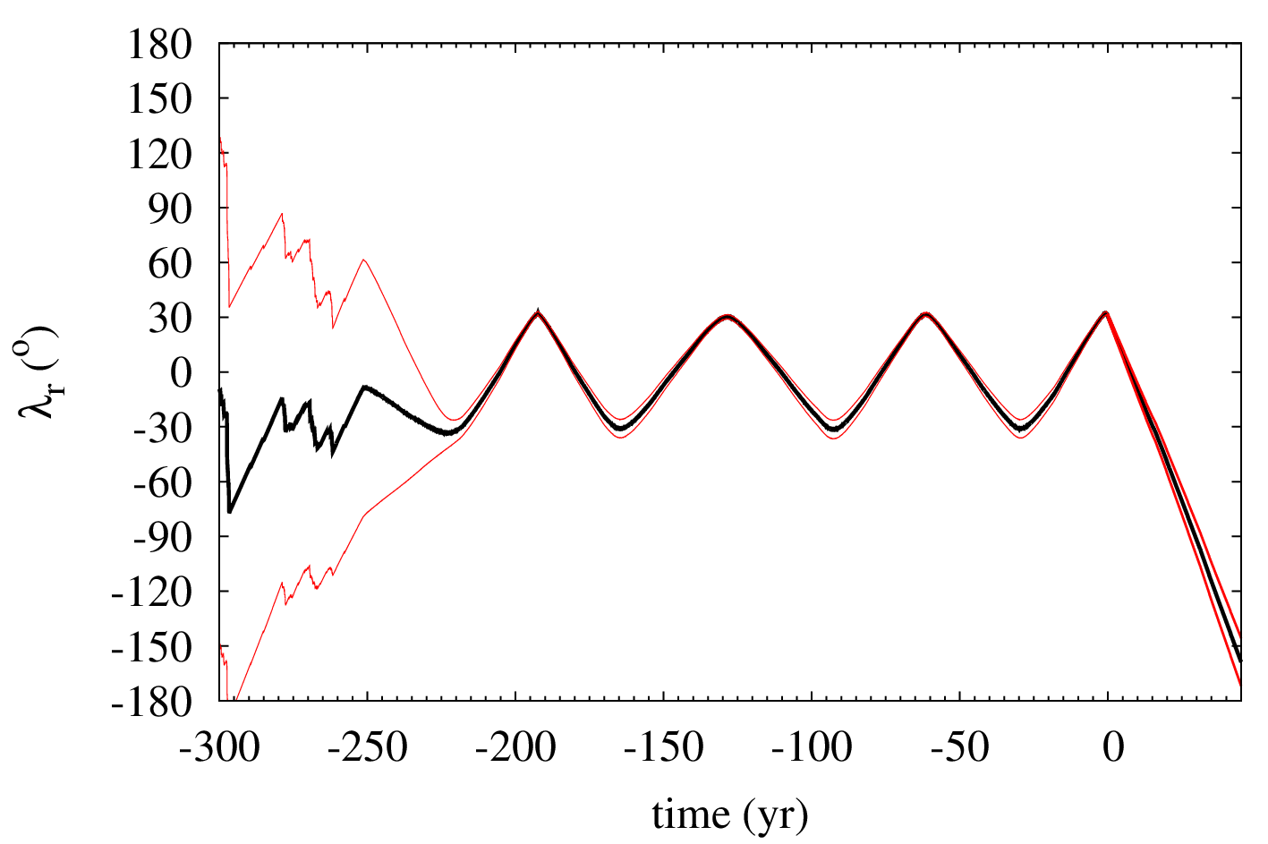
Fig. 1, top panel, shows that, prior to its close encounter with our planet on 2017 March 23, 2017 FZ2 was a quasi-satellite of the Earth with a period close to 60 yr as the value of the resonant angle was librating about zero with an amplitude of nearly 30°. The bottom panel in Fig. 1 only displays the time interval (250, 1) yr for clarity and shows complex, drifting yearly loops (the annual epicycles) as seen in a frame of reference centred at the Sun and rotating with the Earth. This result —for the time interval (225, 50) yr— is statistically robust as it is common to all the control orbits (over 103) investigated in this work. Extensive calculations (see below) show that the orbital evolution of this NEA is highly sensitive to initial conditions, much more than for any other previously documented quasi-satellite of our planet. A very chaotic orbit implies that it will be difficult to reconstruct its past dynamical evolution or make reliable predictions about its future behaviour beyond a few hundred years.

When observed from the ground, a quasi-satellite of the Earth traces an analemma in the sky (de la Fuente Marcos & de la Fuente Marcos 2016e,f).99 9 There is an error in terms of quoted units in figs 1 and 2 of de la Fuente Marcos & de la Fuente Marcos (2016e), and figs 2 and 3 of de la Fuente Marcos & de la Fuente Marcos (2016f), the right ascension is measured in hours not degrees in those figures. Fig. 2 shows ten loops of the analemmatic curve described by 2017 FZ2 (in red, nominal orbit) that is the result from the interplay between the tilt of the rotational axis of the Earth and the properties of the orbit of the quasi-satellite. Due to its significant eccentricity but low orbital inclination, its apparent motion traces a very distorted teardrop. Non-quasi-satellite co-orbitals do not trace analemmatic loops as seen from the Earth (see the blue curve in Fig. 2 that corresponds to 2017 DR109, an Earth’s co-orbital that follows a horseshoe-type path).

Consequently, 2017 FZ2 joins the list of quasi-satellites of our planet that already includes (164207) 2004 GU9 (Connors et al. 2004; Mikkola et al. 2006; Wajer 2010), (277810) 2006 FV35 (Wiegert et al. 2008; Wajer 2010), 2013 LX28 (Connors 2014), 2014 OL339 (de la Fuente Marcos & de la Fuente Marcos 2014, 2016c) and (469219) 2016 HO3 (de la Fuente Marcos & de la Fuente Marcos 2016f). Although it was the smallest known member of the quasi-satellite dynamical class —independent of the host planet and significantly smaller than the previous record holder, 469219, that has = 24.2 mag— it is no longer a member of this category; our calculations indicate that, after its most recent close flyby with our planet, it has become a non-resonant NEA.
The quasi-satellite resonant state —as the one experienced by 2017 FZ2 and the other five objects pointed out above--- was first described theoretically by Jackson (1913), but without the use of modern terminology. The energy balance associated with it was studied by Hénon (1969), who called the objects engaged in this unusual resonant behaviour ‘retrograde satellites’. However, such objects are not true satellites because they are not gravitationally bound to a host (i.e. have positive planetocentric energy). The term ‘quasi-satellite’ itself was first used in its present sense by Mikkola & Innanen (1997). Although the first quasi-satellite (of Jupiter) may have been identified (and lost) in 1973 (Chebotarev 1974),1010 10 Originally published in Russian, Astron. Zh., 50, 1071-1075 (1973 September–October). the first bona fide quasi-satellite (of Venus in this case), 2002 VE68, was documented by Mikkola et al. (2004). A modern theory of quasi-satellites has been developed in the papers by Mikkola et al. (2006), Sidorenko et al. (2014) and Pousse, Robutel & Vienne (2017). A recent review of confirmed quasi-satellites has been presented by de la Fuente Marcos & de la Fuente Marcos (2016e).
Fig. 1 shows that the most recent quasi-satellite episode of 2017 FZ2 started nearly 275 yr ago (but see below) and ended after a close encounter with the Earth on 2017 March 23. The past and future orbital evolution of this object as described by its nominal orbit in Table 1, left-hand column, is shown in Fig. 3, central panels; the evolution of two representative control orbits based on the nominal solution but adding (+) or subtracting () six times the corresponding uncertainty from each orbital element (all the six parameters) in Table 1, left-hand column, and labelled as ‘’ are displayed as well (right-hand and left-hand panels, respectively). These two examples of orbit evolution using initial conditions that are most different from those associated with the nominal orbit are not meant to show how wide the dispersion of the various parameters could be as they change over time; the statistical effect of the uncertainties will be studied later.
Figs 1 and 3 show that prior to its most recent flyby with our planet this NEA was an Aten asteroid (now it is an Apollo) following a moderately eccentric orbit, = 0.26, with low inclination, = 171, that kept the motion of this minor body confined between the orbits of Venus and Mars as it experienced close approaches to both Venus and the Earth (A- and H-panels). These two planets are the main direct perturbers of 2017 FZ2 —although Jupiter drives the precession of the nodes (see e.g. Wiegert, Innanen & Mikkola 1998). For this reason, the dynamical context of this NEA is rather different from that of the recently identified Earth’s quasi-satellite 469219 (de la Fuente Marcos & de la Fuente Marcos 2016f). The geocentric distance during the closest approaches shown in Fig. 3, A-panels, is often lower than the one presented in the figure due to its limited time resolution (a data output interval of 36.5 d was used for these calculations); for example, our (higher time resolution) calculations show that on 2017 March 23 the minimum distance between 2017 FZ2 and our planet was about 0.0045 au although Fig. 3, central A-panel, shows a value well above the Hill radius of the Earth, 0.0098 au, during the encounter.

Fig. 3 shows that 2017 FZ2 experienced brief quasi-satellite engagements with our planet in the past and it will return as Earth’s co-orbital in the future (C-panels); it may remain inside or close to the neighbourhood of Earth’s co-orbital zone for 20 kyr and possibly more although its orbital evolution is very chaotic (see below). The value of the Kozai-Lidov parameter (Kozai 1962; Lidov 1962) remains fairly constant (B-panels). In our case, oscillation of the argument of perihelion is observed for a certain period of time (Fig. 3) at = 270° (left-hand G-panels); libration about 180° has also been observed for other control orbits, but it is not shown here. When oscillates about 180° the NEA reaches perihelion while approaching the descending node; when librates about 270° (90°), aphelion always occurs away from the orbital plane of the Earth (and perihelion away from Venus). Some of these episodes correspond to domain III evolution as described in Namouni (1999), i.e. horseshoe-retrograde satellite orbit transitions and librations. This behaviour is also observed for 469219 (de la Fuente Marcos & de la Fuente Marcos 2016f) and other Earth’s co-orbitals or near co-orbitals (de la Fuente Marcos & de la Fuente Marcos 2015b, 2016a,b).

The current orbital solution for 2017 FZ2 is not as good as that of 469219, the fifth quasi-satellite of our planet, which has a data-arc spanning 13.19 yr; in any case, the overall evolution of 2017 FZ2 is significantly more chaotic as it is subjected to the direct perturbation of Venus and the Earth–Moon system. The combination of relatively poor orbital determination and strong direct planetary perturbations makes it difficult to predict the dynamical status of this object beyond a few centuries. Following the approach detailed in de la Fuente Marcos & de la Fuente Marcos (2015d), we have applied the Monte Carlo using the Covariance Matrix (MCCM) method to investigate the impact of the uncertainty in the orbit of 2017 FZ2 on predictions of its past and future evolution. Here and elsewhere in this paper, covariance matrices have been obtained from JPL’s horizons.
Fig. 4 shows results for 250 control orbits. Its future evolution is rather uncertain, which is typical of minor bodies with a perhaps non-negligible probability of colliding with our planet during the next century or so —as pointed out above, an impact was thought to be possible in 2101–2104 and the dispersion grows very significantly after that. In the computation of this set of control orbits (their orbital elements), the Box-Muller method (Box & Muller 1958; Press et al. 2007) has been used to generate random numbers according to the standard normal distribution with mean 0 and standard deviation 1 (for additional details, see de la Fuente Marcos & de la Fuente Marcos 2015d, 2016f). Our calculations show that the orbit of 2017 FZ2 is inherently very unstable due to its close planetary flybys and has a Lyapunov time —or characteristic time-scale for exponential divergence of integrated orbits that start arbitrarily close to each other— of the order of 102 yr. Such short values of the Lyapunov time are typical of planet-crossing co-orbitals (see e.g. Wiegert et al. 1998). Fig. 5 clearly shows how this circumstance affects the value of the resonant angle and the quasi-satellite nature of 2017 FZ2 (compare with Fig. 1, top panel).
Asteroid 2017 FZ2 will reach its next visibility window for observations from the ground starting in February 2018. From February 27 to March 18, it will be observable at an apparent visual magnitude cruising from right ascension 10h to 8h and declination +1° to +14°. Unfortunately, the Moon will interfere with any planned observations until March 10. This will be the best opportunity to gather spectroscopy of this object for the foreseeable future.
About 20 days before the discovery of 2017 FZ2, another small NEA, 2017 DR109, had been found following an orbit similar to that of 2017 FZ2.1111 11 http://www.minorplanetcenter.net/mpec/K17/K17E31.html The new minor body was observed by D. C. Fuls with the 0.68-m Schmidt camera of the Catalina Sky Survey at a visual apparent magnitude of 19.6 (Fuls et al. 2017). It is also a possible co-orbital of our planet, 0.0011 au, but smaller (9–20 m) than 2017 FZ2. Its current orbital solution is not as robust as that of 2017 FZ2 —see Table 1, central column— but it is good enough to arrive to solid conclusions regarding its current dynamical status, in the neighbourhood of . Fig. 6 shows the behaviour of the resonant angle of 2017 DR109 during the time interval (75, 75) yr; it is indeed a co-orbital and follows a horseshoe orbit with respect to our planet. Fig. 7 indicates that the orbital evolution of this object is nearly as chaotic as that of 2017 FZ2. Although it may remain inside or in the neighbourhood of Earth’s co-orbital zone for many thousands of years (see D-panels), it switches between the various co-orbital states (quasi-satellite, Trojan or horseshoe) and hybrids of them multiple times within the time interval displayed (see C-panels). Many of the dynamical aspects discussed regarding 2017 FZ2 are also present in Fig. 6. As for its next window of visibility, from 2018 February 23 to March 6 it will have an apparent visual magnitude , moving from right ascension 0h to 9h and declination +60° to +10°, but the Moon will interfere with the observations during this period. In general, objects following horseshoe-type paths with respect to the Earth can be observed favourably only for a few consecutive years (often less than a decade), remaining at low solar elongations —and beyond reach of ground-based telescopes— for many decades afterwards.


3 Are there too many of them?
The discovery of two small NEAs moving in rather similar orbits within 20 days of each other hints at the possible existence of a dynamical grouping as the past and future orbital evolution of both objects also bears some resemblance. In order to search for additional NEAs that may be following paths consistent with those of 2017 DR109 and 2017 FZ2, we use the D-criteria of Southworth & Hawkins (1963), , Lindblad & Southworth (1971), (in the form of equation 1 in Lindblad 1994 or equation 1 in Foglia & Masi 2004), Drummond (1981), , and the from Valsecchi, Jopek & Froeschlé (1999). These criteria are customarily applied using proper orbital elements not osculating Keplerian orbital elements like those in Table 1 (see e.g. Milani 1993, 1995; Milani & Knežević 1994; Knežević & Milani 2000; Milani et al. 2014, 2017).
Unfortunately, our exploration of the orbital evolution of 2017 DR109 and 2017 FZ2 in Section 2 indicates that, due to their short Lyapunov times, it may not be possible to estimate meaningful proper orbital elements for objects moving in such chaotic orbits. Proper elements are expected to behave as quasi-integrals of the motion, and are often computed as the mean semimajor axis, eccentricity and inclination from a numerical simulation over a long timespan; when close planetary encounters are at work, no relevant timespan can lead to parameters that remain basically unchanged. Although the dynamical context associated with these objects makes any exploration of their possible past connections difficult, a representative set of orbits of a given pair with low values of the D-criteria could be integrated to investigate whether their orbital evolution over a reasonable amount of time is also similar or not, confirming or disproving any indirect indication given by the values of the D-criteria based on osculating Keplerian orbital elements. Such an approach will be tested here.
3.1 The evidence
Table 2, top section, shows various orbital parameters and the values of the -criteria for objects with and with respect to 2017 FZ2 as described by its nominal orbit in Table 1, left-hand column. Unfortunately, the closest dynamical relatives of 2017 FZ2 are also small NEAs with poor orbital determinations, 2009 HE60 and 2012 VZ19. There are however in Table 2, top section, some relatively large NEAs with well-constrained orbital solutions, (488490) 2000 AF205 and (54509) YORP 2000 PH5. Asteroid 488490 is considered as an accessible NEA suitable for sample return missions (Christou 2003; Sears, Scheeres & Binzel 2003). Besides YORP, 2017 DR109 and 2017 FZ2, two other objects, 2009 HE60 and 2015 YA, are also confined within Earth’s co-orbital zone. Asteroid 2015 YA follows an asymmetric horseshoe trajectory (a hybrid of quasi-satellite and horseshoe that may evolve into a pure quasi-satellite state or a plain horseshoe one within the next century or so) with respect to the Earth, but it may not stay as Earth co-orbital companion for long due to the very chaotic nature of its orbital evolution (de la Fuente Marcos & de la Fuente Marcos 2016b); its orbit determination is as reliable as that of 2017 DR109 and it is in need of improvement as well.
| Asteroid | (au) | (°) | (°) | (°) | (yr) | (au) | (au) | arc (d) | (mag) | MOID (au) | ||||||
| 2009 HE60 | 0.99581 | 0.26487 | 1.58478 | 229.00798 | 219.87710 | 0.99 | 0.7321 | 1.2596 | 19 | 5 | 25.6 | 0.01544 | 0.5234 | 0.0100 | 0.2392 | 0.0209 |
| 2012 VZ19 | 0.98250 | 0.25406 | 1.24739 | 57.95044 | 221.44994 | 0.97 | 0.7329 | 1.2321 | 14 | 2 | 25.6 | 0.01111 | 0.0585 | 0.0163 | 0.0274 | 0.0435 |
| 488490 | 1.03408 | 0.27683 | 2.40837 | 220.06654 | 127.35081 | 1.05 | 0.7478 | 1.3204 | 157 | 6339 | 21.7 | 0.01818 | 0.2768 | 0.0178 | 0.0954 | 0.0403 |
| 2017 BU | 1.01959 | 0.25118 | 1.50522 | 75.57533 | 159.29112 | 1.03 | 0.7635 | 1.2757 | 59 | 14 | 25.1 | 0.02293 | 0.2295 | 0.0263 | 0.0804 | 0.0339 |
| 2015 YA | 0.99617 | 0.27938 | 1.61922 | 255.23303 | 83.61803 | 0.99 | 0.7179 | 1.2745 | 50 | 5 | 27.4 | 0.00349 | 0.2449 | 0.0281 | 0.0865 | 0.0310 |
| 2008 UB95 | 0.98970 | 0.26862 | 3.23715 | 21.96038 | 253.33450 | 0.98 | 0.7238 | 1.2556 | 58 | 363 | 24.7 | 0.00034 | 0.1024 | 0.0307 | 0.0361 | 0.0364 |
| 2016 JA | 1.01323 | 0.26845 | 0.05793 | 358.40711 | 112.58731 | 1.02 | 0.7412 | 1.2852 | 46 | 10 | 27.6 | 0.00017 | 0.5331 | 0.0309 | 0.2590 | 0.0098 |
| 2017 DR109 | 1.00064 | 0.24139 | 3.05996 | 341.31106 | 72.09400 | 1.00 | 0.7591 | 1.2422 | 29 | 5 | 27.6 | 0.00619 | 0.4612 | 0.0362 | 0.1861 | 0.0199 |
| 2012 BD14 | 1.01758 | 0.24045 | 1.53557 | 292.14513 | 293.67664 | 1.03 | 0.7729 | 1.2623 | 61 | 10 | 26.5 | 0.00795 | 0.2610 | 0.0398 | 0.1001 | 0.0421 |
| YORP | 1.00622 | 0.23022 | 1.59931 | 278.28130 | 278.86596 | 1.01 | 0.7746 | 1.2379 | 550 | 1826 | 22.7 | 0.00277 | 0.3526 | 0.0477 | 0.1426 | 0.0391 |
| 2000 QX69 | 1.01012 | 0.27146 | 4.57402 | 150.13180 | 74.18700 | 1.02 | 0.7359 | 1.2843 | 31 | 5 | 24.2 | 0.00020 | 0.2812 | 0.0491 | 0.0949 | 0.0175 |
| 2014 NZ64 | 1.03678 | 0.27343 | 4.49454 | 162.44887 | 273.58758 | 1.06 | 0.7533 | 1.3203 | 42 | 1046 | 22.8 | 0.00923 | 0.5218 | 0.0493 | 0.2250 | 0.0434 |
| with YORP | ||||||||||||||||
| 2012 BD14 | 1.01758 | 0.24045 | 1.53557 | 292.14513 | 293.67664 | 1.03 | 0.7729 | 1.2623 | 61 | 10 | 26.5 | 0.00795 | 0.1172 | 0.0104 | 0.0434 | 0.0199 |
| 2017 BU | 1.01959 | 0.25118 | 1.50522 | 75.57533 | 159.29112 | 1.03 | 0.7635 | 1.2757 | 59 | 14 | 25.1 | 0.02293 | 0.1661 | 0.0238 | 0.0692 | 0.0255 |
| 2017 DR109 | 1.00064 | 0.24139 | 3.05996 | 341.31106 | 72.09400 | 1.00 | 0.7591 | 1.2422 | 29 | 5 | 27.6 | 0.00619 | 0.4512 | 0.0318 | 0.1907 | 0.0247 |
| 2010 FN | 0.98958 | 0.21100 | 0.12365 | 161.55336 | 126.06353 | 0.98 | 0.7807 | 1.1984 | 31 | 4 | 26.6 | 0.00082 | 0.3152 | 0.0327 | 0.1196 | 0.0350 |
| 2002 VX91 | 0.98400 | 0.20127 | 2.34170 | 216.42578 | 78.74582 | 0.98 | 0.7859 | 1.1820 | 45 | 1942 | 24.3 | 0.00180 | 0.3294 | 0.0337 | 0.1360 | 0.0481 |
| 471984 | 1.02619 | 0.22570 | 3.35738 | 49.72365 | 117.40597 | 1.04 | 0.7946 | 1.2578 | 115 | 1020 | 22.7 | 0.02350 | 0.1441 | 0.0369 | 0.0488 | 0.0405 |
| 2007 WU3 | 1.01129 | 0.20401 | 2.39332 | 177.68825 | 351.97450 | 1.02 | 0.8050 | 1.2176 | 37 | 3164 | 23.8 | 0.04015 | 0.1232 | 0.0425 | 0.0736 | 0.0351 |
| 2009 BK2 | 1.01251 | 0.21259 | 3.55344 | 126.08145 | 121.52628 | 1.02 | 0.7973 | 1.2278 | 27 | 13 | 25.3 | 0.02604 | 0.2102 | 0.0446 | 0.0804 | 0.0227 |
| 2011 OJ45 | 1.01688 | 0.20367 | 0.74918 | 288.97227 | 135.40425 | 1.03 | 0.8098 | 1.2240 | 21 | 17 | 26.0 | 0.00755 | 0.4003 | 0.0465 | 0.1728 | 0.0500 |
| 2017 FZ2 | 1.00714 | 0.26406 | 1.81167 | 185.86918 | 100.32304 | 1.01 | 0.7412 | 1.2731 | 152 | 8 | 26.7 | 0.00139 | 0.3525 | 0.0477 | 0.1426 | 0.0391 |

Although the quality of the orbital determination of 2009 HE60 (Gibbs et al. 2009) is inferior to those of 2015 YA, 2017 DR109 or 2017 FZ2, our simulations show that this NEA is currently engaged in a brief quasi-satellite episode with our planet that started nearly 70 yr ago and will end in about 15 yr from now, to become a regular horseshoe librator for over 103 yr. Fig. 8, top panel, shows the evolution of the value of ; the bottom panel displays the path followed by 2009 HE60 in a frame of reference centred at the Sun and rotating with our planet, projected on to the ecliptic plane. Fig. 2 shows ten loops of the analemmatic curve described by 2009 HE60 (in green). We therefore confirm that 2009 HE60 is a robust candidate to being a current quasi-satellite of our planet. We speak of a candidate because its orbital solution is in need of some improvement; unfortunately, it has not been observed since 2009 April 29. Its next window of visibility spans from 2018 May 29 to June 9, when it will have an apparent visual magnitude , moving from right ascension 17h to 16h and declination 20° to 18°, but the Moon will interfere with the observations during most of this period. In any case, our planet appears to be second to none regarding the number of known quasi-satellites (see the review by de la Fuente Marcos & de la Fuente Marcos 2016e).
The presence of YORP among the list of candidates to being dynamical relatives of 2017 FZ2 in Table 2, top section, makes one wonder whether some of those small NEAs may be the result of mass shedding from YORP itself or a putative larger object that produced YORP. The data show that 2012 BD14 appears to follow an orbit akin to that of YORP. Table 2, bottom section, explores the presence of NEAs moving in YORP-like orbits (the nominal orbit of YORP is given in Table 1, right-hand column). The orbital similarity between YORP and 2012 BD14 is confirmed; another relatively large NEA with good orbital determination, (471984) 2013 UE3, is also uncovered. The sample of known NEAs moving in YORP-like orbits comprises a few objects with probable sizes larger than 100 m and several more down to the meteoroid size (a few metres). Some or all of them could be trapped in a web of overlapping mean-motion and secular resonances as described by de la Fuente Marcos & de la Fuente Marcos (2016d), but the very chaotic nature of this type of orbits subjected to the recurrent direct perturbations of Venus and the Earth–Moon system could favour an alternative scenario where some of these objects may have a past physical relationship. If some of these NEAs had a common genetic origin, one may expect that their dynamical evolution back in time kept them within a relatively small volume of the orbital parameter space.
Fig. 9 shows a number of backwards integrations for 10 000 yr corresponding to the nominal orbits of representative NEAs in Table 2. The points show the current parameters of the 19 different objects in Table 2. As this figure uses only nominal orbits and some of the 19 NEAs have poor orbit determinations, the purpose of this plot is simply act as a guide to the reader, not to provide an extensive exploration of the backwards dynamical evolution of these objects, which is out of the scope of this paper. In general, the backwards time evolution of these objects seems to keep them clustered within a relatively small region. Some pairs follow unusually similar tracks, for example YORP and 2012 BD14 or 471984 and 2007 WU3. In principle, it is difficult to conclude that the present-day orbits followed by some of these objects could be alike due to chance alone. But how often do NEAs end up and remain on an orbit within this region of the orbital parameter space?

3.2 The expectations
In order to provide a statistically robust answer to the question asked in the previous section, we use the list of near-Earth objects (NEOs) currently catalogued (as of 2017 July 20, 16 498 objects, 16 323 NEAs) by JPL’s Solar System Dynamics Group (SSDG) Small-Body Database (SBDB),1212 12 http://ssd.jpl.nasa.gov/sbdb.cgi concurrently with the NEOSSat-1.0 orbit model developed by Greenstreet, Ngo & Gladman (2012) and the newer one developed within the framework of the Near-Earth Object Population Observation Program (NEOPOP) and described by Granvik et al. (2013a,b) and Bottke et al. (2014), which is intended to be a state-of-the-art replacement for a widely used model described by Bottke et al. (2000, 2002). We use data from these two NEO models because such synthetic data do not contain any genetically related objects and they are free from the observational biases and selection effects that affect the actual data. These two features are critical in order to decide whether some of the NEAs in Table 2 may have had a physical relationship in the past or not.
The data from JPL’s SSDG SBDB (see Fig. 10, left-hand panels)1313 13 In this and subsequent histograms, the bin size has been computed using the Freedman-Diaconis rule (Freedman & Diaconis 1981), i.e. , where IQR is the interquartile range and is the number of data points. show that the probability of finding a NEA within Earth’s co-orbital zone is 0.00250.00041414 14 The uncertainty has been computed assuming Poissonian statistics, , see e.g. Wall & Jenkins (2012). (40 objects out of 16 323, but they may or may not be trapped in the 1:1 mean-motion resonance with our planet) and that the probability of finding a NEA following a YORP-like orbit —in other words, and with respect to YORP— is 0.000670.000251515 15 As before, we adopt Poissonian statistics to compute the uncertainty —applying the approximation given by Gehrels (1986) when , . (11 objects out of 16 323). These are of course biased numbers, but how do they compare with unbiased theoretical expectations?


A quantitative answer to this question can be found looking at the predictions made by a scientifically validated NEO model. For this task, we have used first the codes described in Greenstreet et al. (2012)1616 16 http://www.phas.ubc.ca/%7Esarahg/n1model/ with the same standard input parameters to generate sets of orbital elements including 16 498 virtual objects. The NEOSSat-1.0 orbit model was originally applied to compute the number of NEOs with mag (or a diameter of about 1 km) in each dynamical class —Vatiras, Atiras, Atens, Apollos and Amors. It can be argued that only about 6.4 per cent of known NEOs have mag, but if we assume that the size and orbital elements of asteroids are uncorrelated we can still use the NEOSSat-1.0 orbit model to compute reliable theoretical probabilities —this customary assumption has been contested by e.g. Bottke et al. (2014) and it is not used by the NEOPOP model. Fig. 10, central panels, shows a typical outcome from this NEO model. When we compare left-hand and central panels in Fig. 10, we observe that the two distributions are quite different in terms of the values of the orbital inclination. There is also a significant excess of synthetic NEOs with values of the semimajor axis close to 2.5 au that corresponds to minor bodies escaping the main asteroid belt through the 3:1 mean-motion resonance with Jupiter; the Alinda family of asteroids are held by this resonance (see e.g. Simonenko, Sherbaum & Kruchinenko 1979; Murray & Fox 1984).
The NEOSSat-1.0 model predicts that the probability of finding a NEO within Earth’s co-orbital zone is 0.00280.0003 and that of a NEO following a YORP-like orbit is 0.000030.00003 (averages and standard deviations come from ten instances of the model using different seeds to generate random numbers). It is clear that the values of the theoretical and empirical probabilities of finding a NEO within Earth’s co-orbital zone are statistically consistent; therefore, our assumption of lack of correlation between size and orbital elements might be reasonably correct, at least within the context of this research. Surprisingly, the empirical probability of finding a NEA following a YORP-like orbit is significantly higher than the theoretical one, over 21 higher. While it can be argued that our approach is rather crude, it is difficult to explain such a large difference as an artefact when the probabilities of finding a co-orbital agree so well (but see below for a more detailed discussion).
The NEOSSat-1.0 model is not the most recent and highest-fidelity NEO model currently available but, how different are the estimates provided by a more up-to-date model like NEOPOP? The software implementing the NEOPOP model is publicly available1717 17 http://neo.ssa.esa.int/neo-population and the model has been successfully applied in several recent NEO studies (Granvik et al. 2016, 2017). It accurately reproduces the orbits of the known NEOs as well as their absolute magnitudes and albedos, i.e. size and orbital elements of NEOs are correlated in this framework. The model is calibrated from mag up to mag; as our knowledge of the NEO population with mag is assumed to be complete, known NEOs have been used for this range of absolute magnitudes. Fig. 10, right-hand panels, shows a typical outcome from this model. The synthetic, unbiased distributions are quite different from the real ones (left-hand panels). The excess of synthetic NEOs with values of the semimajor axis close to 2.5 au is less significant than that of the NEOSSat-1.0 model. Using the standard options of the NEOPOP model, the code produces 802 457 synthetic NEOs with mag. Out of this data pool, we select random permutations (only for mag, the ones with mag remain unchanged) of 16 498 objects to compute statistics or construct the histograms in Fig. 10, right-hand panels.
The NEOPOP model predicts that the probability of finding a NEO within Earth’s co-orbital zone is 0.00210.0004 and that of a NEO following a YORP-like orbit is 0.000024 (averages and standard deviations come from 25 instances of the model). These two values of the probability agree well with those derived from the NEOSSat-1.0 model. Therefore, the theoretical and empirical probabilities of finding a NEO within Earth’s co-orbital zone are statistically consistent, but the empirical one of finding a NEA following a YORP-like orbit is well above any of the theoretical ones. It could be argued that the theoretical and empirical probabilities of finding a co-orbital are equal by chance. In addition, known NEAs in YORP-like orbits are simply more numerous in relative terms because they tend to pass closer to our planet and in consequence are easier to discover as accidental targets of NEO surveys. Although these arguments have significant weight, one can also argue that all the known Earth co-orbitals are serendipitous discoveries that were found as a result of having experienced very close encounters with our planet.
Regarding the issue of observed and predicted absolute magnitudes, let us focus only on NEOs, real or synthetic, with mag. The probabilities given by the NEOPOP model are the values already cited. The data from JPL’s SSDG SBDB give a value of 0.00210.0004 (27 out of 12736 objects) for the probability of finding a NEA with mag within Earth’s co-orbital zone, which is a perfect match for the theoretical estimate from the NEOPOP model. As for YORP-like orbits with mag, the empirical value of the probability is 0.0003 (4 out of 12736 objects). Even if we take into account the values of , the theoretical value of the probability of observing a YORP-like orbit is significantly below the empirical value. In addition, the NEOPOP model predicts no NEOs with mag moving in YORP-like orbits but there are two known, YORP and 471984. It is true that the evidence is based on small samples but one tantalizing albeit somewhat speculative possibility is that some of these objects have been produced in situ via fragmentation events, i.e. they are direct descendants of minor bodies that were already moving in YORP-like orbits.
On the other hand, the synthetic data generated to estimate the theoretical values of the probabilities can be used together with the D-criteria to uncover unusual pairs among the NEAs in Table 2. The procedure is simple, each set of synthetic NEOs from NEOSSat-1.0 or NEOPOP comprises fully unrelated virtual objects. If we compute the D-criteria with respect to the real YORP (or 2017 FZ2) for all the virtual NEOs in a given set and perform a search looking for those with and , we can extract a sample of relevant unrelated (synthetic) NEAs and compute the expected average values and standard deviations of the D-criteria when no orbital correlation between pairs of objects is present in the data. These averages and dispersions can be used to estimate how unlikely (in orbital terms) the presence of a given pair of real objects is.
In order to evaluate statistically this likelihood, we compute the absolute value of the difference between the value of a certain D-criterion for a given pair of objects in Table 2 and the average value for uncorrelated virtual objects, then divide by the dispersion found from the synthetic data. If the estimator gives a value close to or higher than 2 we may assume that the pair of objects could be unusual (an outlier, in statistical parlance) within the fully unrelated pairs scenario and perform additional analyses. We have carried out this investigation and the estimator discussed gives values around 1 for all the tested pairs with one single exception, the pair YORP–2012 BD14 that gives values of the estimator in the range 2–3 for all the D-criteria.
A simple scenario that may explain the observed excess or even the presence of the unusual pair YORP–2012 BD14 is in-situ production of NEAs moving in YORP-like orbits either as a result of mass shedding from YORP itself (or any other relatively large NEA in this group) or a putative bigger object that produced YORP (or any other of the larger objects in Table 2). However, it is not just the size of this population that matters: we also have the issue of its stability and how many concurrent resonant objects should be observed in these orbits at a given time. Finding answers to these questions requires the analysis of relevant -body simulations. Given the chaotic nature of these orbits, relatively short calculations should suffice to arrive to robust conclusions.
In order to explore the stability and resonant properties of YORP-like orbits, we have performed 20 000 numerical experiments using the same software and physical model considered in the previous section and orbits for the virtual NEOs uniformly distributed (i.e we do not make any assumptions on the origin, natural versus artificial, of the virtual objects) within the ranges au, , °, °, and °, i.e. consistent with having and with respect to YORP. After an integration of 2 000 yr forward in time we obtain Figs 11 and 12. For each simulated particle we compute the average value and the standard deviation of the resonant angle in the usual way (see e.g. Wall & Jenkins 2012); the standard deviation of a non-resonant angle is 103923. In Fig. 11, nearly 66 per cent of the virtual NEOs do not exhibit any sign of resonant behaviour during the simulation, 0.7 per cent are quasi-satellites, nearly 1.8 per cent are Trojans, and 5.6 per cent move in horseshoe orbits, the remaining 25.9 per cent follow elementary or compound 1:1 resonant states for at least some fraction of the simulated time. Fig. 12 shows that the most stable configurations are invariably characterized by very long synodic periods (i.e. 1 au) and lower .
From Table 2, bottom section, and results in Sections 2 and 3, as well as results from the literature, we have at least three objects held by the 1:1 mean-motion resonance with our planet out of 11 listed NEAs. In other words, over 27 per cent of all the objects moving in YORP-like orbits exhibit signs of resonant behaviour when the theoretical expectation in the framework of a fully random scenario is about 34 per cent. This result can be regarded as another piece of evidence in support of our previous interpretation because the orbital distribution of NEAs is not expected to be random (in the sense of uniform), see Fig. 10, and real NEAs are not supposed to have formed in these peculiar orbits, but come from the main asteroid belt. In addition we have found one quasi-satellite (2017 FZ2) out of 11 NEAs in Table 2, bottom section, and two NEAs moving in horseshoe-type paths (YORP and 2017 DR109), i.e. a quasi-satellite probability of about 9 per cent when the random scenario predicts 0.7 per cent and a horseshoe probability of about 18 per cent when the random scenario predicts 5.6 per cent.


The various aspects discussed above strongly suggest that some of the NEAs in Table 2 may form a dynamical grouping and perhaps have a genetic connection. Evidence for the presence of possible dynamical groupings among the co-orbital populations of our planet has been discussed in the case of NEAs moving in Earth-like orbits, the Arjunas (de la Fuente Marcos & de la Fuente Marcos 2015a), and also the group of objects following paths similar to those of 2015 SO2, (469219) 2016 HO3 and 2016 CO246 (de la Fuente Marcos & de la Fuente Marcos 2016a,f). However, the study by Schunová et al. (2012) could not find any statistically significant group of dynamically related NEAs among those known at the time, but it is also true that many objects in Table 2 have been discovered after the completion of that study.
4 Mutual close encounters: happening by chance or not?
If the excess of NEAs following YORP-like orbits is statistically significant, one would expect that some of the asteroid pairs under study had their orbits intersecting one another in the past and perhaps that their relative velocities were very low during such very close approaches. An exploration of this scenario requires the analysis of large sets of -body simulations backwards in time for each relevant pair, but in order to identify any results as statistically significant we must study first what happens in the case of a random population of virtual NEAs moving in YORP-like orbits. The statistical analysis of minimum approach distances and relative velocities between unrelated objects can help us distinguish between close encounters happening by chance and those resulting from an underlying dynamical (and perhaps physical) relationship.
Using a sample of 10 000 pairs of unrelated, virtual NEAs with orbits uniformly distributed within the ranges considered in the numerical experiments performed in the previous section, and integrated backwards in time for 2 000 yr, we have studied how is the distribution of relative velocities at minimum approach distance ( au, the first quartile is 0.0046 au and the average is 0.017 au) during mutual encounters. Given the fact that these NEAs are too small to change significantly their orbits due to their mutual gravitational attraction during close encounters, such a velocity distribution can be considered as a reasonably robust proxy for the representative collision velocity distribution for pairs of NEAs following YORP-like orbits. The results of this analysis may apply to both natural and artificial objects.


Fig. 13, left-hand panels, shows the distribution of relative velocities at minimum distance for pairs of virtual NEAs in YORP-like orbits like those in the numerical experiments performed in the previous section. The most likely encounter velocities are near the high velocity extreme, which is characteristic of encounters near perihelion where multiple encounter geometries are possible. The mean approach velocity falls in the low-probability dip between the high-probability peak at about 14 km s-1 (encounters at perihelion) and the secondary peak at about 3 km s-1 (encounters at aphelion). However, the closest approaches (at about 10 000 km from each other) are characterized by values of the relative velocity close to 13 km s-1 due to their relatively high eccentricity. The results in Fig. 13, left-hand panels, do not take into account predictions from the NEOPOP model and this may be seen as a weakness of our analysis. In order to explore possible systematic differences, we have completed an additional set of calculations using the actual synthetic orbits predicted by the NEOPOP model as input, but randomizing the values of and , then picking up pairs at random to compute the new set of simulations. The results of these calculations are shown in Fig. 13, central panels, and are quite similar to those in the left-hand panels. However, the ranges in the values of , and are slightly different. We have repeated the calculations using uniform orbital distributions, but for the ranges au, , and °; Fig. 13, right-hand panels, shows that the results are very much alike. Although no actual collisions have been observed during all these simulations, the velocity distribution in Fig. 13 is the one we seek as the mutual gravitational perturbation is negligible even during the closest mutual flybys.
Fig. 13 shows that the mean value of the velocity and its dispersion do not represent the distribution well. Collisions between these minor bodies yield higher probable collision velocities although high speed lowers the overall collision probability (the probability of experiencing an encounter closer than 30 000 km is of the order of 0.0002). However, impacts from meteoroids originated within this population on members of the same population happen at most probable velocities high enough to perhaps induce catastrophic disruption or at least partial destruction of the target as the impact kinetic energy goes as the square of the collision velocity. Our results closely resemble those obtained by Bottke et al. (1994) for the velocity distributions of colliding asteroids in the main asteroid belt.
YORP-induced catastrophic asteroid breakups can generate multiple small NEAs characterized by pair-wise velocity dispersions under 1 m s-1 and also clouds of dust as observed in the case of P/2013 R3 (Jewitt et al. 2017). Groups of objects moving initially along similar paths lose all dynamical coherence in a rather short time-scale (Pauls & Gladman 2005; Rubin & Matson 2008; Lai et al. 2014). This randomization is accelerated when recurrent close planetary encounters are possible. As the virtual NEAs used in our numerical experiments move in uncorrelated orbits, the results in Fig. 13 can be used to single out pairs of objects that exhibit some level of orbital coherence; this feature may signal a very recent (not more than a few thousand years ago) breakup event. The velocity distribution of any pair of unrelated NEAs following YORP-like orbits is expected to be strongly peaked towards the high end of the distribution in Fig. 13, i.e. yield a most probable collision velocity close to or higher than 13 km s-1. We have explored the velocity distributions of multiple pairs of objects in Table 2 using the same approach applied before and found that this is true for the vast majority of them. However, we have found two notable exceptions, the pairs (54509) YORP 2000 PH5–2012 BD14 and YORP–2007 WU3. The first one has a non-negligible probability of experiencing close encounters with relative velocities well under 1 km s-1, 0.0007. The second one has a most probable close approach velocity km s-1 —the probability of a value of the close approach velocity that low or lower is 0.77— well below the high-probability peak at 14 km s-1 in Fig. 13. The probability of having a close approach velocity km s-1 from Fig. 13 is 0.14.
Asteroid 2012 BD14 has a relatively good orbit (Holmes et al. 2012) as it has one radar Doppler observation, but lacks any additional data other than those derived from the available astrometry/photometry. Assuming similar composition, this Apollo asteroid must be as large as 2017 FZ2 (15–33 m). In order to compute the velocity distribution for the pair YORP–2012 BD14, we have performed an analysis analogous to that in Fig. 13 but using control orbits for both objects generated by applying the MCCM method as described above and integrating backwards for 1 000 yr. Fig. 14 shows that the most probable collision velocity in this case is 4 km s-1 and about 7 per cent of flybys have relative velocities close to or below 2 km s-1, but down to 336 m s-1. In addition, the probability of experiencing an encounter closer than 30 000 km is 0.0013, which is significantly higher than that of analogous encounters for random YORP-like orbits. In other words, it is possible to find control orbits —albeit with relatively low probability— of YORP and 2012 BD14, statistically compatible with the available observations, that place them very close to each other and moving at unusually low relative speed in the recent past. These approaches are observed at 0.75–0.9 au from the Sun, i.e. in the inmediate neighbourhood of Venus. Although outside the scope of this paper, it may be possible to find control orbits of these two objects that may lead to grazing encounters at velocities of a few m s-1 if a much larger sample of orbits is analysed (the current one consists of 3 000 virtual pairs). It is difficult to explain such a level of coherence in their recent past orbital evolution as due to chance causes; these two objects could be genetically related. Unfortunately, 2012 BD14 reached its most recent visibility window late in summer 2017, from August 25 to September 18, but this NEA will become virtually unobservable from the ground during the next few decades.

The case of YORP and 2007 WU3 (Gilmore et al. 2007; Bressi, Schwartz & Holvorcem 2015) is markedly different from the previous one and also from the bulk of pairs in Table 2, and deserves a more detailed consideration. A velocity distribution analysis similar to that in Fig. 13 but using control orbits for both objects generated by applying the covariance matrix methodology described before and integrating backwards in time for 2 000 yr (see Fig. 15) shows that the most probable (close to 80 per cent) collision speed in this case is km s-1 and over 20 per cent of encounters have relative velocities close to or below 2 km s-1. The velocity distribution is clearly bimodal with the most probable encounter velocities near the low-velocity extreme, which is typical of encounters near aphelion where a multiplicity of flyby geometries are possible. The mean approach velocity falls in the low-probability dip between the high-probability peak at about 2.3 km s-1 (encounters at aphelion) and the secondary peak at about 3.8 km s-1 (encounters at perihelion). However, the closest approaches (at about 19 000 km from each other) are characterized by values of the relative velocity close to 2.5 km s-1. In addition, the probability of experiencing an encounter closer than 30 000 km is 0.0007.
Although the orbital solutions of both objects are not as precise as those of widely accepted young genetic pairs —for example, 7343 Ockeghem (1992 GE2) and 154634 (2003 XX28) as studied by Duddy et al. (2012) or 87887 (2000 SS286) and 415992 (2002 AT49) as discussed by Žižka et al. (2016)— and their dynamical environment is far more chaotic, this unusual result hints at a possible physical connection between these two NEAs although perhaps the YORP mechanism was not involved in this case. The velocity distributions for asteroid families studied by Bottke et al. (1994) —see their figs 10a, 11a, 12a and 13a— clearly resemble what is observed in Fig. 15, in particular that of the Eos family (their fig 10a) which is non-Gaussian and bimodal with the most probable collisions occurring near the apses; the lowest encounter velocities are observed when their perihelia are aligned and the highest when they are anti-aligned. In the case of YORP and 2007 WU3, low-velocity encounters take place at about 1.22 au from the Sun and the high-velocity ones at 0.81 au. These two objects are no longer observable from the ground and they will remain at low solar elongation as observed from the Earth for many decades.

The Eos family is the third most populous in the main asteroid belt and is thought to be the result of a catastrophic collision (Hirayama 1918; Mothé-Diniz & Carvano 2005), although its long-term evolution is also driven by the YORP effect (Vokrouhlický et al. 2006); many of its members are of the K spectral type and others resemble the S-type (see e.g. Mothé-Diniz, Roig & Carvano 2005). Having a comparable short-term orbital evolution can be used to argue for a dynamical connection but not to claim a physical connection. Genetic pairs must also have a similar chemical composition that can be studied via visible or near-infrared spectroscopy. Gietzen & Lacy (2007) carried out near-infrared spectroscopic observations of YORP and concluded that it belongs to either of the silicaceous taxonomic classes S or V. Mueller (2007) has pointed out that a S-type classification would be in excellent agreement with data from the Spitzer Space Telescope. Asteroid 2007 WU3 may be of Sq or Q taxonomy according to preliminary results obtained by the NEOShield-2 collaboration (Dotto et al. 2015).1818 18 http://www.neoshield.eu/wp-content/uploads/NEOShield-2_D10.2_i1__Intermediate-observations-and-analysis-progress-report.pdf If YORP and 2007 WU3 are genetically related, their mutual short-term dynamical evolution suggests that they are the result of a catastrophic collision not the YORP effect. Such collisions are unusual, but not uncommon; asteroid (596) Scheila 1906 UA experienced a sub-critical impact in 2010 December by another main belt asteroid less than 100 m in diameter (Bodewits et al. 2011; Ishiguro et al. 2011; Jewitt et al. 2011; Moreno et al. 2011; Yang & Hsieh 2011; Bodewits, Vincent & Kelley 2014). In this case, the impact velocity was probably close to 5 km s-1 (Ishiguro et al. 2011).
5 Encounters with planets and other NEOs
In addition to experiencing close encounters with other objects moving in YORP-like orbits, Fig. 3 shows that these interesting minor bodies can undergo close encounters with Venus, the Earth and (rarely) Mars. Close encounters with members of the general NEO population are possible as well. The circumstances surrounding such encounters are explored statistically in this section.
5.1 Encountering other NEOs
We have already found that collisions between NEAs following YORP-like orbits are most likely happening at relative velocities close to 13 km s-1, but most NEAs are not moving in YORP-like orbits. Here, we study the most general case of a close encounter between a virtual NEA moving along a YORP-like trajectory and a member of the general NEO population. In order to explore properly the available orbital parameter space, our population of virtual general NEAs has values of the orbital elements uniformly distributed within the domain au (uniform in , not in ), , °, °, and °. Fig. 16 shows a velocity distribution that is very different from that in Fig. 13; instead of being nearly bimodal, it is clearly unimodal although the most likely value of the encounter velocity is similar to that in Fig. 13. About 90 per cent of encounters/collisions have characteristic relative velocities in excess of 7 km s-1 and about 55 per cent, above 15 km s-1. If one of the minor bodies discussed here experiences a collision with another small NEA, the impact speed will be probably high enough to disrupt the object, partially or fully, creating a group of genetically (both physically and dynamically) related bodies.

Fig. 17 shows the encounter velocity (colour coded) for the pairs in Fig. 16 as a function of the initial values of the orbital parameters —, and — of the general NEA. As NEAs with low values of and high values of are rare, very high-speed collisions are unlikely. Relatively low-speed collisions mostly involve NEAs moving in low-eccentricity, low-inclination orbits. The lowest velocities ( km s-1) have been found for au, , and ° which is precisely the volume of the orbital parameter space enclosing those NEAs following YORP-like orbits. As expected, very low-speed collisions are only possible among members of the same dynamical class (i.e. when they have very similar orbits).

The previous analysis is based on the wrong assumption that NEOs have values of the orbital elements uniformly distributed; Fig. 10 clearly shows that this is not the case. On the other hand, sampling uniformly can oversample high eccentricities and inclinations, which lead to higher encounter velocities. In order to obtain unbiased estimates, we have performed additional calculations using a population of synthetic NEOs from the NEOPOP model to obtain Figs 18 and 19. The most probable value of the relative velocity during encounters is 15 km s-1 and the most likely value of the semimajor axis of the orbits followed by NEOs experiencing flybys with NEAs following YORP-like orbits is 2.5 au. This more realistic analysis still shows that the most probable impact speed during a hypothetical collision between a general NEO and one object following a YORP-like orbit could be high enough to cause significant damage to both NEOs.


5.2 Encountering Venus
Tables 1 and 2, and Figs 3 and 7 show that minor bodies following YORP-like orbits have perihelion distances that place them in the neighbourhood of the orbit of Venus. This fact clears the way to potential close encounters with this planet as one of the nodes could be in the path of Venus (see Fig. 3, H-panels). In order to investigate this possibility, we have performed short integrations (50 yr) of virtual NEAs with orbits as those described in Section 3 and under the same conditions. We decided to use short integrations to minimize the effects on our results derived from the inherently chaotic orbital evolution of these objects. Out of all the experiments performed, we have focused on 25 000 cases where the minimum distance between the virtual NEA and Venus during the simulation reached values under 0.1 au. We have found that for this type of orbit, the probability of experiencing such close encounters with Venus is about 82.2 per cent (this value of the probability has been found dividing the number of experiments featuring encounters under 0.1 au by the total number of experiments performed). Our calculations show that nearly 2 per cent of YORP-like orbits can lead to encounters under one Hill radius of Venus (0.0067 au), about 0.03 per cent approach closer than 20 planetary radii and 0.01 per cent closer than 10 planetary radii.
Although relatively close encounters are frequent, the probability of placing the virtual NEA within the volume of space that could be occupied by putative natural satellites of Venus is rather small for these orbits. Outside 10 planetary radii, the velocity of the incoming body with respect to Venus during the closest encounters is in the range (5, 7) km s-1; inside 10 planetary radii the speed of the virtual NEA is significantly increased due to gravitational focusing by Venus. Fig. 20 shows that the distribution of relative velocities at minimum distance is far from symmetric and the peak of the distribution does not correspond to the typical values observed when the distance from Venus to the virtual NEA is the shortest possible. In principle, NEAs that experience close encounters with Venus (or the Earth) can suffer resurfacing events when large rocks are dislodged from the surface of the minor body. Our calculations indicate that this may be happening to NEAs following YORP-like orbits, but the chance of this happening is low during encounters with Venus —the probability of encounters under 10 Venus radii is just 0.01 per cent.

5.3 Encountering the Earth: evaluating the impact risk
Here, we use the same set of simulations analysed in the previous section to perform a risk impact assessment evaluating the probability that an object moving in a YORP-like orbit experiences a close encounter with our planet. We found that the probability of suffering a close encounter under 0.1 au with the Earth is about 74.8 per cent (from 20 000 experiments). Our calculations also show that over 10 per cent of YORP-like orbits can approach the Earth closer than one Hill radius (0.0098 au), about 0.14 per cent approach under 20 planetary radii and 0.05 per cent below 10 planetary radii. The overall upper limit for the impact probability with our planet could be which is higher than that with Venus.
Although the objects of interest here tend to approach Venus more frequently, when they approach our planet, they do it at a closer distance. In principle, the Earth could be more efficient in altering the orbits of these small bodies, but Fig. 21 shows that the most probable value of the relative velocity at closest approach is nearly 8 km s-1 with a Gaussian spread or standard deviation of 1.230 km s-1. This is higher than for flybys with Venus. Encounters at lower relative speed could be more effective at modifying the path of the perturbed minor body because it will spend more time under the influence of the perturber during the flyby. Taking into account that the values of the masses of Venus and the Earth are very close, the overall influence of both planets on the orbits of NEAs following YORP-like orbits could be fairly similar. In addition, close encounters can happen in sequence; i.e. an inbound NEO can experience a close flyby with our planet that may facilitate a subsequent close encounter with Venus or an outbound NEO can approach Venus at close range making a close flyby with the Earth possible immediately afterwards.

Figs 20 and 21 show that the most probable value of the relative velocity at closest approach is higher for close encounters with our planet than for flybys with Venus and one may find this counterintuitive because at 0.7 au Keplerian velocities are higher than at 1 au. However, for flybys near perihelion multiple encounter geometries are possible. The situation could be analogous to that of Amor asteroids (or Apollos with perihelion distances 1 au) encountering the Earth. Independent calculations by JPL’s horizons give a range of 4.94 to 11.64 km s-1 for the relative velocity during encounters between 2017 FZ2 and Venus during a time span of nearly 300 yr; in the case of encounters with the Earth it gives a range of 4.63 to 22.52 km s-1.
Several objects in Table 2 have very small values of their MOIDs with respect to the Earth, some as small as 30 000 km or under 5 Earth radii. NEAs moving in these orbits clearly pose a potential risk of impact with our planet. In addition to 2017 FZ2 (and its initially possible impact in 2101–2104), two other small NEAs in Table 2 have a non-negligible probability of colliding with our planet in the near future as computed by JPL’s Sentry System. Asteroid 2010 FN has an estimated impact probability of 0.0000039 for a possible collision in 2079--2116.1919 19 https://cneos.jpl.nasa.gov/sentry/details.html#?des=2010%20FN Asteroid 2016 JA has an impact probability of 0.000001 for a possible impact in 2064--2103.2020 20 https://cneos.jpl.nasa.gov/sentry/details.html#?des=2016%20JA
5.4 Encountering Mars
Calculations analogous to the ones described in the cases of Venus and the Earth show that although relatively distant encounters (0.1 au) between objects moving in YORP-like orbits and Mars are possible, the actual probability is about 0.6 per cent and we found no encounters under one Hill radius of Mars (0.0066 au). The velocity of these bodies relative to Mars at its smallest separation is in the interval (4, 5) km s-1 (see Fig. 22). The role played by Mars on the dynamical evolution of these minor bodies is clearly negligible.

6 Discussion
Asteroid 2017 FZ2 was, prior to its close encounter with the Earth on 2017 March 23, a quasi-satellite of our planet. It was the smallest detected so far ( mag) and also moved in the least inclined orbit (). This minor body is no longer trapped in the 1:1 mean-motion resonance with our planet, but it has been trapped in the past and it could be again in the future. Its orbit is highly chaotic and it was even suggested that this NEA may collide with our planet in the near future ( yr), but it is seen as of less potential concern because of its small size.
Although apparently insignificant, this small body has led us to uncover a larger set of NEAs that appears to be at least some sort of grouping of dynamical nature that perhaps includes several objects that may be genetically related. It is not possible to reach robust conclusions regarding a possible connection between them because there is no available spectroscopic information for the vast majority of these NEAs and their current orbital solutions are not yet sufficiently reliable. Most of these NEAs have few observations and/or have not been re-observed for many years; a few of them, (54509) YORP 2000 PH5 included, may remain out of reach of ground-based telescopes for many decades into the future.
Objects in YORP-like orbits2121 21 As pointed out above, and with respect to YORP or (see Table 2, bottom section) au, , °, °, and °. might be returning spacecraft, but their obvious excess makes this putative origin very unlikely. Although a number of items of space debris and working spacecraft (e.g. Rosetta, Gaia or Hayabusa 2) have been erroneously given minor body designations, their orbits tend to be comparatively less inclined and far less eccentric, and their absolute magnitudes closer to 30. In addition, any artificial interloper within the group of objects moving in YORP-like orbits would have been originally Venus-bound and there are not many of those; besides, artificial objects without proper mission control input tend to drift away from Earth’s co-orbital region rather quickly (see e.g. section 9 of de la Fuente Marcos & de la Fuente Marcos 2015b). They may be lunar ejecta, but our calculations suggest that these objects cannot remain in their orbits for a sufficiently long period of time, say for the last 100 000 yr. The only alternative locations for the origin of these bodies are either the asteroid belt or having been produced in situ (i.e. within Earth’s immediate neighbourhood) via YORP spin-up or any other mechanism able to generate fragments. Our analysis using the NEOSSat-1.0 and NEOPOP orbital models indicates that the known delivery routes from the asteroid belt to the YORP-like orbital realm might not be efficient enough to explain the high proportion of small NEAs currently moving in YORP-like orbits. The presence of several relatively large minor bodies, YORP included, and a rather numerous dynamical cohort of much smaller objects hints at a possible genetic relationship between several of the members of this group. Arguing for a genetic relationship requires both robust dynamical and compositional similarities. However, it is also entirely possible that the existence of observational biases may account, at least partially, for the observed excess.
Small NEAs could be the result of the YORP mechanism, but they may also be the by-product of collisions or the aftermath of tidal stripping events during low-velocity close encounters with the planets, in particular with the Earth (see e.g. Bottke & Melosh 1996a,b). Asteroids encountering the Earth (or Venus) with low relative velocity are good candidates for disruption because tidal splitting is more likely at low relative velocity. Objects following YORP-like orbits encounter the Earth preferentially with relative velocity in the range 6–8 km s-1 (the encounter statistics analysed in Section 5.3). Morbidelli et al. (2006) have shown that (see their fig. 2), when encountering the Earth at these low relative velocities, any fragment resulting from tidal stripping can become physically unbound in a relatively short time-scale, producing a pair of genetically related NEAs.
On the other hand, low-speed flybys, which are more sensitive to gravitational perturbations from our planet, tend to retain the coherence of the nodal distances for shorter time-scales and are more prone to generate a dynamical grouping or meteoroid stream after tidal disruption. Fig. 23 shows the behaviour of the nodal distances for a number of objects in Table 2 (also see H-panels in Figs 3 and 7). As the orbit determinations of 2009 HE60 and 2012 VZ19 are rather poor, Fig. 23 is only meant to be an example, not a numerically rigorous exploration of this important issue; in any case and although certain objects appear to exhibit some degree of (brief) nodal coherence, the evolution is often too chaotic to be able to arrive to any reliable conclusions. The pair-wise approach followed in Section 4 seems to be the only methodology capable of producing robust evidence, either in favour or against a possible dynamical relationship.

The picture that emerges from our extensive analysis is a rather complex one. YORP-induced rotational disruption may be behind the origin of some of the small bodies discussed in this paper (as it could be the case of the pair YORP–2012 BD14), but the fact that they also experience very close encounters with both Venus and our planet cannot be neglected. On the other hand, once fragments are produced either during planetary encounters or as a result of the YORP effect, these meteoroids can impact other objects moving along similar paths at relatively high velocities triggering additional fragmentations (perhaps the case of the pair YORP–2007 WU3) or even catastrophic disruptions leading to some type of cascading effect that can eventually increase the size of the population moving along these peculiar orbits and perhaps explain the observed excess. Subcatastrophic collisions and tidal encounters can also lead to further rotational disruptions. The dynamical environment found here is rather different from the one surrounding typical main-belt asteroid families; here, very close planetary encounters are possible in addition to the active role played by mean-motion and secular resonances that are also present in the main asteroid belt.
In this paper, we have not included the results of the Yarkovsky and YORP effects (see e.g. Bottke et al. 2006), but ignoring these effects has no relevant impact on our analysis, which is based on relatively short integrations, or our conclusions. Not including these non-gravitational forces in our integrations is justified by the fact that the largest predicted Yarkovsky drift rates are 10-7 au yr-1 (see e.g. Farnocchia et al. 2013) and also because the physical properties —such as rotation rate, albedo, bulk density, surface conductivity or emissivity— of most of the NEAs under study here are not yet known and without them, no reliable calculations can be attempted. The width of the co-orbital region of the Earth is about 0.012 au; at the highest predicted Yarkovsky drift rates, the characteristic time-scale to leak from the co-orbital region of our planet is equal to or longer than 120 000 yr that is much larger than the time-scales pertinent to this study —for an average value for the Yarkovsky drift of 10-9 au yr-1, the time-scale to abandon the region of interest reaches 12 Myr.
7 Conclusions
In this paper, we have studied the orbital evolution of the recently discovered NEA 2017 FZ2 and other, perhaps related, minor bodies. This research has been performed using -body simulations and statistical analyses. Our conclusions can be summarized as follows.
- (i)
Asteroid 2017 FZ2 was until very recently an Earth’s co-orbital, the sixth known quasi-satellite of our planet and the smallest by far. Its most recent quasi-satellite episode may have started over 225 yr ago and certainly ended after a close encounter with the Earth on 2017 March 23.
- (ii)
Extensive -body simulations show that the orbit of 2017 FZ2 is very unstable, with a Lyapunov time of the order of 100 yr.
- (iii)
Our orbital analysis shows that 2017 FZ2 is a suitable candidate for being observed spectroscopically as it will remain relatively well positioned with respect to our planet during its next visit in 2018.
- (iv)
Over a dozen other NEAs move in orbits similar to that of 2017 FZ2, the largest named being (54509) YORP 2000 PH5. Among these objects, we have identified two present-day co-orbitals of the Earth not previously documented in the literature: 2017 DR109 follows a path of the horseshoe type and 2009 HE60 is confirmed as a strong candidate to being a quasi-satellite.
- (v)
We find an apparent excess of small bodies moving in orbits akin to that of YORP that amounts to an over twentyfold increase with respect to predictions from two different orbital models and we argue that this could be the result of mass shedding from YORP.
- (vi)
NEAs moving in YORP-like orbits may experience close encounters with both Venus and the Earth. Such encounters might lead to tidal disruption events, full or partial. We also find that mutual collisions are also possible within this group.
- (vii)
-body simulations in the form of extensive backwards integrations indicate that the pair YORP–2012 BD14 might be the recent (103 yr) outcome of a YORP-induced rotational disruption.
- (viii)
-body simulations and the available spectroscopic evidence suggest that the pair YORP–2007 WU3 may have a common genetic origin, perhaps a subcatastrophic collision.
Spectroscopic studies during the next perigee of some of these objects should be able to confirm if YORP could be the source of any of the small NEAs studied here —or if any of them is a relic of human space exploration.
Acknowledgements
We thank the anonymous referee for a particularly constructive, detailed and very helpful first report and for additional comments, S. J. Aarseth for providing the code used in this research, A. I. Gómez de Castro, I. Lizasoain and L. Hernández Yáñez of the Universidad Complutense de Madrid (UCM) for providing access to computing facilities. This work was partially supported by the Spanish ‘Ministerio de Economía y Competitividad’ (MINECO) under grant ESP2014-54243-R. Part of the calculations and the data analysis were completed on the EOLO cluster of the UCM, and we thank S. Cano Alsúa for his help during this stage. EOLO, the HPC of Climate Change of the International Campus of Excellence of Moncloa, is funded by the MECD and MICINN. This is a contribution to the CEI Moncloa. In preparation of this paper, we made use of the NASA Astrophysics Data System, the ASTRO-PH e-print server, and the MPC data server.
References
- Aarseth (2003) Aarseth S. J., 2003, Gravitational N-body simulations. Cambridge Univ. Press, Cambridge, p. 27
- Akiyama, Bando, & Hokamoto (2016) Akiyama Y., Bando M., Hokamoto S., 2016, Adv. Space Res., 57, 1820
- Bodewits et al. (2011) Bodewits D., Kelley M. S., Li J.-Y., Landsman W. B., Besse S., A’Hearn M. F., 2011, ApJ, 733, L3
- Bodewits, Vincent & Kelley (2014) Bodewits D., Vincent J.-B., Kelley M. S. P., 2014, Icarus, 229, 190
- Bottke & Melosh (1996a) Bottke W. F., Melosh H. J., 1996a, Nature, 381, 51
- Bottke & Melosh (1996b) Bottke W. F., Jr., Melosh H. J., 1996b, Icarus, 124, 372
- Bottke et al. (1994) Bottke W. F., Nolan M. C., Greenberg R., Kolvoord R. A., 1994, Icarus, 107, 255
- Bottke et al. (2000) Bottke W. F., Jedicke R., Morbidelli A., Petit J.-M., Gladman B., 2000, Science, 288, 2190
- Bottke et al. (2002) Bottke W. F., Morbidelli A., Jedicke R., Petit J.-M., Levison H. F., Michel P., Metcalfe T. S., 2002, Icarus, 156, 399
- Bottke et al. (2006) Bottke W. F., Jr., Vokrouhlický D., Rubincam D. P., Nesvorný D., 2006, Annu. Rev. Earth Planet. Sci., 34, 157
- Bottke et al. (2014) Bottke W. F., Jr. et al., 2014, American Geophysical Union, Fall Meeting 2014, abstract #P12B-09
- Box & Muller (1958) Box G. E. P., Muller M. E., 1958, Ann. Math. Stat., 29, 610
- Bressi, Schwartz & Holvorcem (2015) Bressi T. H., Schwartz M., Holvorcem P. R., 2015, MPEC Circ., MPEC 2015-N20
- Brown et al. (2013) Brown P. G. et al., 2013, Nature, 503, 238
- Carruba, Nesvorný & Vokrouhlický (2016) Carruba V., Nesvorný D., Vokrouhlický D., 2016, AJ, 151, 164
- Chamberlin et al. (2001) Chamberlin A. B., Chesley S. R., Chodas P. W., Giorgini J. D., Keesey M. S., Wimberly R. N., Yeomans D. K., 2001, AAS/Div. Planet. Sci. Meeting Abstr., 33, 41.08
- Chebotarev (1974) Chebotarev G. A., 1974, SvA, 17, 677
- Chodas (2015) Chodas P., 2015, AAS/Div. Planet. Sci. Meeting Abstr., 47, 214.09
- Christou (2003) Christou A. A., 2003, Planet. Space Sci., 51, 221
- Connors (2014) Connors M., 2014, MNRAS, 437, L85
- Connors et al. (2004) Connors M., Veillet C., Brasser R., Wiegert P., Chodas P., Mikkola S., Innanen K., 2004, Meteorit. Planet. Sci., 39, 1251
- de la Fuente Marcos & de la Fuente Marcos (2012) de la Fuente Marcos C., de la Fuente Marcos R., 2012, MNRAS, 427, 728
- de la Fuente Marcos & de la Fuente Marcos (2014) de la Fuente Marcos C., de la Fuente Marcos R., 2014, MNRAS, 445, 2985
- de la Fuente Marcos & de la Fuente Marcos (2015a) de la Fuente Marcos C., de la Fuente Marcos R., 2015a, AN, 336, 5
- de la Fuente Marcos & de la Fuente Marcos (2015b) de la Fuente Marcos C., de la Fuente Marcos R., 2015b, A&A, 580, A109
- de la Fuente Marcos & de la Fuente Marcos (2015c) de la Fuente Marcos C., de la Fuente Marcos R., 2015c, MNRAS, 446, L31
- de la Fuente Marcos & de la Fuente Marcos (2015d) de la Fuente Marcos C., de la Fuente Marcos R., 2015d, MNRAS, 453, 1288
- de la Fuente Marcos & de la Fuente Marcos (2016a) de la Fuente Marcos C., de la Fuente Marcos R., 2016a, Ap&SS, 361, 16
- de la Fuente Marcos & de la Fuente Marcos (2016b) de la Fuente Marcos C., de la Fuente Marcos R., 2016b, Ap&SS, 361, 121
- de la Fuente Marcos & de la Fuente Marcos (2016c) de la Fuente Marcos C., de la Fuente Marcos R., 2016c, MNRAS, 455, 4030
- de la Fuente Marcos & de la Fuente Marcos (2016d) de la Fuente Marcos C., de la Fuente Marcos R., 2016d, MNRAS, 456, 2946
- de la Fuente Marcos & de la Fuente Marcos (2016e) de la Fuente Marcos C., de la Fuente Marcos R., 2016e, MNRAS, 462, 3344
- de la Fuente Marcos & de la Fuente Marcos (2016f) de la Fuente Marcos C., de la Fuente Marcos R., 2016f, MNRAS, 462, 3441
- Dotto et al. (2015) Dotto E. et al., 2015, European Planetary Science Congress 2015, 10, EPSC2015-335
- Drummond (1981) Drummond J. D., 1981, Icarus, 45, 545
- Duddy et al. (2012) Duddy S. R., Lowry S. C., Wolters S. D., Christou A., Weissman P., Green S. F., Rozitis B., 2012, A&A, 539, A36
- Durda et al. (2007) Durda D. D., Bottke W. F., Nesvorný D., Enke B. L., Merline W. J., Asphaug E., Richardson D. C., 2007, Icarus, 186, 498
- Ďurech et al. (2008a) Ďurech J. et al., 2008a, A&A, 488, 345
- Ďurech et al. (2008b) Ďurech J. et al., 2008b, A&A, 489, L25
- Ďurech et al. (2012) Ďurech J. et al., 2012, A&A, 547, A10
- Farnocchia et al. (2013) Farnocchia D., Chesley S. R., Vokrouhlický D., Milani A., Spoto F., Bottke W. F., 2013, Icarus, 224, 1
- Foglia & Masi (2004) Foglia S., Masi G., 2004, MPBu, 31, 100
- Freedman (1981) Freedman D., Diaconis P., 1981, Z. Wahrscheinlichkeitstheor. verwandte Geb., 57, 453
- Fuls et al. (2017) Fuls D. C. et al., 2017, MPEC Circ., MPEC 2017-E31
- Gehrels (1986) Gehrels N., 1986, ApJ, 303, 336
- Gibbs et al. (2009) Gibbs A. R. et al., 2009, MPEC Circ., MPEC 2009-H61
- Gietzen & Lacy (2007) Gietzen K. M., Lacy C. H. S., 2007, Lunar Planet. Sci. Conf., 38, 1104
- Gilmore et al. (2007) Gilmore A. C. et al., 2007, MPEC Circ., MPEC 2007-W30
- Giorgini (2011) Giorgini J., 2011, in Capitaine N., ed., Proceedings of the Journées 2010 “Systèmes de référence spatio-temporels” (JSR2010): New challenges for reference systems and numerical standards in astronomy, Observatoire de Paris, Paris, p. 87
- Giorgini (2015) Giorgini J. D., 2015, IAU General Assembly, Meeting #29, 22, 2256293
- Giorgini & Yeomans (1999) Giorgini J. D., Yeomans D. K., 1999, On-Line System Provides Accurate Ephemeris and Related Data, NASA TECH BRIEFS, NPO-20416, p. 48
- Giorgini et al. (1996) Giorgini J. D. et al., 1996, BAAS, 28, 1158
- Giorgini, Chodas, & Yeomans (2001) Giorgini J. D., Chodas P. W., Yeomans D. K., 2001, BAAS, 33, 1562
- Granvik et al. (2013a) Granvik M. et al., 2013a, AAS/Div. Planet. Sci. Meeting Abstr., 45, 106.02
- Granvik et al. (2013b) Granvik M. et al., 2013b, European Planetary Science Congress 2013, 8, EPSC2013-999
- Granvik et al. (2016) Granvik M. et al., 2016, Nature, 530, 303
- Granvik et al. (2017) Granvik M., Morbidelli A., Vokrouhlický D., Bottke W. F., Nesvorný D., Jedicke R., 2017, A&A, 598, A52
- Greenstreet, Ngo & Gladman (2012) Greenstreet S., Ngo H., Gladman B., 2012, Icarus, 217, 355
- Harris (2013) Harris A. W., 2013, AAS/Div. Planet. Sci. Meeting Abstr., 45, 301.07
- Hatch & Wiegert (2015) Hatch P., Wiegert P. A., 2015, P&SS, 111, 100
- Hénon (1969) Hénon M., 1969, A&A, 1, 223
- Henych & Pravec (2013) Henych T., Pravec P., 2013, MNRAS, 432, 1623
- Hirayama (1918) Hirayama K., 1918, AJ, 31, 185
- Holmes et al. (2012) Holmes R. et al., 2012, MPEC Circ., MPEC 2012-B40
- Ishiguro et al. (2011) Ishiguro M., et al., 2011, ApJ, 740, L11
- Jackson (1913) Jackson J., 1913, MNRAS, 74, 62
- Jacobson & Scheeres (2011) Jacobson S. A., Scheeres D. J., 2011, Icarus, 214, 161
- Jacobson et al. (2016) Jacobson S. A., Marzari F., Rossi A., Scheeres D. J., 2016, Icarus, 277, 381
- Jewitt et al. (2011) Jewitt D., Weaver H., Mutchler M., Larson S., Agarwal J., 2011, ApJ, 733, L4
- Jewitt et al. (2017) Jewitt D., Agarwal J., Li J., Weaver H., Mutchler M., Larson S., 2017, AJ, 153, 223
- Keane & Matsuyama (2014) Keane J. T., Matsuyama I., 2014, Lunar Planet. Sci. Conf., 45, 2733
- Kitazato et al. (2007) Kitazato K., Abe M., Ishiguro M., Ip W.-H., 2007, A&A, 472, L5
- Knežević & Milani (2000) Knežević Z., Milani A., 2000, Celest. Mech. Dyn. Astron., 78, 17
- Kozai (1962) Kozai Y., 1962, AJ, 67, 591
- Lai et al. (2014) Lai H., Russell C. T., Wei H., Zhang T., 2014, Meteorit. Planet. Sci., 49, 28
- Lidov (1962) Lidov M. L., 1962, Planet. Space Sci., 9, 719
- Lindblad (1994) Lindblad B. A., 1994, in Kozai Y., Binzel R. P., Hirayama T., eds, ASP Conf. Ser. Vol. 63, Seventy-five Years of Hirayama Asteroid Families: the Role of Collisions in the Solar System History. Astron. Soc. Pac., San Francisco, p. 62
- Lindblad & Southworth (1971) Lindblad B. A., Southworth R. B., 1971, in Gehrels T., ed., Proc. IAU Colloq. 12: Physical Studies of Minor Planets. Univ. Sydney, Tucson, AZ, p. 337
- Lowry et al. (2007) Lowry S. C. et al., 2007, Science, 316, 272
- Lowry et al. (2014) Lowry S. C. et al., 2014, A&A, 562, A48
- Makino (1991) Makino J., 1991, ApJ, 369, 200
- Margot & Nicholson (2003) Margot J. L., Nicholson P. D., 2003, BAAS, 35, 1039
- Mikkola & Innanen (1997) Mikkola S., Innanen K., 1997, in Dvorak R., Henrard J., eds, The Dynamical Behaviour of our Planetary System. Kluwer, Dordrecht, p. 345
- Mikkola et al. (2004) Mikkola S., Brasser R., Wiegert P., Innanen K., 2004, MNRAS, 351, L63
- Mikkola et al. (2006) Mikkola S., Innanen K., Wiegert P., Connors M., Brasser R., 2006, MNRAS, 369, 15
- Milani (1993) Milani A., 1993, Celest. Mech. Dyn. Astron., 57, 59
- Milani (1995) Milani A., 1995, in NATO Advanced Study Institute on From Newton to Chaos, ASIB 336, p. 47
- Milani & Knežević (1994) Milani A., Knežević Z., 1994, Icarus, 107, 219
- Milani et al. (2014) Milani A., Cellino A., Knežević Z., Novaković B., Spoto F., Paolicchi P., 2014, Icarus, 239, 46
- Milani et al. (2017) Milani A., Knežević Z., Spoto F., Cellino A., Novaković B., Tsirvoulis G., 2017, Icarus, 288, 240
- Morbidelli et al. (2006) Morbidelli A., Gounelle M., Levison H. F., Bottke W. F., 2006, Meteorit. Planet. Sci., 41, 874
- Moreno et al. (2011) Moreno F., et al., 2011, ApJ, 738, 130
- Mothé-Diniz & Carvano (2005) Mothé-Diniz T., Carvano J. M., 2005, A&A, 442, 727
- Mothé-Diniz, Roig & Carvano (2005) Mothé-Diniz T., Roig F., Carvano J. M., 2005, Icarus, 174, 54
- Mueller (2007) Mueller M., 2007, PhD thesis, Freie Universitaet, Berlin (arXiv:1208.3993)
- Murray & Fox (1984) Murray C. D., Fox K., 1984, Icarus, 59, 221
- Murray & Dermott (1999) Murray C. D., Dermott S. F., 1999, Solar System Dynamics, Cambridge Univ. Press, Cambridge, p. 97
- Namouni (1999) Namouni F., 1999, Icarus, 137, 293
- Namouni & Murray (2000) Namouni F., Murray C. D., 2000, Celest. Mech. Dyn. Astron., 76, 131
- Namouni, Christou & Murray (1999) Namouni F., Christou A. A., Murray C. D., 1999, Phys. Rev. Lett., 83, 2506
- Pauls & Gladman (2005) Pauls A., Gladman B., 2005, Meteorit. Planet. Sci., 40, 1241
- Polishook et al. (2015) Polishook D., et al., 2015, AAS/Div. Planet. Sci. Meeting Abstr., 47, 402.02
- Popova et al. (2013) Popova O. P. et al., 2013, Science, 342, 1069
- Pousse, Robutel & Vienne (2017) Pousse A., Robutel P., Vienne A., 2017, Celest. Mech. Dyn. Astron., 128, 383
- Pravec et al. (2010) Pravec P. et al., 2010, Nature, 466, 1085
- Press (2007) Press W. H., Teukolsky S. A., Vetterling W. T., Flannery B. P., 2007, Numerical Recipes: The Art of Scientific Computing, 3rd edn. Cambridge Univ. Press, Cambridge
- Rivera-Valentin et al. (2016) Rivera-Valentin E. G., Taylor P. A., Rodriguez-Ford L. A., Zambrano Marin L. F., Virkki A., Aponte Hernandez B., 2016, AAS/Div. Planet. Sci. Meeting Abstr., 48, 329.10
- Rubin & Matson (2008) Rubin A. E., Matson R. D., 2008, EM&P, 103, 73
- Ryan & Ryan (2016) Ryan W., Ryan E. V., 2016, AAS/Div. Planet. Sci. Meeting Abstr., 48, 411.01
- Scheeres (2017) Scheeres D. J., 2017, Icarus, in press, arXiv:1706.03385 (10.1016/j.icarus.2017.05.029)
- Schunová et al. (2012) Schunová E., Granvik M., Jedicke R., Gronchi G., Wainscoat R., Abe S., 2012, Icarus, 220, 1050
- Schunová et al. (2014) Schunová E., Jedicke R., Walsh K. J., Granvik M., Wainscoat R. J., Haghighipour N., 2014, Icarus, 238, 156
- Sears, Scheeres & Binzel (2003) Sears D. W. G., Scheeres D. J., Binzel R. P., 2003, Lunar Planet. Sci. Conf., 34, 1047
- Sidorenko et al. (2014) Sidorenko V. V., Neishtadt A. I., Artemyev A. V., Zelenyi L. M., 2014, Celest. Mech. Dyn. Astron., 120, 131
- Simonenko, Sherbaum & Kruchinenko (1979) Simonenko A. N., Sherbaum L. M., Kruchinenko V. G., 1979, Icarus, 40, 335
- Southworth & Hawkins (1963) Southworth R. B., Hawkins G. S., 1963, Smithsonian Contrib. Astrophys., 7, 261
- Standish (1998) Standish E. M., 1998, JPL Planetary and Lunar Ephemerides, DE405/LE405, Interoffice Memo. 312.F-98-048, Jet Propulsion Laboratory, Pasadena, California
- Statler et al. (2013) Statler T. S., Cotto-Figueroa D., Riethmiller D. A., Sweeney K. M., 2013, Icarus, 225, 141
- Taylor et al. (2007) Taylor P. A. et al., 2007, Science, 316, 274
- Urakawa et al. (2017) Urakawa S. et al., 2017, MPEC Circ., MPEC 2017-F65
- Valsecchi, Jopek, & Froeschle (1999) Valsecchi G. B., Jopek T. J., Froeschle C., 1999, MNRAS, 304, 743
- Vokrouhlický & Nesvorný (2008) Vokrouhlický D., Nesvorný D., 2008, AJ, 136, 280
- Vokrouhlický et al. (2006) Vokrouhlický D., Brož M., Morbidelli A., Bottke W. F., Nesvorný D., Lazzaro D., Rivkin A. S., 2006, Icarus, 182, 92
- Wajer (2010) Wajer P., 2010, Icarus, 209, 488
- Wall & Jenkins (2012) Wall J. V., Jenkins C. R., 2012, Practical Statistics for Astronomers. Cambridge Univ. Press, Cambridge
- Walsh, Richardson & Michel (2008) Walsh K. J., Richardson D. C., Michel P., 2008, Nature, 454, 188
- Walsh, Richardson & Michel (2012) Walsh K. J., Richardson D. C., Michel P., 2012, Icarus, 220, 514
- Wiegert (2015) Wiegert P. A., 2015, Icarus, 252, 22
- Wiegert, Innanen & Mikkola (1998) Wiegert P. A., Innanen K. A., Mikkola S., 1998, AJ, 115, 2604
- Wiegert et al. (2002) Wiegert P., Connors M., Chodas P., Veillet C., Mikkola S., Innanen K., 2002, American Geophysical Union, Fall Meeting 2002, P11A-0352
- Wiegert et al. (2008) Wiegert P. A., DeBoer R., Brasser R., Connors M., 2008, J. R. Astron. Soc. Can., 102, 52
- Yang & Hsieh (2011) Yang B., Hsieh H., 2011, ApJ, 737, L39
- Žižka et al. (2016) Žižka J., Galád A., Vokrouhlický D., Pravec P., Kušnirák P., Hornoch K., 2016, A&A, 595, A20