New tracker models of dark energy

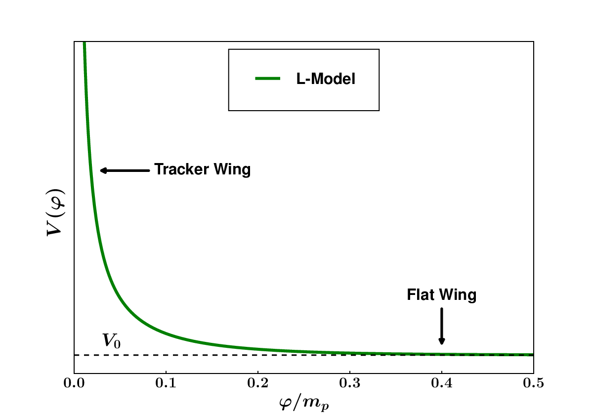
Consider first the L-model (9) and its natural extension³³ 3 We refer to this model as the ‘L-model’ since $V(\varphi)$ has a characteristic L shape for large values of $\lambda$ and $p$ as shown in figure 1.

For small values of the argument, $0<\frac{\lambda\varphi}{m_{p}}\ll 1$, one finds

which suggests that the early time behaviour of this model is very similar to that of the IPL model for which, at early times [4, 7]

where $w_{\rm B}$ is the background equation of state of matter/radiation. The IPL model (17) therefore has the appealing property that, for large values of $p\gg 1$, its EOS can track the EOS of the dominant matter component in the universe. Unfortunately it is also well known that, for $\Omega_{0m}\geq 0.2$, the IPL model (17) with $p>1$ cannot give rise to $w_{0}<-0.8$ at the present epoch [8]. This may be viewed as a significant shortfall of this model since observations appear to suggest that the current EOS of dark energy should satisfy $w_{0}\leq-0.9$ [13, 14, 15, 16, 17]. Of course this problem can be bypassed if one assumes a smaller value $p<1$ for the exponent in (17). However in this case the initial basin of attraction shrinks considerably, which diminishes the appeal of the IPL model.

The behavior of the L-potential (16) is illustrated in Fig. 2. The evolution of the scalar field energy density has been determined by solving the following system of equations relating to a spatially flat Friedman Robertson Walker (FRW) universe

where $\rho_{m}$ ($\rho_{r}$) is the density of matter (radiation), and the density and pressure of the scalar field are

As expected, the early time tracking phase in our model (16) – illustrated by figure 3, is identical to the tracking phase of the corresponding IPL potential $V\propto 1/\varphi^{p}$.

Figure 3 shows the evolution of $w_{\varphi}(z)=p_{\varphi}/\rho_{\varphi}$, in the L-potential $V=V_{0}\coth^{p}{\varphi/m_{p}}$ and in the IPL potential $V=V_{0}\left(\frac{m_{p}}{\varphi}\right)^{p}$. Note that both potentials have precisely two free parameters: $V_{0}$ and $p$. Fig. 3 draws attention to the interesting fact that, for the L-model with $V\sim\coth^{6}{\varphi}$, the current value of $w_{\varphi}$ can be as low as $w_{\varphi}\sim-0.8$, which is considerably lower than the corresponding value $w_{\varphi}\sim-0.4$ for $V\sim\varphi^{-6}$. In other words, for identical values of $p$, the late-time value of $w_{\varphi}$ in the L-model (16) is significantly lower than that in the IPL model (17). The value of $w_{\varphi}$ can be further lowered by increasing the value of $\lambda$ in (16), as shown in figure 3. The black star on the right y-axis of figure 3 indicates the observational $2\sigma$ upper bound, $w_{0}\leq-0.9$, for DE models with a slowly varying EOS⁵⁵ 5 The current $2\sigma$ upper bound on the EOS varies between $-0.8$ to $-0.9$, depending upon the data sets employed and the method of reconstruction [17]. We assume the conservative bound $w_{0}\leq-0.9$ to highlight the fact that the EOS in our models can drop to sufficiently low values at late times. [17].

Figure 4 shows the phase-space trajectories of the equation of state $\{w_{\varphi},w_{\varphi}^{\prime}\}$ starting from the matter dominated epoch. Here [27, 28]

Note that all trajectories approach the $\Lambda$CDM  limit ($w_{\varphi}=-1,w_{\varphi}^{\prime}=0$) at late times. The present epoch is marked by a circle on each trajectory. Comparing the L-model (16) with the IPL potential (17) we find that the current EOS in the former is always more negative than that in the latter, ie  $w_{0}^{\rm L1}<w_{0}^{\rm IPL}$, which supports our earlier results in fig. 3. Setting $\lambda=1$ in (16) and increasing the value of $p$ leads to $w_{\varphi}^{\prime}$ decreasing while $w_{\varphi}$ increases. On the other hand, increasing $\lambda$ (with $p$ held fixed) leads to the opposite behaviour, namely $w_{\varphi}$ decreases whereas $w_{\varphi}^{\prime}$ increases. Note that for moderately large values of $\lambda$ and $p$ ($\lambda,p\sim{\rm few}$) the L-model (16) will have a large initial basin of attraction before converging to $w_{\varphi}\sim-1,w_{\varphi}^{\prime}\sim 0$ by the present epoch.

Next we turn our attention to the oscillatory tracker model (10), namely

For large values $\frac{\lambda|\varphi|}{m_{p}}\gg 1$, this potential has the asymptotic form

The exponential potential has been extensively studied in [4, 6, 11, 29]. In the context of a spatially flat FRW universe it is well known that for $\lambda^{2}>3(1+w_{\rm B})$ the late time attractor in this model has the same equation of state as the background fluid, namely $w_{\varphi}=w_{\rm B}$. The associated fractional density of the scalar field is

with nucleosynthesis constraints imposing the lower bound $\lambda\lower 3.87495pt\hbox{ $\mathrel{\mathop{\kern 0.0pt\sim}\limits^{>}}$}~5$ [6, 30], while the CMB constraints impose an even stronger lower bound $\lambda\geq 13$ [31, 32, 33].

For small values, $\frac{\lambda|\varphi|}{m_{p}}\ll 1$, the potential (24) has the limiting form

We see that, as in the case of (16), the late time asymptote for $V(\varphi)$ is once again the cosmological constant $V_{0}$. However the presence of $\varphi^{2}$ in (27) suggests that the late time approach of $w_{\varphi}$ to $-1$ will be oscillatory. This has been illustrated in figures 5, 6 and 7 which show $w_{\varphi}(z)$ and $\{w_{\varphi},w_{\varphi}^{\prime}\}$ for different values of $\lambda$.

From figure 5, it is clear that $w_{\varphi}=1/3,~0$ during the radiation and matter domination epochs respectively. However, at late times the scalar field begins to oscillate around the minimum of its potential (27). Since these oscillations are of decreasing amplitude, $w_{\varphi}$ asymptotically approaches $w_{\varphi}=-1$ at late times. Interestingly, for moderate values $5\leq\lambda\leq 10$, the present value of $w_{\varphi}$ can lie anywhere between $-1$ to $-0.9$, its precise value being determined by the phase of the oscillation. However for larger values $\lambda>10$, the scalar field completes several oscillations prior to the present epoch. Since the mean value of $\varphi(t)$ in (27) falls off as $\langle\varphi^{2}(t)\rangle^{1/2}\propto a^{-3/2}(t)$ it follows that in such models $w_{\varphi}\simeq-1$ today. This has been illustrated in fig. 5 and especially in fig. 6.

The following expression describes the EOS of dark energy during the oscillatory epoch

where $\varphi_{m}(t)$ is the peak oscillation amplitude whose value steadily decreases with time. Eq. (28) can be rewritten as

where the steady decline of $\dot{\varphi}^{2}(t)$ with time ensures that $w_{\varphi}\to-1$ at late times.

The previous analysis is substantiated by figure 7 which shows the evolution of the phase-space $\{w_{\varphi},w_{\varphi}^{\prime}\}$ for $\lambda=20,~30$ with filled black circles marking the present epoch ($\Omega_{0m}=0.3$). The substantial difference in $w_{\varphi}(z)$ for $5\leq\lambda\leq 30$ and $0\leq z\leq 3$ (see fig. 6), may allow such models to be differentiated from one another on the basis of the high quality data expected from dark energy surveys such as DES, Euclid and SKA.

Due to the presence of the exponential tracker asymptote (25), the oscillatory tracker model (24) has a very large initial basin of attraction, trajectories from which get funneled into the late time attractor $w_{\varphi}\simeq-1$. Our results, summarized in figure 8, demonstrate that initial density values covering a range of more than $40$ orders of magnitude at $z=10^{12}$, converge onto the attractor scaling solution represented by the solid red curve. This range substantially increases if we set our initial conditions at earlier times. For instance, upon setting $\{\varphi_{i},\dot{\varphi}_{i}\}$ at the GUT scale of $10^{14}\,{\rm GeV}$ ($z\sim 10^{26}$), the range of initial density values that converges to $\Omega_{0,{\rm DE}}\simeq 0.7$ spans an impressive $100$ orders of magnitude ! The oscillatory tracker potential therefore exhibits a very large degree of freedom in the choice of initial conditions. In particular it permits the possibility of equipartition, according to which the density of dark energy and radiation may have been comparable at very early times just after reheating. In our view this is a very compelling property of this DE model.⁶⁶ 6 See [34, 35] for a dynamical analysis of models based on similar potentials.

In passing it may be appropriate to point out that the CPL ansatz [36, 37]

which is frequently used to reconstruct the properties of DE from observations, may be unable to accommodate the oscillatory behaviour of $w_{\varphi}$ which characterizes this model. Non-parametric reconstruction is likely to work better for this class of potentials [2, 38, 39, 40].

The recliner potential⁷⁷ 7 The Recliner potential (32) presents a limiting case of the family of potentials studied in [11], also see [33].

possesses the asymptotic form $V\simeq V_{0}\exp{(-\frac{\lambda\varphi}{m_{p}})}$ for $\lambda|\varphi|\gg m_{p}$ ($\varphi<0$). This endows it with a large initial basin of attraction, due to which scalar field trajectories rolling down (32) approach a common evolutionary path from a wide range of initial conditions.

In the large $\varphi$ limit, $\lambda\varphi\gg m_{p}$, $V(\varphi)$ monotonically declines to $V(\varphi)\simeq V_{0}$. Therefore one expects the value of $w_{\varphi}$ to approach $w_{\varphi}\to-1$ at late times, without any intermediate oscillations. This behaviour is substantiated by figure 9. The fact that the current value of $w_{\varphi}$ can fall below $-0.9$ makes this model quite appealing since it can describe cosmic acceleration without the fine tuning of initial conditions. The evolution of $w_{\varphi}(z)$ near the present epoch is shown in figure 10. One finds that different values of $\lambda$ in (32) can clearly be distinguished on the basis of low redshift measurements of $w_{\varphi}(z)$. Consequently upcoming dark energy survey’s (DES, Euclid, SKA, etc.) may provide a unique opportunity to set bounds (or even determine) the value of $\lambda$ in (32).

Phase-space trajectories $\{w_{\varphi},w_{\varphi}^{\prime}\}$ for the Recliner potential (32) are illustrated in figure 11. Note that larger values of $\lambda$ in (32) result in smaller values of $w_{\varphi}$ and larger values of $w_{\varphi}^{\prime}$ at late times.

It is interesting that the Oscillating tracker potential (24) and the Recliner potential(32) have two free parameters each, $V_{0}$ and $\lambda$, precisely the same number as in the IPL model $V=V_{0}\varphi^{-p}$ and the tracker $V=V_{0}\exp{\left(-\frac{\lambda\varphi}{m_{p}}\right)}$.

The Margarita potential describes a model of transient dark energy

This potential has tracker-like wings and a flat intermediate region (see figure 12). It exhibits three asymptotic branches:

where $m_{1}^{2}=\frac{2V_{0}\lambda_{1}^{2}}{m_{p}^{2}}$ and $m_{2}^{2}=\frac{V_{0}\lambda_{2}^{2}}{m_{p}^{2}}$ with $m_{1}\gg m_{2}$.

As illustrated by the red curve in figure 13, the acceleration of the universe in this model is a transient phenomenon. It ends once the scalar field rolls to the minimum of $V(\varphi)$. From that point on the scalar field begins to oscillate and behave like dark matter. Consequently the universe reverts to matter dominated expansion after the current accelerating epoch is over, with an extra contribution to dark matter coming from the coherently oscillating scalar field.

As suggested by (34) – (36), the motion of the scalar field proceeds along three distinct stages each of which is reflected in the cosmic expansion history.

(i) Initially $\varphi(t)$ rolls down the exponential potential (34). During this phase the scalar field density scales like the background fluid (radiation/matter) driving the expansion of the universe. (ii) After the tracking phase is over, the scalar field oscillates around the flat wing of the potential shown in figure 12. During this phase the universe begins to accelerate, as demonstrated in figure 14. (iii) Finally, at late times, the scalar field gets trapped within the sharp oscillatory region of the potential (36); see figure 12. Oscillations of the scalar field during this stage make it behave like pressureless matter with $\left\langle w_{\varphi}\right\rangle=0$; see the red line in figures 13 and 16.

We therefore find that cosmic acceleration is sandwiched between two matter dominated epochs. The duration of the accelerating phase depends upon the gap between $\lambda_{1}$ and $\lambda_{2}$. Nucleosynthesis constraints limit $\lambda_{2}\geq 5$ whereas the only constraint on $\lambda_{1}$ comes from the inequality $\lambda_{1}\gg\lambda_{2}$.

At this point we would like to draw attention to a key feature of the Margarita potential which distinguishes this model of transient acceleration from others of its kind. Note that the asymptotic form of the potential within the flat wing, described by (35), bears close resemblance to the potential near $\varphi\simeq 0$ for the oscillatory tracker model, namely (27). Therefore, as in that model, one might expect $w_{\varphi}$ to approach $-1$ at late times via small oscillations. This would indeed be the case were it not for the presence of the sharp oscillatory region near $\varphi\simeq 0$ in fig. 12. This region modifies the behaviour of $\varphi$ significantly. As $\varphi$ traverses $\varphi\simeq 0$, its EOS abruptly changes from negative to positive values. This leads to a spike in the value of $w_{\varphi}$ and in the deceleration parameter $q$. An accelerating universe punctuated by periods of sudden deceleration therefore becomes a key feature of the Margarita model of DE, as shown in figures 14 & 15.

It is well known that, unlike $\Lambda$CDM, a transiently accelerating universe does not possess a future event horizon. Moreover the presence of even a tiny curvature term, $k/a^{2}$, can cause such a universe to stop expanding and begin to contract, giving rise to a very different cosmological future from $\Lambda$CDM. Note that while models of transient DE have been discussed earlier, see for instance [41, 42, 43], to the best of our knowledge none of these early models had a tracker-like commencement.

Finally the reader may be interesting in a companion potential to (33) which provides another example of transient dark energy with tracker-like behaviour at early times

References

- (1) V. Sahni and A.A. Starobinsky, Int. J. Mod. Phys. D9 373 (2000).
- (2) V. Sahni and A.A. Starobinsky, Int. J. Mod. Phys. D15 2105 (2006).
- (3) P. J. E. Peebles and B. Ratra, Rev. Mod. Phys. 75 559 (2003); T. Padmanabhan, Phys. Rep. 380 235 (2003); V. Sahni, [astro-ph/0202076], [astro-ph/0502032]; V. Sahni, Dark matter and dark energy, Lect. Notes Phys. 653, 141-180 (2004) [astro-ph/0403324]. E. J. Copeland, M. Sami and S. Tsujikawa, Int. J. Mod. Phys. D15 1753 (2006); R. Bousso, Gen. Relativ. Gravit. 40, 607 (2008); L. Amendola and S. Tsujikawa, Dark Energy, Cambridge University Press, 2010.
- (4) B. Ratra and P.J.E. Peebles, Phys. Rev. D 37, 3406 (1988).
- (5) C. Wetterich, Nuclear Physics B 302, 668 (1988).
- (6) P.G. Ferreira and M. Joyce, Phys. Rev. Lett. 79, 4740 (1997); P.G. Ferreira, P.G. and M. Joyce, Phys. Rev. D 58, 023503 (1998).
- (7) I. Zlatev L. Wang and P.J. Steinhardt, Phys. Rev. Lett. 82, 896 (1999).
- (8) P.J. Steinhardt, L. Wang and I. Zlatev, Phys. Rev. D 59, 123504 (1999).
- (9) V. Sahni and L. Wang, Phys. Rev. D 62, 103517 (2000).
- (10) P. Brax and J. Martin, Phys. Rev. D 61, 103502 (2000); Phys. Lett. B 468, 40 (1999).
- (11) T. Barreiro, E.J. Copeland and N.J. Nunes, Phys. Rev. D 61, 127301 (2000).
- (12) A. Albrecht and C. Skordis, Phys. Rev. Lett. 84, 2076 (2000).
- (13) Y. Wang et al., SDSS Collaboration, MNRAS 469, 3762 (2017) [arXiv:1607.03154].
- (14) S. Alam et al., BOSS Collaboration, MNRAS 470, 2617 (2017) [arXiv:1607.03155].
- (15) P.A.R. Ade et al., Planck Collaboration, Astron. Astrophys. 594, A14 (2016), Dark energy and modified gravity, [arXiv:1502.01590].
- (16) A. I. Lonappan, Ruchika, A. A Sen, arXiv:1705.07336.
- (17) D. Huterer and D.L. Shafer, Rep. Prog. Phys. 81, 016901 (2018) [arXiv:1709.01091].
- (18) R. Kallosh and A. Linde, JCAP07 (2013) 002 [arXiv:1306.5220].
- (19) R. Kallosh, A. Linde and D. Roest, JHEP11, 198 (2013) [arXiv:1311.0472].
- (20) S. Mishra, V. Sahni and Yu. Shtanov, JCAP 06(2017)045 [arXiv:1703.03295]
- (21) E. V. Linder, Phys. Rev. D 91, no. 12, 123012 (2015) [arXiv:1505.00815].
- (22) A. Kamenshchik, U. Moschella and V. Pasquier, 2001, Phys. Lett. B 511, 265 [gr-qc/0103004].
- (23) V. Gorini, A. Kamenshchik, U. Moschella, V. Pasquier and A. Starobinsky, 2005, Phys. Rev. D 72, 103518 [astro-ph/0504576].
- (24) N. Bilic, G.B. Tupper and R. Viollier, 2002, Phys. Lett. B 535, 17 [astro-ph/0111325].
- (25) A. Frolov, L. Kofman and A. Starobinsky, 2002, Phys. Lett. B 545, 8 [hep-th/0204187].
- (26) S. Matarrese, C. Baccigalupi and F. Perrotta, Phys. Rev. D 70, 061301 (2004).
- (27) R.R. Caldwell and E.V. Linder, Phys. Rev. Lett. 95, 141301 (2005).
- (28) E.V. Linder, Astropart. Phys. 91, 11 (2017) [arXiv:1701.01445].
- (29) V. Sahni, H. Feldman and A. Stebbins, Astrophys.J. 385, 1, (1992).
- (30) E.J. Copeland, A.R. Liddle and D. Wands, Phys. Rev. D 57, 4686 (1998).
- (31) E. Calabrese, D. Huterer, E. V. Linder, A. Melchiorri and L. Pagano, Phys. Rev. D 83, 123504 (2011) [arXiv:1103.4132 [astro-ph.CO]].
- (32) A. Hojjati, E. V. Linder and J. Samsing, Phys. Rev. Lett. 111, 041301 (2013) [arXiv:1304.3724 [astro-ph.CO]].
- (33) H. Chang, R. J. Scherrer, [arXiv:1608.03291].
- (34) N. Roy and N. Banerjee, Gen. Rel. Grav. 46, 1651 (2014) [arXiv:1312.2670 [gr-qc]].
- (35) A. Paliathanasis, M. Tsamparlis, S. Basilakos and J. D. Barrow, Phys. Rev. D 91, no. 12, 123535 (2015) [arXiv:1503.05750 [gr-qc]].
- (36) M. Chevallier and D. Polarski, Int. J. Mod. Phys. D 10, 213 (2001) [gr-qc/0009008].
- (37) E. V. Linder, Phys. Rev. Lett. 90, 091301 (2003) [astro-ph/0208512].
- (38) A. Shafieloo, U. Alam, V. Sahni, and A.A. Starobinsky, Mon. Not. R. Astron. Soc. 366, 1081 (2006); J. Dick,L. Knox, and M. Chu, J. Cosmol. Astropart. Phys. 07 (2006) 001; A. Shafieloo, Mon. Not. R. Astron. Soc. 380, 1573 (2007); D. Huterer and G. Starkman, Phys. Rev. Lett. 90, 031301 (2003); R. G. Crittenden, L. Pogosian, and G. B. Zhao, J. Cosmol. Astropart. Phys. 12 (2009) 025; C. Clarkson and C. Zunckel, Phys. Rev. Lett. 104, 211301 (2010); R. G. Crittenden, G. B. Zhao, L. Pogosian, L. Samushia, and X. Zhang, J. Cosmol. Astropart. Phys. 02 (2012) 048; T. Holsclaw, U. Alam, B. Sanso´, H. Lee, K. Heitmann, S. Habib, and D. Higdon, Phys. Rev. Lett. 105, 241302 (2010); A. Shafieloo, A. G. Kim, and E.V. Linder, Phys. Rev. D 85, 123530 (2012); M. Seikel, C. Clarkson, and M. Smith, J. Cosmol. Astropart. Phys. 06 (2012) 036.
- (39) G-B. Zhao, R. G. Crittenden, L. Pogosian and X. Zhang, Phys. Rev. Lett. 109, 171301 (2012).
- (40) G-B Zhao, et. al., Nature Astronomy 1, 627 (2017).
- (41) J. Frieman, C.T. Hill, A. Stebbins and I. Waga, Phys. Rev. Lett. 75, 2077 (1995); K. Choi, Phys.Rev. D 62 043509 (2000) [hep-ph/9902292]; J.D. Barrow, R. Bean, and J. Magueijo, MNRAS 316, L41 (2000); S.C. Ng and D.L. Wiltshire, Phys.Rev. D 64 123519 (2001) [astro-ph/0107142]; R. Kallosh, A. Linde, S. Prokushkin and M. Shmakova, Phys. Rev. D 66 123503 (2002) [arXiv:hep-th/0208156]; R. Kallosh and A. Linde, JCAP 02 02 (2003) [astro-ph/0301087]; U. Alam, V. Sahni and A.A. Starobinsky, JCAP 0304, 002 (2003) [astro-ph/0302302].
- (42) V. Sahni and Yu.V. Shtanov JCAP 0311,014, (2003) astro-ph/0202346.
- (43) A. Shafieloo, D.K. Hazra, V. Sahni and A. A. Starobinsky, Metastable Dark Energy with Radioactive-like Decay, arXiv:1610.05192.
- (44) V. Sahni and A. A. Sen, Eur.Phys.J. C77, 225 (2017) [arXiv:1510.09010]