跳到论文正文
W Papers独立论文阅读器 arXiv:1709.08970 论文正文 计算阅读时间 · 0%
引用这篇论文根据当前论文元数据生成,正式投稿前建议核对。


License: arXiv.org perpetual non-exclusive license
arXiv:1709.08970v1 [hep-ph] 26 Sep 2017

Back-to-back heavy quark pair production in Semi-inclusive DIS

Guang-Peng Zhang Affiliation: Department of modern physics, University of Science and Technology of China, Hefei, Anhui 230026, China
Abstract

The one-loop correction to heavy quark pair back-to-back production in unpolarized semi-inclusive deep inelastic scattering is given in this work in the framework of transverse momentum dependent(TMD) factorization. Both unpolarized and linearly polarized TMD gluon distribution functions are taken into account. A subtraction method based on diagram expansion is used to get finite hard coefficients. It is found the soft and collinear divergences of one-loop amplitude is proportional to tree level ones and can be expressed through several basic scalar triangle and bubble integrals. The subtraction of these divergences is spin independent. Beyond tree level an additional soft factor related to final heavy quark pair must be added into the factorization formula. This soft factor affects the azimuthal angle distribution of virtual photon in a nonperturbative way. Integrating over virtual photon azimuthal angle we construct three weighted cross sections, which depend on only three additional integrated soft factors. These weighted cross sections can be used to extract linearly polarized gluon distribution function. In addition, lepton azimuthal angle is unintegrated in this work, which provides more observables. All hard coefficients relevant to lepton and virtual photon azimuthal angle distributions are given at one-loop level.

I Introduction

Gluon transverse momentum dependent(TMD) distribution functions take important information about the hadron structure. In high energy region, gluon as a parton usually plays more important role than quark, since the momentum fraction of parton is always very small. Thus, precise knowledge of gluon distribution functions is desired to make precise prediction of the cross section. Since gluon is spin-1, it can have different polarizations in a hadron. When the transverse momentum of the gluon in a hadron is integrated over, there is only one gluon distribution function possible for unpolarized hadron, which is the usual collinear gluon parton distribution function(PDF). In such integrated PDF the gluon is unpolarized. But when the transverse momentum of gluon is unintegrated, the transverse momentum of gluon can couple with the spin of gluon to give a description of polarized distribution of gluon in a hadron[1]. For unpolarized hadron, there exists two such transverse momentum dependent gluon distribution functions: one is denoted as G⁡(x,p⟂2)G(x,p_{\perp}^{2}), which reflects the distribution of unpolarized gluon in a hadron, with longitudinal momentum fraction xx and transverse momentum p⟂p_{\perp}, the other is H⟂​(x,p⟂2)H^{\perp}(x,p_{\perp}^{2}), which reflects the distribution of linearly polarized gluon in the hadron. So far, the second gluon distribution function, i.e., H⟂​(x,p⟂2)H^{\perp}(x,p_{\perp}^{2}) has already aroused much interest in current researches, such as the effect of H⟂H^{\perp} on higgs boson production at LHC[2, 3, 4, 5, 6]. One can see e.g.,[7, 8] for a review on linearly polarized gluon distribution function. Various schemes are proposed to extract this function in literature. For hadron reaction, pair photon production[9], photon-quarkonium[10] or quarkonium-quarkonium[11] associated production are proposed to extract this function from a cos⁡(2​ϕ)\cos(2\phi) azimuthal angle distribution in these reactions. For hadron reaction, the problem is the potential breaking of TMD factorization as pointed out in [12],[13]. All these proposed schemes require the detected final states are colorless(for quarkonium the heavy quark pair from hard interaction is in a color singlet). Contrast to hadron reaction, semi-inclusive deep inelastic scattering(SIDIS) for heavy quark pair or di-jet production is expect to have an exact TMD factorization, and can be used to extract some definite information about gluon TMD distribution functions. [14] have examined the effect of H⟂H^{\perp} in heavy quark pair and di-jet production. For heavy quark pair production, the study in [14] is at tree level or leading order of αs\alpha_{s} with a simplified TMD formula. At this order the TMD formula just contains gluon TMD distribution functions as nonperturbative quantities. To higher order of αs\alpha_{s}, the soft radiation from final heavy quark pair will introduce an azimuthal angle dependent soft factor into TMD formula and affect the azimuthal angle distribution of virtual photon,i.e., ϕq\phi_{q}, which is used to extract H⟂H^{\perp} in [14]. Because of the azimuthal angle dependent soft factor, a complete description of ϕq\phi_{q} distribution in the cross section is impossible. Instead we construct three azimuthal angle weighted cross sections, which depend on only three integrated soft factors. These weighted cross sections may help to extract H⟂H^{\perp}. In [15], the TMD factorization for this process is examined at one-loop level, with H⟂H^{\perp} not taken into account. It is found all collinear and soft divergences can be absorbed into gluon distribution function and a soft factor with azimuthal angle integrated. But part of the finite correction of hard coefficients is absent in [15], and the study is confined to G⁡(x,p⟂2)G(x,p_{\perp}^{2}). In this paper, we want to study the azimuthal angle effect introduced by the soft factor mentioned above. We will examine the factorization formula for both G⁡(x,p⟂)G(x,p_{\perp}) and H⟂​(x,p⟂)H^{\perp}(x,p_{\perp}) based on diagram expansion method presented in [16]. This method is different from the method in [15], which uses a single gluon to replace initial hadron. The method based on diagram expansion enables us to obtain the finite hard coefficients for various parton distributions in a systematic way. In addition, we keep lepton azimuthal angle unintegrated in this work, which can provide more observables. The structure of this paper is as follows: in Sect.II we illustrate kinematics for heavy quark pair production in SIDIS; in Sect.III, tree level factorization and resulting angular distributions are discussed, including lepton azimuthal angle distributions; in Sect.IV, the factorization formula is examined at one-loop level and the hard coefficients are calculated. In this section, the soft factors are also constructed and virtual one-loop corrections to soft factors and distribution functions are calculated; in Sect.V, the effect of soft factor is discussed and three weighted cross sections are constructed to extract H⟂H^{\perp}; Sect.VI is our summary.

II Kinematics

We consider the scattering of electron and hadron

e⁡(l)+hA​(PA)→e⁡(l′)+Q⁡(k1)+Q¯​(k2)+X,\displaystyle e(l)+h_{A}(P_{A})\rightarrow e(l^{\prime})+Q(k_{1})+\bar{Q}(k_{2})+X, (1)

where XX represents undetected hadrons[17]. At order of αe​m2\alpha_{em}^{2}, this process is dominated by the exchange of a virtual photon between electron and hadron. The momentum of the virtual photon is qμ=lμ−l′μq^{\mu}=l^{\mu}-{l^{\prime}}^{\mu}. In perturbative region, Q2=−q2≫ΛQ​C​D2Q^{2}=-q^{2}\gg\Lambda_{QCD}^{2}. Q,Q¯Q,\bar{Q} with momenta k1,k2k_{1},k_{2} are heavy quark and anti-quark produced in the hard collision. In the center of mass(c.m.) frame of virtual photon γ∗\gamma^{*} and initial hadron hAh_{A}, we demand QQ and Q¯\bar{Q} are nearly back-to-back.

For convenience we define

Kμ=k1μ+k2μ,Rμ=12​(k1μ−k2μ).\displaystyle K^{\mu}=k_{1}^{\mu}+k_{2}^{\mu},\ R^{\mu}=\frac{1}{2}(k_{1}^{\mu}-k_{2}^{\mu}). (2)

Our requirement for the final quarks then becomes

RTμ∼Q,KTμ≪Q,\displaystyle R_{T}^{\mu}\sim Q,\ K_{T}^{\mu}\ll Q, (3)

where RTR_{T} and KTK_{T} are the transverse components of RR and KK, respectively. In the c.m. frame of γ∗\gamma^{*} and hAh_{A}, the transverse vector is relative to ZZ-axis. Here P→A\vec{P}_{A} is along +Z+Z-axis, and q→\vec{q} is along −Z-Z-axis.

By considering only the contribution of virtual photon, the cross section we want to study can be written as

d​σ=12​s​e4​Qq2Q4​(2​π)4​d3​l′(2​π)3​2​l′0​d3​k1(2​π)3​2​E1​d3​k2(2​π)3​2​E2​Lμ​ν​Wμ​ν,\displaystyle d\sigma=\frac{1}{2s}\frac{e^{4}Q_{q}^{2}}{Q^{4}}(2\pi)^{4}\frac{d^{3}l^{\prime}}{(2\pi)^{3}2{l^{\prime}}^{0}}\frac{d^{3}k_{1}}{(2\pi)^{3}2E_{1}}\frac{d^{3}k_{2}}{(2\pi)^{3}2E_{2}}L^{\mu\nu}W_{\mu\nu}, (4)

where the leptonic and hadronic tensors are

Lμ​ν=\displaystyle L^{\mu\nu}= 2​(lμ​l′ν+lν​l′μ−gμ​ν​l⋅l′)≐4​lμ​lν+q2​gμ​ν;\displaystyle 2(l^{\mu}{l^{\prime}}^{\nu}+l^{\nu}{l^{\prime}}^{\mu}-g^{\mu\nu}l\cdot l^{\prime})\doteq 4l^{\mu}l^{\nu}+q^{2}g^{\mu\nu};
Wμ​ν=\displaystyle W^{\mu\nu}= ∑X⟨PA​s|jν​|Q​Q¯​X⟩​⟨Q​Q¯​X|​jμ​(0)|PA​s⟩​δ4​(PA+q−k1−k2−PX).\displaystyle\sum_{X}\langle P_{A}s|j^{\nu}|Q\bar{Q}X\rangle\langle Q\bar{Q}X|j^{\mu}(0)|P_{A}s\rangle\delta^{4}(P_{A}+q-k_{1}-k_{2}-P_{X}). (5)

In leptonic tensor we have used QED gauge invariance qμ​Wμ​ν=0q^{\mu}W_{\mu\nu}=0 to eliminate all qμq^{\mu} and qνq^{\nu} in leptonic tensor. This will simplify our calculation.

Define

xB=Q22​PA⋅q,y=PA⋅qPA⋅l,z1=PA⋅k1PA⋅q,z2=PA⋅k2PA⋅q,s=(PA+l)2.\displaystyle x_{B}=\frac{Q^{2}}{2P_{A}\cdot q},\hskip 14.22636pty=\frac{P_{A}\cdot q}{P_{A}\cdot l},\hskip 14.22636ptz_{1}=\frac{P_{A}\cdot k_{1}}{P_{A}\cdot q},\hskip 14.22636ptz_{2}=\frac{P_{A}\cdot k_{2}}{P_{A}\cdot q},\hskip 14.22636pts=(P_{A}+l)^{2}. (6)

The phase space integration measure can be written as

d3​l′2​l′0=y​s4​d​xB​d​y​d​ψl,d3​k12​E1​d3​k22​E2=14​d​y1​d​y2​d2​KT​d2​RT,\displaystyle\frac{d^{3}l^{\prime}}{2{l^{\prime}}^{0}}=\frac{ys}{4}dx_{B}dyd\psi_{l},\hskip 28.45274pt\frac{d^{3}k_{1}}{2E_{1}}\frac{d^{3}k_{2}}{2E_{2}}=\frac{1}{4}dy_{1}dy_{2}d^{2}K_{T}d^{2}R_{T}, (7)

where ψl\psi_{l} is the azimuthal angle between l′T{l^{\prime}}_{T} and RTR_{T}; y1,2y_{1,2} are the rapidities of final quark and anti-quark, respectively.

Then, the differential cross section becomes

d​σd​xB​d​y​d​ψl​d​y1​d​y2​d2​KT​d2​RT=y​αe​m2​Qq264​π3​Q4​Lμ​ν​Wμ​ν,\displaystyle\frac{d\sigma}{dx_{B}dyd\psi_{l}dy_{1}dy_{2}d^{2}K_{T}d^{2}R_{T}}=\frac{y\alpha_{em}^{2}Q_{q}^{2}}{64\pi^{3}Q^{4}}L^{\mu\nu}W_{\mu\nu}, (8)

where QqQ_{q} is the electric charge of heavy quark in unit of the charge of electron. All information about the cross section now is contained in the hadronic tensor Wμ​νW^{\mu\nu}. In next sections we will focus on the factorization of hadronic tensor.

γ∗​N\gamma^{*}N frame(c.m. frame of γ∗\gamma^{*} and hAh_{A}) is useful to describe the cross section, but it is not very convenient for the calculation, especially for the factorization of Wμ​νW^{\mu\nu}, as we discussed later. More convenient frame is the hadron frame defined as the c.m. frame of final heavy quark and antiquark. In this frame, P→A\vec{P}_{A} is still along +Z+Z-axis, but virtual photon now has a small transverse momentum q⟂q_{\perp}. We use light-cone coordinate representation in this paper. In this representation any vector aμa^{\mu} is written as (a+,a−,a⟂μ)(a^{+},a^{-},a_{\perp}^{\mu}), where the transverse components are relative to ZZ-axis and denoted by a⟂a_{\perp}; ±\pm-components are defined by two light-like vectors nμn^{\mu} and n¯μ\bar{n}^{\mu} with n⋅n¯=1n\cdot\bar{n}=1, i.e., a+=n⋅aa^{+}=n\cdot a, a−=n¯⋅aa^{-}=\bar{n}\cdot a. The decomposition of relevant momenta is like

PAμ=PA+​n¯μ,Kμ=K+​n¯μ+K−​nμ,qμ=q+​n¯μ+q−​nμ+q⟂μ.\displaystyle P_{A}^{\mu}=P_{A}^{+}\bar{n}^{\mu},\ K^{\mu}=K^{+}\bar{n}^{\mu}+K^{-}n^{\mu},\ q^{\mu}=q^{+}\bar{n}^{\mu}+q^{-}n^{\mu}+q_{\perp}^{\mu}. (9)

The following two tensors are useful to project transverse components of a vector:

g⟂μ​ν=gμ​ν−nμ​n¯ν−nν​n¯μ,ϵ⟂μ​ν=ϵμ​ν−+=ϵμ​ν​ρ​τ​n¯ρ​nτ,\displaystyle g_{\perp}^{\mu\nu}=g^{\mu\nu}-n^{\mu}\bar{n}^{\nu}-n^{\nu}\bar{n}^{\mu},\ \ \epsilon_{\perp}^{\mu\nu}=\epsilon^{\mu\nu-+}=\epsilon^{\mu\nu\rho\tau}\bar{n}_{\rho}n_{\tau}, (10)

and our convention for ϵ\epsilon-tensor is ϵ0123=1\epsilon^{0123}=1 so that ϵ⟂12=1\epsilon_{\perp}^{12}=1. For any four-vector aμa^{\mu} its transverse component is a⟂μ=g⟂μ​ν​aνa_{\perp}^{\mu}=g_{\perp}^{\mu\nu}a_{\nu}.

Given these two frames, q⟂q_{\perp} in hadron frame and KTK_{T} in γ∗​N\gamma^{*}N frame can be connected to each other. In γ∗​N\gamma^{*}N frame,

KTμ=Kμ−α​PAμ−β​qμ.\displaystyle K_{T}^{\mu}=K^{\mu}-\alpha P_{A}^{\mu}-\beta q^{\mu}. (11)

Hence, the transverse component of KTK_{T} in the hadron frame is

(KT)⟂μ=−β​q⟂μ=−(z1+z2)​q⟂μ.\displaystyle(K_{T})_{\perp}^{\mu}=-\beta q_{\perp}^{\mu}=-(z_{1}+z_{2})q_{\perp}^{\mu}. (12)

On the other hand,

(KT)⟂μ=g⟂μ​ν​KT​ν=KTμ−PAμ​KT2PA⋅K.\displaystyle(K_{T})_{\perp}^{\mu}=g_{\perp}^{\mu\nu}K_{T\nu}=K_{T}^{\mu}-P_{A}^{\mu}\frac{K_{T}^{2}}{P_{A}\cdot K}. (13)

Combining these two equations we have

KTμ=−(z1+z2)​q⟂μ+PAμ​KT2PA⋅K.\displaystyle K_{T}^{\mu}=-(z_{1}+z_{2})q_{\perp}^{\mu}+P_{A}^{\mu}\frac{K_{T}^{2}}{P_{A}\cdot K}. (14)

This is an exact result. In the region we are considering, KTK_{T} is a small quantity, then the second term with KT2K_{T}^{2} can be ignored at leading power level.

In this work all calculations will be performed in hadron frame. To define azimuthal angles on the transverse plane we assign k→1⟂\vec{k}_{1\perp} along +X+X-axis, and YY-axis is defined by ϵ⟂\epsilon_{\perp}-tensor, that is,

Xμ=k1⟂μ|k→1⟂|,Yμ=ϵ⟂μ​ν​Xν.\displaystyle X^{\mu}=\frac{k_{1\perp}^{\mu}}{|\vec{k}_{1\perp}|},\ Y^{\mu}=\epsilon_{\perp}^{\mu\nu}X_{\nu}. (15)

Then the azimuthal angles of virtual photon and initial lepton, ϕq\phi_{q} and ϕl\phi_{l}, are defined as the angles of q⟂q_{\perp} and l⟂l_{\perp} relative to XX-axis, respectively, as shown in Fig.1. At leading power of q⟂q_{\perp} expansion, ϕl\phi_{l} is equal to ψl\psi_{l}, which is defined in γ∗​N\gamma^{*}N frame.

Refer to caption
Figure 1: Azimuthal angles of virtual photon and initial lepton in the transverse plane of hadron frame.

With these two vectors XμX^{\mu} and YμY^{\mu} the transverse metric and anti-symmetric tensor can be written into another form

g⟂μ​ν=−Xμ​Xν−Yμ​Yν,ϵ⟂μ​ν=Xμ​Yν−Xν​Yμ.\displaystyle g_{\perp}^{\mu\nu}=-X^{\mu}X^{\nu}-Y^{\mu}Y^{\nu},\ \epsilon_{\perp}^{\mu\nu}=X^{\mu}Y^{\nu}-X^{\nu}Y^{\mu}. (16)

Since n,n¯,X,Yn,\bar{n},X,Y form a complete basis in four-dimension space, the leptonic tensor can be expressed through these four vectors. Equivalently, one can choose PA,K,X,YP_{A},K,X,Y as basis. The advantage of this basis is the calculation can be done in a covariant way.

The complete basis for symmetric rank-2 tensor is

Aiμ​ν=\displaystyle A_{i}^{\mu\nu}= {n~μ​n~ν,n~μ​Xν+n~ν​Xμ,n~μ​Yν+n~ν​Yμ,Xμ​Xν+Yμ​Yν,Xμ​Xν−Yμ​Yν,Xμ​Yν+Xν​Yμ},i=1,⋯,6.\displaystyle\left\{\tilde{n}^{\mu}\tilde{n}^{\nu},\tilde{n}^{\mu}X^{\nu}+\tilde{n}^{\nu}X^{\mu},\ \tilde{n}^{\mu}Y^{\nu}+\tilde{n}^{\nu}Y^{\mu},\ X^{\mu}X^{\nu}+Y^{\mu}Y^{\nu},\ X^{\mu}X^{\nu}-Y^{\mu}Y^{\nu},\ X^{\mu}Y^{\nu}+X^{\nu}Y^{\mu}\right\},\hskip 14.22636pti=1,\cdots,6. (17)

With this basis leptonic tensor in hadron frame is expressed as

Lμ​ν=\displaystyle L^{\mu\nu}= Q2​4​(1−y)y2​n~μ​n~ν+Q2​1+(1−y)2y2​(Xμ​Xν+Yμ​Yν)\displaystyle Q^{2}\frac{4(1-y)}{y^{2}}\tilde{n}^{\mu}\tilde{n}^{\nu}+Q^{2}\frac{1+(1-y)^{2}}{y^{2}}(X^{\mu}X^{\nu}+Y^{\mu}Y^{\nu})
+2Q21−y​(y−2)y2cosϕl(n~μXν+n~νXμ)+2Q21−y​(y−2)y2sinϕl(n~μYν+n~νYμ)\displaystyle+2Q^{2}\frac{\sqrt{1-y}(y-2)}{y^{2}}\cos\phi_{l}(\tilde{n}^{\mu}X^{\nu}+\tilde{n}^{\nu}X^{\mu})+2Q^{2}\frac{\sqrt{1-y}(y-2)}{y^{2}}\sin\phi_{l}(\tilde{n}^{\mu}Y^{\nu}+\tilde{n}^{\nu}Y^{\mu})
+2​Q2​1−yy2​cos⁡(2​ϕl)​(Xμ​Xν−Yμ​Yν)+2​Q2​1−yy2​sin⁡(2​ϕl)​(Xμ​Yν+Xν​Yμ),\displaystyle+2Q^{2}\frac{1-y}{y^{2}}\cos(2\phi_{l})(X^{\mu}X^{\nu}-Y^{\mu}Y^{\nu})+2Q^{2}\frac{1-y}{y^{2}}\sin(2\phi_{l})(X^{\mu}Y^{\nu}+X^{\nu}Y^{\mu}), (18)

where

n~μ=12​αk​PA⋅K+αk2​K2​(PA+αk​K)μ,αk=−PA⋅qK⋅q.\displaystyle\tilde{n}^{\mu}=\frac{1}{\sqrt{2\alpha_{k}P_{A}\cdot K+\alpha_{k}^{2}K^{2}}}(P_{A}+\alpha_{k}K)^{\mu},\ \alpha_{k}=-\frac{P_{A}\cdot q}{K\cdot q}. (19)

In the decomposition we have considered the constraint of QED gauge invariance, that is, PAμP_{A}^{\mu} and KμK^{\mu} must be combined into n~μ\tilde{n}^{\mu} to ensure qμ​Aiμ​ν=0q_{\mu}A_{i}^{\mu\nu}=0. Since q⋅X∼q⋅Y∼𝒪⁡(q⟂)q\cdot X\sim q\cdot Y\sim\mathcal{O}(q_{\perp}), QED gauge invariance is preserved at leading power of q⟂q_{\perp}. One can check that n~μ\tilde{n}^{\mu} can have another representation like

n~μ=1Q​(q+2​xB​PA)μ+𝒪⁡(q⟂).\displaystyle\tilde{n}^{\mu}=\frac{1}{Q}(q+2x_{B}P_{A})^{\mu}+\mathcal{O}(q_{\perp}). (20)

This representation simplifies our calculation dramatically. Since hadronic tensor does not depend on ϕl\phi_{l}, this decomposition exhibits all possible lepton azimuthal angle distributions for unpolarized lepton beam.

III Tree level azimuthal angle dependence

In hadron frame when q⟂q_{\perp} is small, Wμ​νW^{\mu\nu} can have a TMD factorization formula at the leading power of q⟂q_{\perp} expansion. At tree level the formula reads

Wμ​ν=\displaystyle W^{\mu\nu}= xBx​Q2​Mp​(Nc2−1)​δ​(1−z1−z2)​Hα​βμ​ν​∫d2​p⟂​δ2​(p⟂+q⟂)​Φα​β​(x,p⟂)+𝒪⁡(q⟂Q,q⟂k1⟂),\displaystyle\frac{x_{B}}{xQ^{2}M_{p}(N_{c}^{2}-1)}\delta(1-z_{1}-z_{2})H^{\mu\nu}_{\alpha\beta}\int d^{2}p_{\perp}\delta^{2}(p_{\perp}+q_{\perp})\Phi^{\alpha\beta}(x,p_{\perp})+\mathcal{O}(\frac{q_{\perp}}{Q},\frac{q_{\perp}}{k_{1\perp}}), (21)

where the gluon TMDPDF is[1]

Φα​β​(x,p⟂)=\displaystyle\Phi^{\alpha\beta}(x,p_{\perp})= (p+2​Mp)−1​∫d​ξ−​d2​ξ⟂(2​π)3​ei​x​ξ−​PA++i​ξ⟂⋅p⟂​⟨PA|​Ga⟂+β​(0)​Ga⟂+α​(0+,ξ−,ξ⟂)​|PA⟩\displaystyle\left(\frac{p^{+}}{2M_{p}}\right)^{-1}\int\frac{d\xi^{-}d^{2}\xi_{\perp}}{(2\pi)^{3}}e^{ix\xi^{-}P_{A}^{+}+i\xi_{\perp}\cdot p_{\perp}}\langle P_{A}|G_{a\perp}^{+\beta}(0)G_{a\perp}^{+\alpha}(0^{+},\xi^{-},\xi_{\perp})|P_{A}\rangle
=\displaystyle= −g⟂α​β​G​(x,p⟂2)+2​p⟂α​p⟂β−g⟂α​β​p⟂22​Mp2​H⟂​(x,p⟂2),\displaystyle-g_{\perp}^{\alpha\beta}G(x,p_{\perp}^{2})+\frac{2p_{\perp}^{\alpha}p_{\perp}^{\beta}-g_{\perp}^{\alpha\beta}p_{\perp}^{2}}{2M_{p}^{2}}H^{\perp}(x,p_{\perp}^{2}), (22)

We work in Feynman gauge ∂μGμ=0\partial^{\mu}G_{\mu}=0 in this work. The gauge links in Φα​β\Phi^{\alpha\beta} are suppressed for simplicity. There is a color summation in the definition of gluon TMDPDF. Therefore, there is a color average in the hard part. In formula eq.(21), the average factor 1/(Nc2−1)1/(N_{c}^{2}-1) has been extracted, so, the hard part Hα​βμ​νH^{\mu\nu}_{\alpha\beta} in eq.(21) contains a summation over color.

The derivation of this factorization formula for hadronic tensor has been given in [18] in detail. Under high energy limit or Q2→∞Q^{2}\to\infty, the general structure of the interaction factorizes into the form shown in Fig.2, where the two central bubbles represent hard interaction, in which all propagators are far off-shell, and the lower bubble represents the jet part of initial hadron, in which all propagators are collinear to PAP_{A}. All possible soft interactions are ignored in Fig.2. These soft interactions do not appear at the leading order of αs\alpha_{s}. We will discuss them in one-loop correction.

Refer to caption
Figure 2: TMD factorization for heavy quark pair production in DIS. The two central bubbles represent hard subprocess, while lower bubble represents jet part of initial hadron.

For this process, the hard scales are QQ and k1⟂k_{1\perp}, which are taken to be the same order in this paper. Under the limit q⟂≪Q,k1⟂q_{\perp}\ll Q,k_{1\perp}, the above factorization formula is obtained from the expansion in λ≃q⟂/Q,q⟂/k1⟂\lambda\simeq q_{\perp}/Q,\ q_{\perp}/k_{1\perp}. Leading power contribution of this process is given by collinear partons, that is, the momentum of initial gluon satisfies pμ=(p+,p−,p⟂)∼Q⁡(1,λ2,λ)p^{\mu}=(p^{+},p^{-},p_{\perp})\sim Q(1,\lambda^{2},\lambda). According to this scaling law p⟂p_{\perp}, q⟂q_{\perp} are of the same order, and then the delta function δ2​(p⟂+q⟂)\delta^{2}(p_{\perp}+q_{\perp}) itself is already of leading power. Therefore, both p⟂p_{\perp} and q⟂q_{\perp} can be ignored in Hα​βμ​νH^{\mu\nu}_{\alpha\beta}. This means Hα​βμ​νH^{\mu\nu}_{\alpha\beta} are on-shell amplitudes. This fact ensures QED gauge invariance of hadronic tensor.

For factorization in Feynman gauge gluon distributions may have a problem concerning super-leading power contribution, which appears when the gluon in Fig.2 is longitudinally polarized, i.e., G+G^{+}. Such a gluon will give a 1/Λ1/\Lambda enhancement compared to the leading power contribution we stated above. Note that the delta function in the hard part, δ2​(p⟂+q⟂)\delta^{2}(p_{\perp}+q_{\perp}), should not be expanded, then super-leading power contribution is given by the longitudinal gluon with p⟂=0p_{\perp}=0. For the one-gluon case considered here, such a contribution from longitudinally gluon vanishes due to Ward identity. But in Feynman gauge, there can be any number of longitudinal gluons connecting the central bubble and lower bubble, whose contribution is not power suppressed. For the case with two gluons connecting the central bubble and lower bubble as shown in Fig.3(a), [19] has given an explicit calculation to show the super-leading power contribution is absent even when the transverse momentum of the parton is preserved. In addition, at leading power one of the two gluons becomes gluon field strength tensor, the other is absorbed into gauge link as shown in Fig.3(b). With this conclusion we will simply take the gluon in Fig.2 as transversely polarized even at one-loop level, and will consider only the one-gluon case in our calculation. This causes no problem about the hard coefficients at least at one-loop level.

Refer to caption
Refer to caption
Figure 3: Scattering with two collinear gluons in initial state. The two initial gluons cannot couple into one gluon through tri-gluon vertex.

Because p⟂p_{\perp} is set to zero, there is only one independent transverse momentum k1⟂k_{1\perp} in Hα​βμ​νH^{\mu\nu}_{\alpha\beta}. Then previous vector basis for Lμ​νL^{\mu\nu} can also be applied to Hα​βμ​νH^{\mu\nu}_{\alpha\beta}. That is,

Hα​βμ​ν=∑i,jHi​j​Aiμ​ν​Bα​βj,\displaystyle H^{\mu\nu}_{\alpha\beta}=\sum_{i,j}H_{ij}A_{i}^{\mu\nu}B^{j}_{\alpha\beta}, (23)

with Aiμ​νA_{i}^{\mu\nu} given by eq.(17) and

Bjα​β=\displaystyle B_{j}^{\alpha\beta}= {Xα​Xβ+Yα​Yβ,Xα​Xβ−Yα​Yβ,Xα​Yβ+Xβ​Yα},j=1,2,3.\displaystyle\left\{X^{\alpha}X^{\beta}+Y^{\alpha}Y^{\beta},\ X^{\alpha}X^{\beta}-Y^{\alpha}Y^{\beta},\ X^{\alpha}Y^{\beta}+X^{\beta}Y^{\alpha}\right\},\hskip 14.22636ptj=1,2,3. (24)

Due to P-parity conservation the number of YY vector in Ai​BjA_{i}B_{j} must be even. So, there are only following 10 rather than 18 nontrivial projected hard coefficients:

Hi​j={H11,H12,H21,H22,H33,H41,H42,H51,H52,H63}.\displaystyle H_{ij}=\{H_{11},H_{12},H_{21},H_{22},H_{33},H_{41},H_{42},H_{51},H_{52},H_{63}\}. (25)

With these projected hard coefficients, the angular distributions on ϕq\phi_{q} and ϕl\phi_{l} can be obtained as

d​σd​ψl​d​y​d​xB​d​y1​d​y2​d2​KT​d2​RT​[Qq2​αe​m2​xB​y​δ​(1−z1−z2)16​π3​Q4​x​Mp​(Nc2−1)]−1\displaystyle\frac{d\sigma}{d\psi_{l}dydx_{B}dy_{1}dy_{2}d^{2}K_{T}d^{2}R_{T}}\left[\frac{Q_{q}^{2}\alpha_{em}^{2}x_{B}y\delta(1-z_{1}-z_{2})}{16\pi^{3}Q^{4}xM_{p}(N_{c}^{2}-1)}\right]^{-1}
=\displaystyle= 2​(1−y)y2​(H11​⟨w1​G⟩−cos⁡(2​ϕq)​H12​⟨w2​H⟂⟩)+1+(1−y)2y2​(H41​⟨w1​G⟩−cos⁡(2​ϕq)​H42​⟨w2​H⟂⟩)\displaystyle\frac{2(1-y)}{y^{2}}\left(H_{11}\langle w_{1}G\rangle-\cos(2\phi_{q})H_{12}\langle w_{2}H^{\perp}\rangle\right)+\frac{1+(1-y)^{2}}{y^{2}}\left(H_{41}\langle w_{1}G\rangle-\cos(2\phi_{q})H_{42}\langle w_{2}H^{\perp}\rangle\right)
−2​1−y​(y−2)y2cosϕl(H21⟨w1G⟩−cos(2ϕq)H22⟨w2H⟂⟩)+2​1−y​(y−2)y2sinϕlsin(2ϕq)H33⟨w2H⟂⟩\displaystyle-\frac{2\sqrt{1-y}(y-2)}{y^{2}}\cos\phi_{l}\left(H_{21}\langle w_{1}G\rangle-\cos(2\phi_{q})H_{22}\langle w_{2}H^{\perp}\rangle\right)+\frac{2\sqrt{1-y}(y-2)}{y^{2}}\sin\phi_{l}\sin(2\phi_{q})H_{33}\langle w_{2}H^{\perp}\rangle
+2​(1−y)y2​cos⁡2​ϕl​(H51​⟨w1​G⟩−cos⁡(2​ϕq)​H52​⟨w2​H⟂⟩)−2​(1−y)y2​sin⁡2​ϕl​sin⁡(2​ϕq)​H63​⟨w2​H⟂⟩.\displaystyle+\frac{2(1-y)}{y^{2}}\cos{2\phi_{l}}\left(H_{51}\langle w_{1}G\rangle-\cos(2\phi_{q})H_{52}\langle w_{2}H^{\perp}\rangle\right)-\frac{2(1-y)}{y^{2}}\sin{2\phi_{l}}\sin(2\phi_{q})H_{63}\langle w_{2}H^{\perp}\rangle. (26)

where

⟨w⁡(p⟂,q⟂)​f​(x,p⟂2)⟩≡∫d2​p⟂​δ2​(p⟂+q⟂)​w​(p⟂,q⟂)​f​(x,p⟂2),\displaystyle\langle w(p_{\perp},q_{\perp})f(x,p_{\perp}^{2})\rangle\equiv\int d^{2}p_{\perp}\delta^{2}(p_{\perp}+q_{\perp})w(p_{\perp},q_{\perp})f(x,p_{\perp}^{2}), (27)

and

w1​(p⟂,q⟂)=1,w2​(p⟂,q⟂)=2​(p⟂⋅q⟂)2−p⟂2​q⟂22​Mp2​q⟂2.\displaystyle w_{1}(p_{\perp},q_{\perp})=1,\ w_{2}(p_{\perp},q_{\perp})=\frac{2(p_{\perp}\cdot q_{\perp})^{2}-p_{\perp}^{2}q_{\perp}^{2}}{2M_{p}^{2}q_{\perp}^{2}}. (28)

The tree level hard coefficients can be obtained by replacing the central bubbles in Fig.2 with the diagrams in Fig.4. For the subprocess γ∗+g→Q​Q¯\gamma^{*}+g\to Q\bar{Q}, there are three independent variables:

s1=2k1⋅k2,t1=−2p⋅k1,u1=−2p⋅k2,\displaystyle s_{1}=2k_{1}\cdot k_{2},\ t_{1}=-2p\cdot k_{1},\ u_{1}=-2p\cdot k_{2}, (29)

where pμ=x​PAμp^{\mu}=xP_{A}^{\mu} is the momentum of initial gluon. Another independent parameter we choose in our calculation is quark mass mm.

Refer to caption
Refer to caption
Refer to caption
Refer to caption
Figure 4: Tree diagrams for the subprocess γ∗​g→Q​Q¯\gamma^{*}g\to Q\bar{Q}.

For convenience we define

H~i​j=\displaystyle\tilde{H}_{ij}= 1gs2​Nc​CF​Hi​j.\displaystyle\frac{1}{g_{s}^{2}N_{c}C_{F}}H_{ij}. (30)

After some simplifications the results are

H~11=\displaystyle\tilde{H}_{11}= H~12=16​(2​m2+s1+t1+u1)​(m2​(t12+u12)−s1​t1​u1)t1u1(t1+u1)2=16​Q2​|R⟂|2t1​u1,\displaystyle\tilde{H}_{12}=\frac{16\left(2m^{2}+s_{1}+t_{1}+u_{1}\right)\left(m^{2}\left(t_{1}^{2}+u_{1}^{2}\right)-s_{1}t_{1}u_{1}\right)}{t_{1}u_{1}\left(t_{1}+u_{1}\right){}^{2}}=\frac{16Q^{2}|R_{\perp}|^{2}}{t_{1}u_{1}},
H~21=\displaystyle\tilde{H}_{21}= H~22=Q​|R⟂|​4​(t1−u1)​(t1​u1​(2​s1+t1+u1)−2​m2​(t12+u12))t12​u12​(t1+u1),\displaystyle\tilde{H}_{22}=Q|R_{\perp}|\frac{4\left(t_{1}-u_{1}\right)\left(t_{1}u_{1}\left(2s_{1}+t_{1}+u_{1}\right)-2m^{2}\left(t_{1}^{2}+u_{1}^{2}\right)\right)}{t_{1}^{2}u_{1}^{2}\left(t_{1}+u_{1}\right)},
H~33=\displaystyle\tilde{H}_{33}= Q​|R⟂|​4​(t1−u1)t1​u1,\displaystyle Q|R_{\perp}|\frac{4(t_{1}-u_{1})}{t_{1}u_{1}},
H~41=\displaystyle\tilde{H}_{41}= 2t12u12(t1+u1)2​(−8​m4​(t13​u1+2​t12​u12+t1​u13+t14+u14)CLOSE\displaystyle\frac{2}{t_{1}^{2}u_{1}^{2}\left(t_{1}+u_{1}\right){}^{2}}\left(-8m^{4}\left(t_{1}^{3}u_{1}+2t_{1}^{2}u_{1}^{2}+t_{1}u_{1}^{3}+t_{1}^{4}+u_{1}^{4}\right)\right.
−2m2(s1(−4t13u1−2t12u12−4t1u13+t14+u14)+(t1+u1)(t12+u12))2\displaystyle-2m^{2}\left(s_{1}\left(-4t_{1}^{3}u_{1}-2t_{1}^{2}u_{1}^{2}-4t_{1}u_{1}^{3}+t_{1}^{4}+u_{1}^{4}\right)+\left(t_{1}+u_{1}\right)\left(t_{1}^{2}+u_{1}^{2}\right){}^{2}\right)
+t1u1(t12+u12)(2s1(t1+u1)+2s12+(t1+u1))2),\displaystyle\left.+t_{1}u_{1}\left(t_{1}^{2}+u_{1}^{2}\right)\left(2s_{1}\left(t_{1}+u_{1}\right)+2s_{1}^{2}+\left(t_{1}+u_{1}\right){}^{2}\right)\right),
H~42=\displaystyle\tilde{H}_{42}= −4​(m2​(t12+u12)−s1​t1​u1)​(4​m2​(t1​u1+t12+u12)+(t12+u12)​(s1+t1+u1))t12u12(t1+u1)2,\displaystyle-\frac{4\left(m^{2}\left(t_{1}^{2}+u_{1}^{2}\right)-s_{1}t_{1}u_{1}\right)\left(4m^{2}\left(t_{1}u_{1}+t_{1}^{2}+u_{1}^{2}\right)+\left(t_{1}^{2}+u_{1}^{2}\right)\left(s_{1}+t_{1}+u_{1}\right)\right)}{t_{1}^{2}u_{1}^{2}\left(t_{1}+u_{1}\right){}^{2}},
H~51=\displaystyle\tilde{H}_{51}= 8​(t1​u1​(s1+t1+u1)−m2​(t12+u12))​(m2​(t12+u12)−s1​t1​u1)t12u12(t1+u1)2,\displaystyle\frac{8\left(t_{1}u_{1}\left(s_{1}+t_{1}+u_{1}\right)-m^{2}\left(t_{1}^{2}+u_{1}^{2}\right)\right)\left(m^{2}\left(t_{1}^{2}+u_{1}^{2}\right)-s_{1}t_{1}u_{1}\right)}{t_{1}^{2}u_{1}^{2}\left(t_{1}+u_{1}\right){}^{2}},
H~52=\displaystyle\tilde{H}_{52}= −4(2m4(t12+u12)2−2m2t1u1(t12+u12)(2s1+t1+u1)+t12u12(2s1(t1+u1)+2s12+(t1+u1)2))t12u12(t1+u1)2,\displaystyle-\frac{4\left(2m^{4}\left(t_{1}^{2}+u_{1}^{2}\right){}^{2}-2m^{2}t_{1}u_{1}\left(t_{1}^{2}+u_{1}^{2}\right)\left(2s_{1}+t_{1}+u_{1}\right)+t_{1}^{2}u_{1}^{2}\left(2s_{1}\left(t_{1}+u_{1}\right)+2s_{1}^{2}+\left(t_{1}+u_{1}\right){}^{2}\right)\right)}{t_{1}^{2}u_{1}^{2}\left(t_{1}+u_{1}\right){}^{2}},
H~63=\displaystyle\tilde{H}_{63}= 4​(2​m2​(t12+u12)−t1​u1​(2​s1+t1+u1))t1​u1​(t1+u1),\displaystyle\frac{4\left(2m^{2}\left(t_{1}^{2}+u_{1}^{2}\right)-t_{1}u_{1}\left(2s_{1}+t_{1}+u_{1}\right)\right)}{t_{1}u_{1}\left(t_{1}+u_{1}\right)}, (31)

where

Q2=−q2=−(2​m2+s1+t1+u1),R⟂2=−|R⟂|2=k1⟂2=m2​(t12+u12)−s1​t1​u1(t1+u1)2.\displaystyle Q^{2}=-q^{2}=-(2m^{2}+s_{1}+t_{1}+u_{1}),\ R_{\perp}^{2}=-|R_{\perp}|^{2}=k_{1\perp}^{2}=\frac{m^{2}(t_{1}^{2}+u_{1}^{2})-s_{1}t_{1}u_{1}}{(t_{1}+u_{1})^{2}}. (32)

From C-parity conservation H21,22,33H_{21,22,33} are anti-symmetric, while other ones are symmetric in t1t_{1} and u1u_{1}. Our result satisfies this symmetry. The momentum fraction xx can be obtained from s1+t1+u1=−2​m2−Q2s_{1}+t_{1}+u_{1}=-2m^{2}-Q^{2}, t1=−2p⋅k1=−2xPA⋅k1t_{1}=-2p\cdot k_{1}=-2xP_{A}\cdot k_{1} and u1=−2p⋅k2=−2xPA⋅k2u_{1}=-2p\cdot k_{2}=-2xP_{A}\cdot k_{2}. The explicit value is

x=xB​s1+2​m2+Q2Q2​(z1+z2)=xB​s1+2​m2+Q2Q2,\displaystyle x=x_{B}\frac{s_{1}+2m^{2}+Q^{2}}{Q^{2}(z_{1}+z_{2})}=x_{B}\frac{s_{1}+2m^{2}+Q^{2}}{Q^{2}}, (33)

in which all variables can be measured in experiment and in the last equality we have used z1+z2=1z_{1}+z_{2}=1.

IV One-loop correction

For TMD factorization here, the relative transverse momentum of final heavy quark and antiquark is fixed. The soft divergence from virtual correction cannot be cancelled by real correction, since the phase space integration is incomplete for real correction. Usually, a soft factor is introduced to absorb such soft divergences. The operator form of the soft factor can be obtained by using eikonal approximation for soft gluons emitted by final heavy quark pair and by initial gluon, see [20] for example. The procedure is standard and the heavy quark soft factor is

SQ​(b⟂)=\displaystyle S^{Q}(b_{\perp})= 1T​r​(Tc​Tc)​⟨0|U^v~†​(b⟂,−∞)a​e​T​r​[Uv2​(∞,b⟂)​Te​Uv1†​(∞,b⟂)​Uv1​(∞,0)​Td​Uv2†​(∞,0)]e​d​U^v~​(0,−∞)|0⟩.\displaystyle\frac{1}{Tr(T^{c}T^{c})}\langle 0|\hat{U}^{\dagger}_{\tilde{v}}(b_{\perp},-\infty)_{ae}Tr[U_{v_{2}}(\infty,b_{\perp})T^{e}U^{\dagger}_{v_{1}}(\infty,b_{\perp})U_{v_{1}}(\infty,0)T^{d}U^{\dagger}_{v_{2}}(\infty,0)]_{ed}\hat{U}_{\tilde{v}}(0,-\infty)|0\rangle. (34)

The definition of gauge link is

Uv​(∞,b⟂)=\displaystyle U_{v}(\infty,b_{\perp})= Pexp[−igs∫0∞dλv⋅G(b⟂+λv)],\displaystyle P\exp\left[-ig_{s}\int_{0}^{\infty}d\lambda v\cdot G(b_{\perp}+\lambda v)\right],
U^v​(b⟂,−∞)=\displaystyle\hat{U}_{v}(b_{\perp},-\infty)= Pexp[−igs∫−∞0dλv⋅G^(b⟂+λv)],\displaystyle P\exp\left[-ig_{s}\int_{-\infty}^{0}d\lambda v\cdot\hat{G}(b_{\perp}+\lambda v)\right], (35)

with vv an arbitrary vector and PP the path-ordering product so that fields with smaller λ\lambda are always put on right hand side of the fields with larger λ\lambda. UvU_{v} and U^v\hat{U}_{v} are defined in fundamental and adjoint representations of color group, respectively. Correspondingly, Gμ=Gaμ​TaG^{\mu}=G^{\mu}_{a}T^{a} and G^μ=Gaμ​T^a\hat{G}^{\mu}=G^{\mu}_{a}\hat{T}^{a} are gluon fields in fundamental and adjoint representations. Note that T^b​ac=−i​fc​b​a\hat{T}^{c}_{ba}=-if^{cba} and T​r​(Ta​Tb)=δa​b/2Tr(T^{a}T^{b})=\delta^{ab}/2 in this work. With such definitions of the gauge link our covariant derivative is Dμ=∂μ+igsGaμTaD^{\mu}=\partial^{\mu}+ig_{s}G_{a}^{\mu}T^{a}. The T​r​[⋯]Tr[\cdots] in eq.(34) acts on matrices in fundamental representation. Then, one can check the definition eq.(34) is color gauge invariant. At order of αs0\alpha_{s}^{0}, SQ​(b⟂)S^{Q}(b_{\perp}) is normalized to 1. The definition in eq.(34) is given in coordinate space. To get the definition in momentum space one should do a Fourier transformation, i.e.,

SQ​(l⟂)=∫d2​b⟂(2​π)2​ei​b⟂⋅l⟂​SQ​(b⟂).\displaystyle S^{Q}(l_{\perp})=\int\frac{d^{2}b_{\perp}}{(2\pi)^{2}}e^{ib_{\perp}\cdot l_{\perp}}S^{Q}(b_{\perp}). (36)

At order of αs0\alpha_{s}^{0}, SQ​(l⟂)=δ2​(l⟂)S^{Q}(l_{\perp})=\delta^{2}(l_{\perp}).

The sources of the gauge links in SQS^{Q} are clear: Uv1U_{v_{1}} and Uv2U_{v_{2}} are obtained from the coupling of soft gluon to on-shell heavy quark or anti-quark by using eikonal approximation. Here v1,2=k1,2/mv_{1,2}=k_{1,2}/m are the four-velocities of heavy quark and anti-quark, respectively; U^v~\hat{U}_{\tilde{v}} is extracted from the coupling of soft gluon to initial hadron or gluon. Here v~\tilde{v} is collinear to the momentum of initial hadron. If v~2=0\tilde{v}^{2}=0, SQS^{Q} has a light-cone divergence, and thus is not well-defined. As a regulator v~\tilde{v} is modified to be a little away from the light-cone direction but still with v~⟂\tilde{v}_{\perp} vanishing, i.e., v~+≫v~−\tilde{v}^{+}\gg\tilde{v}^{-} and v~⟂=0\tilde{v}_{\perp}=0.

Without the soft factor the tree level TMD formula eq.(21) cannot be right. The correct one should be

Wμ​ν=\displaystyle W^{\mu\nu}= xB​δ​(1−z1−z2)x​Q2​Mp​(Nc2−1)​∫d2​p⟂​d2​l1⟂​d2​l2⟂​δ2​(p⟂+q⟂−l1⟂−l2⟂)​Hα​βμ​ν​Φα​β​(x,p⟂)​SQ​(l1⟂)​S¯​(l2⟂),\displaystyle\frac{x_{B}\delta(1-z_{1}-z_{2})}{xQ^{2}M_{p}(N_{c}^{2}-1)}\int d^{2}p_{\perp}d^{2}l_{1\perp}d^{2}l_{2\perp}\delta^{2}(p_{\perp}+q_{\perp}-l_{1\perp}-l_{2\perp})H^{\mu\nu}_{\alpha\beta}\Phi^{\alpha\beta}(x,p_{\perp})S^{Q}(l_{1\perp})\bar{S}(l_{2\perp}), (37)

where Hα​βμ​νH^{\mu\nu}_{\alpha\beta} is the hard part. S¯​(l⟂)\bar{S}(l_{\perp}) appears in order to avoid the double counting of soft divergences, since the soft divergence in the correction to gluon TMDPDF Φα​β\Phi^{\alpha\beta} is also contained in the correction to SQS^{Q}. Except that now the gauge link is defined in adjoint representation, S¯​(l⟂)\bar{S}(l_{\perp}) is the same as that defined in of SIDIS[21], i.e.,

S¯​(l⟂)=\displaystyle\bar{S}(l_{\perp})= ∫d2​b⟂(2​π)2​ei​b⟂⋅l⟂​Nc2−1⟨0|U^v~†​(b⟂,−∞)a​e​U^v†​(∞,b⟂)e​d​U^v​(∞,0)d​c​U^v~​(0,−∞)c​a|0⟩.\displaystyle\int\frac{d^{2}b_{\perp}}{(2\pi)^{2}}e^{ib_{\perp}\cdot l_{\perp}}\frac{N_{c}^{2}-1}{\langle 0|\hat{U}^{\dagger}_{\tilde{v}}(b_{\perp},-\infty)_{ae}\hat{U}^{\dagger}_{v}(\infty,b_{\perp})_{ed}\hat{U}_{v}(\infty,0)_{dc}\hat{U}_{\tilde{v}}(0,-\infty)_{ca}|0\rangle}. (38)

In this soft factor the vector v~\tilde{v} has appeared in SQS^{Q}. Another vector appearing in the gauge links is vμ=(v+,v−,0⟂)v^{\mu}=(v^{+},v^{-},0_{\perp}) with v−≫v+v^{-}\gg v^{+}. As stated before, the little offshellness of vv and v~\tilde{v} is used to regularize light-cone singularity. Other regulartors for light-cone singularity have been given by [22],[23]. The calculation procedure with these regulators is the same, so, we will not calculate the hard coefficients once more using the regulators in [22],[23].

The calculation of one-loop hard coefficients can be performed in the same way as [16]. One-loop hard coefficient Hf​i​n​i​t​e(1)H^{(1)}_{finite} is given by

∫⟂Hf​i​n​i​t​e(1)​Φα​β​(x,p⟂)​SQ​(l1⟂)​S¯​(l2⟂)=\displaystyle\int_{\perp}H^{(1)}_{finite}\Phi_{\alpha\beta}(x,p_{\perp})S_{Q}(l_{1\perp})\bar{S}(l_{2\perp})= ∫⟂H(1)Φα​β(x,p⟂)SQ(l1⟂)S¯(l2⟂)−∫⟂H(0)[Φα​β(1)(x,p⟂)SQ(l1⟂)S¯(l2⟂)\displaystyle\int_{\perp}H^{(1)}\Phi_{\alpha\beta}(x,p_{\perp})S_{Q}(l_{1\perp})\bar{S}(l_{2\perp})-\int_{\perp}H^{(0)}\left[\Phi^{(1)}_{\alpha\beta}(x,p_{\perp})S_{Q}(l_{1\perp})\bar{S}(l_{2\perp})\right.
+Φα​β(x,p⟂)SQ(1)(l1⟂)S¯(l2⟂)+Φα​β(x,p⟂)SQ(l1⟂)S¯(1)(l2⟂)],\displaystyle\left.+\Phi_{\alpha\beta}(x,p_{\perp})S^{(1)}_{Q}(l_{1\perp})\bar{S}(l_{2\perp})+\Phi_{\alpha\beta}(x,p_{\perp})S_{Q}(l_{1\perp})\bar{S}^{(1)}(l_{2\perp})\right],
∫⟂=\displaystyle\int_{\perp}= ∫d2​p⟂​d2​l1⟂​d2​l2⟂​δ2​(p⟂+q⟂−l1⟂−l2⟂),\displaystyle\int d^{2}p_{\perp}d^{2}l_{1\perp}d^{2}l_{2\perp}\delta^{2}(p_{\perp}+q_{\perp}-l_{1\perp}-l_{2\perp}), (39)

where H(1),Φ(1),SQ(1),S¯(1)H^{(1)},\Phi^{(1)},S_{Q}^{(1)},\bar{S}^{(1)} represents the one-loop corrections to hard scattering part, gluon TMDPDF, and the two soft factors, respectively. One-loop integral in H(1)H^{(1)} includes parton-like contribution[19], for which the loop integral is collinear to pp or PAP_{A}. This parton-like part has been included in tree level result and should be subtracted to avoid calculating tree level diagrams by twice. For details of subtraction one can consult [19],[16],[24]. At leading power one can show that all real corrections to hadronic tensor can be subtracted by the correction to gluon distribution and soft factors. If the final gluon is collinear to PAP_{A}, [19] has shown that its coupling to heavy quarks can be absorbed into gauge link in gluon distributions. If the final gluon is soft, one can use eikonal approximation to transform the coupling of soft gluon to collinear gluon or to heavy quarks into gauge links in heavy quark soft factor SQS^{Q}. The overlap between Φα​β\Phi^{\alpha\beta} and SQS^{Q} in soft region is subtracted by another soft factor S¯\bar{S}.

Hence, only virtual corrections contribute to one-loop hard coefficients. For virtual correction, the delta function δ2​(p⟂+q⟂−l1⟂−l2⟂)\delta^{2}(p_{\perp}+q_{\perp}-l_{1\perp}-l_{2\perp}) has been of leading power. So, p⟂,q⟂p_{\perp},q_{\perp} can be ignored in one-loop hard part H(1)H^{(1)}, and then H(1)H^{(1)} is the product of on-shell amplitudes for subprocess γ∗+p→Q​Q¯\gamma^{*}+p\to Q\bar{Q}. It is in this way the QED gauge invariance is preserved. If the TMD factorization formula is correct the subtracted hard coefficients Hf​i​n​i​t​e(1)H^{(1)}_{finite} must be free of any infrared(IR) divergence. It should be noted that in formula eq.(37) all gluon TMDPDF, SQS^{Q} and S¯\bar{S} are renormalized quantities, i.e., the UV divergences in these functions are removed by M​S¯\overline{MS} scheme. Thus these nonperturbative quantities all contain a renormalization scale μ\mu. In this work, both UV and IR divergences are regularized in dimensional scheme with D=4−ϵD=4-\epsilon. Specially, in our scheme only loop momentum is generalized to DD-dimension space, all other momenta are defined in four-dimension space. This is the four-dimensional-helicity(FDH) scheme(see [25] and references therein). This scheme is convenient for the tensor decomposition of hard part as done in eq.(23). Next we will first calculate the virtual correction to gluon TMDPDF and to the two soft factors and then present the structure of one-loop virtual correction to hadronic tensor. In the last subsection we present the explicit result of hard coefficients after subtraction.

IV.1 Virtual correction to nonperturbative quantities

The complete gluon TMDPDF with gauge links is

Φα​β​(x,p⟂)=\displaystyle\Phi^{\alpha\beta}(x,p_{\perp})= (p+2​Mp)−1​∫d​ξ−​d2​ξ⟂(2​π)3​e−i​x​ξ−​PA+−i​ξ⟂⋅p⟂​⟨PA|​Gb⟂+β​(ξ)​U^v†​(∞,ξ)b​c​U^v​(∞,0)c​a​Ga⟂+α​(0)​|PA⟩ξ+=0.\displaystyle\left(\frac{p^{+}}{2M_{p}}\right)^{-1}\int\frac{d\xi^{-}d^{2}\xi_{\perp}}{(2\pi)^{3}}e^{-ix\xi^{-}P_{A}^{+}-i\xi_{\perp}\cdot p_{\perp}}\langle P_{A}|G_{b\perp}^{+\beta}(\xi)\hat{U}^{\dagger}_{v}(\infty,\xi)_{bc}\hat{U}_{v}(\infty,0)_{ca}G_{a\perp}^{+\alpha}(0)|P_{A}\rangle_{\xi^{+}=0}. (40)
Refer to caption
Refer to caption
Figure 5: Diagrams contributing to virtual correction of gluon TMDPDF, where the cross on left hand side of the cut is the special vertex for gluon field strength tensor. The external gluon takes momentum kμk^{\mu}, and it is going into the vertex.

The virtual correction to this function is still obtained by power expansion. The diagrams contributing to virtual correction are given in Fig.5. Here we take Fig.5(a) as an example to illustrate our calculation scheme. According to collinear approximation, the leading power contribution of Fig.5(a) is from the region where the momentum of the parton going through the hooked line is collinear to PAP_{A}, i.e., kμ=(k+,k−,k⟂)∼Q⁡(1,λ2,λ)k^{\mu}=(k^{+},k^{-},k_{\perp})\sim Q(1,\lambda^{2},\lambda). Therefore,

Φα​β(1)​(x,p⟂)=\displaystyle\Phi^{(1)}_{\alpha\beta}(x,p_{\perp})= ∫d4kδ2(k⟂−p⟂)δ(k+−p+)Mα​βρ​τ,c​d(k+,k−,k⟂)∫d4​ξ(2​π)4e−ik⋅ξ⟨PA|G⟂dτ(ξ+,ξ−,ξ⟂)G⟂cρ(0)|PA⟩\displaystyle\int d^{4}k\delta^{2}(k_{\perp}-p_{\perp})\delta(k^{+}-p^{+})M_{\alpha\beta}^{\rho\tau,cd}(k^{+},k^{-},k_{\perp})\int\frac{d^{4}\xi}{(2\pi)^{4}}e^{-ik\cdot\xi}\langle P_{A}|G_{\perp d}^{\tau}(\xi^{+},\xi^{-},\xi_{\perp})G_{\perp c}^{\rho}(0)|P_{A}\rangle
≃\displaystyle\simeq ∫d2​k⟂​δ2​(k⟂−p⟂)​Mα​βρ​τ,c​d​(p+,0,k⟂)​∫d​ξ−​d2​ξ⟂(2​π)3​e−i​p+​ξ−−i​k⟂⋅ξ⟂​⟨PA|​G⟂bτ​(0,ξ−,ξ⟂)​G⟂aρ​(0)​|PA⟩,\displaystyle\int d^{2}k_{\perp}\delta^{2}(k_{\perp}-p_{\perp})M_{\alpha\beta}^{\rho\tau,cd}(p^{+},0,k_{\perp})\int\frac{d\xi^{-}d^{2}\xi_{\perp}}{(2\pi)^{3}}e^{-ip^{+}\xi^{-}-ik_{\perp}\cdot\xi_{\perp}}\langle P_{A}|G_{\perp b}^{\tau}(0,\xi^{-},\xi_{\perp})G_{\perp a}^{\rho}(0)|P_{A}\rangle, (41)

where

Mα​βρ​τ,c​d​(k+,k−,k⟂)=\displaystyle M_{\alpha\beta}^{\rho\tau,cd}(k^{+},k^{-},k_{\perp})= −igs2(p+2​Mp)−1CAδc​d∫dn​l(2​π)n[k+​g⟂α​μ−nμ​(k+l)⟂α]​vν​Γρ​ν​μ​(k,l,−k−l)(v⋅l+i​ϵ)​(l2+i​ϵ)​[(k+l)2+i​ϵ],\displaystyle-ig_{s}^{2}\left(\frac{p^{+}}{2M_{p}}\right)^{-1}C_{A}\delta_{cd}\int\frac{d^{n}l}{(2\pi)^{n}}\frac{[k^{+}g_{\perp}^{\alpha\mu}-n^{\mu}(k+l)_{\perp}^{\alpha}]v^{\nu}\Gamma_{\rho\nu\mu}(k,l,-k-l)}{(v\cdot l+i\epsilon)(l^{2}+i\epsilon)[(k+l)^{2}+i\epsilon]},
Γρ​ν​μ​(k,l,−k−l)=\displaystyle\Gamma_{\rho\nu\mu}(k,l,-k-l)= gρ​ν​(k−l)μ+gν​μ​(2​l+k)ρ+gμ​ρ​(−2​k−l)ν.\displaystyle g_{\rho\nu}(k-l)_{\mu}+g_{\nu\mu}(2l+k)_{\rho}+g_{\mu\rho}(-2k-l)_{\nu}. (42)

Now in M⁡(k)M(k) the loop integral is divergent when k⟂k_{\perp} goes to zero if n=4n=4. But since the divergence is logarithms-like, it can by regularized in dimensional scheme. Then, M⁡(k)M(k) is well-defined at k⟂=0k_{\perp}=0, and it can be expanded as

M⁡(p+,0,k⟂)=\displaystyle M(p^{+},0,k_{\perp})= M⁡(p+,0,0)+k⟂ρ​∂∂k⟂ρ​M​(p+,0,0)+⋯.\displaystyle M(p^{+},0,0)+k_{\perp}^{\rho}\frac{\partial}{\partial k_{\perp}^{\rho}}M(p^{+},0,0)+\cdots. (43)

Note that the hard scale in M⁡(p+,0,k⟂)M(p^{+},0,k_{\perp}) is ζ2=(2​v⋅p)2/v2\zeta^{2}=(2v\cdot p)^{2}/v^{2}, so, high twist contribution is suppressed by k⟂/ζk_{\perp}/\zeta. Since the delta function δ2​(k⟂−p⟂)\delta^{2}(k_{\perp}-p_{\perp}) is already of leading power or leading twist, only the first term in the expansion should be preserved. Thus,

Φα​β(1)​(x,p⟂)≃\displaystyle\Phi^{(1)}_{\alpha\beta}(x,p_{\perp})\simeq M​(p+,0,0)α​βρ​τ,a​b​∫d2​k⟂​δ2​(k⟂−p⟂)​∫d​ξ−​d2​ξ⟂(2​π)3​e−i​p+​ξ−−i​p⟂⋅ξ⟂​⟨PA|​G⟂bτ​(0,ξ−,ξ⟂)​G⟂aρ​(0)​|PA⟩.\displaystyle M(p^{+},0,0)_{\alpha\beta}^{\rho\tau,ab}\int d^{2}k_{\perp}\delta^{2}(k_{\perp}-p_{\perp})\int\frac{d\xi^{-}d^{2}\xi_{\perp}}{(2\pi)^{3}}e^{-ip^{+}\xi^{-}-ip_{\perp}\cdot\xi_{\perp}}\langle P_{A}|G_{\perp b}^{\tau}(0,\xi^{-},\xi_{\perp})G_{\perp a}^{\rho}(0)|P_{A}\rangle. (44)

Now by changing gluon field to field strength tensor the integral of above equation is just gluon TMDPDF itself. From the derivation one can see that dimensional scheme is crucial for our power expansion. Note that the nonlinear term in gluon field strength tensor also contributes. Its effect is reflected in the special vertex[26] for the coupling of gluon and gauge link, as shown in Fig.6.

Refer to caption
−i​δa​b​(n⋅k​g⟂α​μ−nμ​q⟂α)\displaystyle-i\delta_{ab}(n\cdot kg_{\perp}^{\alpha\mu}-n^{\mu}q_{\perp}^{\alpha})
Figure 6: The special vertex for the coupling of gluon field strength tensor and gauge link, where q=k+lq=k+l.

The total correction of Fig.5(a) is

Φα​β(1)​(x,p⟂)=\displaystyle\Phi^{(1)}_{\alpha\beta}(x,p_{\perp})= 2×αs​CA4​π(4​π​μ2)ϵ/2Γ⁡(2−ϵ/2)[4ϵB(2−ϵ2,1+ϵ2)B(−ϵ2,1+ϵ2)(ζ2)−ϵ/2+(2ϵU​V−2ϵI​R)]Φα​β(0)(x,p⟂),\displaystyle 2\times\frac{\alpha_{s}C_{A}}{4\pi}\frac{(4\pi\mu^{2})^{\epsilon/2}}{\Gamma(2-\epsilon/2)}\left[\frac{4}{\epsilon}B(2-\frac{\epsilon}{2},1+\frac{\epsilon}{2})B(-\frac{\epsilon}{2},1+\frac{\epsilon}{2})(\zeta^{2})^{-\epsilon/2}+(\frac{2}{\epsilon_{UV}}-\frac{2}{\epsilon_{IR}})\right]\Phi^{(0)}_{\alpha\beta}(x,p_{\perp}), (45)

where the factor 2 represents contribution from conjugated diagrams. Note that in this expression and formulas following ϵ\epsilon is ϵI​R\epsilon_{IR} implicitly, unless there is a special illustration.

Besides, wave function renormalization for the gauge link is given by Fig.5(b) and its conjugate, the result is

Φα​β(1)​(x,p⟂)|b=\displaystyle\Phi^{(1)}_{\alpha\beta}(x,p_{\perp})|_{b}= 2×(Zv1/2−1)​Φα​β(0)​(x,p⟂),\displaystyle 2\times(Z_{v}^{1/2}-1)\Phi^{(0)}_{\alpha\beta}(x,p_{\perp}),
Zv=\displaystyle Z_{v}= 1+αsπ​CA​(1ϵU​V−1ϵI​R).\displaystyle 1+\frac{\alpha_{s}}{\pi}C_{A}(\frac{1}{\epsilon_{UV}}-\frac{1}{\epsilon_{IR}}). (46)

The sum of eq.(45) and eq.(46) is the total virtual correction to gluon TMDPDF, that is,

Φα​β(1)​(x,p⟂)=\displaystyle\Phi^{(1)}_{\alpha\beta}(x,p_{\perp})= 2​WΦ​Φα​β(0)​(x,p⟂),\displaystyle 2W_{\Phi}\Phi^{(0)}_{\alpha\beta}(x,p_{\perp}),
WΦ=\displaystyle W_{\Phi}= (Zv1/2−1)+αs​CA4​π(4​π​μ2)ϵ/2Γ⁡(2−ϵ/2)[4ϵB(2−ϵ2,1+ϵ2)B(−ϵ2,1+ϵ2)(ζ2)−ϵ/2+(2ϵU​V−2ϵI​R)].\displaystyle(Z_{v}^{1/2}-1)+\frac{\alpha_{s}C_{A}}{4\pi}\frac{(4\pi\mu^{2})^{\epsilon/2}}{\Gamma(2-\epsilon/2)}\left[\frac{4}{\epsilon}B(2-\frac{\epsilon}{2},1+\frac{\epsilon}{2})B(-\frac{\epsilon}{2},1+\frac{\epsilon}{2})(\zeta^{2})^{-\epsilon/2}+(\frac{2}{\epsilon_{UV}}-\frac{2}{\epsilon_{IR}})\right]. (47)

Since the derivation does not depend on the polarization of initial hadron and the parton or gluon, the result indicates the virtual correction is the same to the two gluon TMDPDFs we consider here. Note that we will not calculate the self-energy correction to initial gluon in our following calculation for one-loop hard part, because this self-energy correction can be subtracted totally. For this reason, we do not calculate this self-energy correction to Φα​β\Phi_{\alpha\beta} here.

There is no power expansion in higher order correction to soft factors, so, their virtual corrections are easy to calculate. The virtual correction to SQ​(l⟂)S^{Q}(l_{\perp}) is from Fig.7.

Refer to caption
Refer to caption
Refer to caption
Refer to caption
Refer to caption
Refer to caption
Figure 7: Virtual correction to heavy quark soft factor, where we just show the left part of the total diagram, since the right part is trivial. The black dot in the diagram represents color matrix.

The result is

SQ(1)​(l⟂)=\displaystyle S_{Q}^{(1)}(l_{\perp})= 2​WS​Q​SQ(0)​(l⟂),\displaystyle 2W_{SQ}S_{Q}^{(0)}(l_{\perp}),
WS​Q=\displaystyle W_{SQ}= (Zv1​Zv2​Zv~−1)−αs4​π(1ϵU​V−1ϵI​R)[CA(ln(2​v1⋅v~)2v12​v~2+ln(2​v2⋅v~)2v22​v~2)\displaystyle(\sqrt{Z_{v_{1}}Z_{v_{2}}Z_{\tilde{v}}}-1)-\frac{\alpha_{s}}{4\pi}\left(\frac{1}{\epsilon_{UV}}-\frac{1}{\epsilon_{IR}}\right)\left[C_{A}\left(\ln\frac{(2v_{1}\cdot\tilde{v})^{2}}{v_{1}^{2}\tilde{v}^{2}}+\ln\frac{(2v_{2}\cdot\tilde{v})^{2}}{v_{2}^{2}\tilde{v}^{2}}\right)\right.
+(CA−2CF)1+λλ1/2ln1−λ1/21+λ1/2],λ=1−v12​v22/(v1⋅v2)21+v12​v22/(v1⋅v2)2,\displaystyle\left.+(C_{A}-2C_{F})\frac{1+\lambda}{\lambda^{1/2}}\ln\frac{1-\lambda^{1/2}}{1+\lambda^{1/2}}\right],\ \lambda=\frac{1-\sqrt{v_{1}^{2}v_{2}^{2}/(v_{1}\cdot v_{2})^{2}}}{1+\sqrt{v_{1}^{2}v_{2}^{2}/(v_{1}\cdot v_{2})^{2}}}, (48)

v1v_{1} and v2v_{2} are the four-velocities of heavy quark and anti-quark, respectively. If one takes v12=v22=1v_{1}^{2}=v_{2}^{2}=1, λ\lambda becomes the usual phase space factor for final heavy quark pair, i.e., λ=1−4​m2/(k1+k2)2=ρ122\lambda=1-4m^{2}/(k_{1}+k_{2})^{2}=\rho_{12}^{2}.

Refer to caption
Refer to caption
Refer to caption
Figure 8: Virtual correction to soft factor.

The virtual correction to S⁡(l⟂)S(l_{\perp}) is from Fig.8, and the result is

S¯(1)​(l⟂)=\displaystyle\bar{S}^{(1)}(l_{\perp})= 2​WS​S¯(0)​(l⟂),\displaystyle 2W_{S}\bar{S}^{(0)}(l_{\perp}),
WS=\displaystyle W_{S}= −[(Zv​Zv~−1)−αs2​π​CA​(1ϵU​V−1ϵI​R)​ln⁡(2​v⋅v~)2v2​v~2].\displaystyle-\left[(\sqrt{Z_{v}Z_{\tilde{v}}}-1)-\frac{\alpha_{s}}{2\pi}C_{A}\left(\frac{1}{\epsilon_{UV}}-\frac{1}{\epsilon_{IR}}\right)\ln\frac{(2v\cdot\tilde{v})^{2}}{v^{2}\tilde{v}^{2}}\right]. (49)

Note that in the derivation of these results we have ignored the corrections vanishing under the limit v2,v~2→0v^{2},\tilde{v}^{2}\to 0.

IV.2 Structure of one-loop virtual correction to hard part

Next we consider the virtual correction to hadronic tensor. The central bubble in Fig.2 on the left hand side of the cut at one-loop level is given by diagrams in Fig.9, where self-energy corrections to external fermion lines are not shown, since they are trivial to be taken into account. The contribution of conjugated diagrams are not shown but taken into account in the calculation. Denoting the amplitude for the subprocess q⁡(p)+γ∗​(q)→Q⁡(k1)+Q¯​(k2)q(p)+\gamma^{*}(q)\rightarrow Q(k_{1})+\bar{Q}(k_{2}) as ℳαμ\mathcal{M}^{\mu}_{\alpha}, the one-loop hard part is

Hα​βμ​ν​(1)=ℳαμ⁡(1)​(ℳβν⁡(0))∗+ℳαμ⁡(0)​(ℳβν⁡(1))∗.\displaystyle H^{\mu\nu(1)}_{\alpha\beta}=\mathcal{M}^{\mu(1)}_{\alpha}\left(\mathcal{M}^{\nu(0)}_{\beta}\right)^{*}+\mathcal{M}^{\mu(0)}_{\alpha}\left(\mathcal{M}^{\nu(1)}_{\beta}\right)^{*}. (50)

As an example, the tree level amplitude in Fig.4 is

ℳαμ⁡(0)=−g​Ta​[12​p⋅k2​(u¯​(k1)​γμ​p̸​γα​v​(k2)−2​k2​α​u¯​(k1)​γμ​v​(k2))−(k1↔k2)],\displaystyle\mathcal{M}^{\mu(0)}_{\alpha}=-gT^{a}\left[\frac{1}{2p\cdot k_{2}}(\bar{u}(k_{1})\gamma^{\mu}\not{p}\gamma_{\alpha}v(k_{2})-2k_{2\alpha}\bar{u}(k_{1})\gamma^{\mu}v(k_{2}))-(k_{1}\leftrightarrow k_{2})\right], (51)

where α\alpha is transverse Lorentz index for initial gluon and μ\mu is that for photon. By using this amplitude the result in eq.(31) can be obtained. From eq.(50) it is clear

Hα​βμ​ν=(Hβ​αν​μ)∗.\displaystyle H^{\mu\nu}_{\alpha\beta}=\left(H^{\nu\mu}_{\beta\alpha}\right)^{*}. (52)

So, if the hard part is symmetric in (μ,α)(\mu,\alpha) and (ν,β)(\nu,\beta), it must be real. Since the transverse momenta p⟂p_{\perp} and q⟂q_{\perp} are ignored in one-loop hard part, the decomposition for tree level hard part in eq.(23) can also be applied to one-loop hard part. From eq.(23), the one-loop hard part has such a symmetry automatically. So, all projected hard coefficients Hi​jH^{ij} are real. Since tree level amplitude ℳ(0)\mathcal{M}^{(0)} is real, we just need the real part of one-loop amplitude. This simplifies the calculation, since absorptive part needs some caution for the i​ϵi\epsilon prescription in propagators in the loop.

Refer to caption
Refer to caption
Refer to caption
Refer to caption
Refer to caption
Refer to caption
Refer to caption
Refer to caption
Refer to caption
Refer to caption
Refer to caption
Figure 9: One-loop virtual corrections to the amplitude in hard scattering part, where the self-energy corrections to external heavy quark and anti-quark is not shown, since they are trivial to be taken into account.

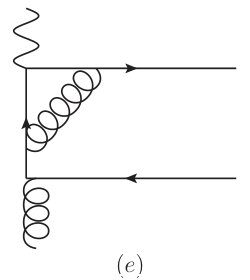
Next we discuss the IR property of one-loop amplitude. The complete amplitude is very complicated, but the IR divergent part can be shown to be simple and proportional to tree level amplitude. Here IR divergences include soft and collinear ones. These divergences can appear only in Fig.9(a,b,c,f,i). Our observation is the loop integrals with IR divergence can be expressed through three basic scalar loop integrals. Fig.9(a) contains only soft divergence, which is caused by the soft gluon exchange between the two quarks. Such soft divergence is contained in following integral,

IBox−a(0)(k1,k2)=∫l1[l2+i​ϵ]​[(l−k2)2−m2+i​ϵ]​[(l+p−k2)2−m2+i​ϵ]​[(l+k1)2−m2+i​ϵ],∫l=∫dn​l(2​π)n.\displaystyle I_{\text{Box}-a}^{(0)}(k_{1},k_{2})=\int_{l}\frac{1}{[l^{2}+i\epsilon][(l-k_{2})^{2}-m^{2}+i\epsilon][(l+p-k_{2})^{2}-m^{2}+i\epsilon][(l+k_{1})^{2}-m^{2}+i\epsilon]},\hskip 14.22636pt\int_{l}=\int\frac{d^{n}l}{(2\pi)^{n}}. (53)

The soft divergence of such box integral can be expressed through scalar triangle integrals[27]. In soft region with lμ=(l+,l−,l⟂μ)∼Q⁡(λ,λ,λ)l^{\mu}=(l^{+},l^{-},l_{\perp}^{\mu})\sim Q(\lambda,\lambda,\lambda), (l+p−k2)2−m2(l+p-k_{2})^{2}-m^{2} is offshell. Thus setting l=0l=0 in this propagator does not affect the IR divergence. This off-shell propagator can be decomposed as

1(l+p−k2)2−m2=1(p−k2)2−m2+l2−2​l⋅k2+2​l⋅p2​p⋅k2​[(l+p−k2)2−m2].\displaystyle\frac{1}{(l+p-k_{2})^{2}-m^{2}}=\frac{1}{(p-k_{2})^{2}-m^{2}}+\frac{l^{2}-2l\cdot k_{2}+2l\cdot p}{2p\cdot k_{2}[(l+p-k_{2})^{2}-m^{2}]}. (54)

The second term gives IR finite contribution. Then,

IBox−a(0)​(k1,k2)=\displaystyle I_{\text{Box}-a}^{(0)}(k_{1},k_{2})= 1−2p⋅k2​CTri​1​(s1)+DBox​1​(t1,u1),\displaystyle\frac{1}{-2p\cdot k_{2}}\text{CTri}1(s_{1})+\text{DBox}1(t_{1},u_{1}),
CTri​1​(s1)=\displaystyle\text{CTri}1(s_{1})= ∫l1(l2+i​ϵ)​[(l−k2)2−m2+i​ϵ]​[(l+k1)2−m2+i​ϵ].\displaystyle\int_{l}\frac{1}{(l^{2}+i\epsilon)[(l-k_{2})^{2}-m^{2}+i\epsilon][(l+k_{1})^{2}-m^{2}+i\epsilon]}. (55)

All soft divergence of the box integral now is contained in the triangle integral CTri​1​(s1)\text{CTri}1(s_{1}). Note that CTri​1​(s1)\text{CTri}1(s_{1}) is symmetric in k1k_{1}, k2k_{2} or t1,u1t_{1},u_{1}. By exchanging k1k_{1} and k2k_{2}, the soft divergence of Fig.9(b) is obtained. After some simplifications the sum of the divergent parts of Fig.9(a,b) is

ℳαμ|a+bI​R≐\displaystyle\left.\mathcal{M}^{\mu}_{\alpha}\right|_{a+b}^{IR}\doteq −i​g2​(CA−2​CF)​(2​k1⋅k2)​CTri​1​(s1)​{−g​Ta​12​p⋅k2​(u¯​(k1)​γμ​p̸​γα​v​(k2)−2​k2​α​u¯​(k1)​γμ​v​(k2))−(k1↔k2)}.\displaystyle-ig^{2}(C_{A}-2C_{F})(2k_{1}\cdot k_{2})\text{CTri}1(s_{1})\left\{-gT^{a}\frac{1}{2p\cdot k_{2}}(\bar{u}(k_{1})\gamma^{\mu}\not{p}\gamma_{\alpha}v(k_{2})-2k_{2\alpha}\bar{u}(k_{1})\gamma^{\mu}v(k_{2}))-(k_{1}\leftrightarrow k_{2})\right\}. (56)

The quantity in {⋯}\{\cdots\} is rightly the tree level amplitude. Hence,

ℳαμ|a+bI​R≐\displaystyle\left.\mathcal{M}^{\mu}_{\alpha}\right|_{a+b}^{IR}\doteq −i​g2​(CA−2​CF)​(2​k1⋅k2)​CTri​1​(s1)​ℳαμ⁡(0).\displaystyle-ig^{2}(C_{A}-2C_{F})(2k_{1}\cdot k_{2})\text{CTri}1(s_{1})\mathcal{M}^{\mu(0)}_{\alpha}. (57)

For Fig.9(c), both soft and collinear divergences are contained in the loop integral, and the overlap of these two divergences makes the extraction of IR part nontrivial. The divergent loop integrals for this diagram are

IBox−c(0,1,2)=\displaystyle I_{\text{Box}-c}^{(0,1,2)}= ∫l{1,(l+/p+),(l+/p+)2}D0​D1​D2​D3,\displaystyle\int_{l}\frac{\{1,(l^{+}/p^{+}),(l^{+}/p^{+})^{2}\}}{D_{0}D_{1}D_{2}D_{3}}, (58)

with

D0=l2,D1=(l+p)2,D2=(l+p−k2)2−m2,D3=(l+k1)2−m2.\displaystyle D_{0}=l^{2},\ D_{1}=(l+p)^{2},\ D_{2}=(l+p-k_{2})^{2}-m^{2},\ D_{3}=(l+k_{1})^{2}-m^{2}. (59)

In IBox​c(0)I_{\text{Box}c}^{(0)}, collinear divergence comes from the region where lμl^{\mu} is collinear to pμp^{\mu}, while soft divergence comes from two regions: one is lμl^{\mu} is soft, the other is (p−l)μ(p-l)^{\mu} is soft. In IBox​c(1,2)I_{\text{Box}c}^{(1,2)}, collinear divergences come from the same region as IBox​c(0)I_{\text{Box}c}^{(0)}, but the soft divergence only comes from the region where (p−l)μ(p-l)^{\mu} is soft. Note that the integral with (l+)3(l^{+})^{3} in the integrand is absent in the amplitude, although this integral is also IR divergent.

As we will show, the divergent part of Box-c can still be expressed through triangle integrals. First, setting l=0l=0 in D2D_{2} gives

IBox−c(0)≐\displaystyle I_{\text{Box}-c}^{(0)}\doteq −12​p⋅k2∫l1D0​D1​D3−1p⋅k2∫ll⋅k2D0​D1​D2​D3,\displaystyle-\frac{1}{2p\cdot k_{2}}\int_{l}\frac{1}{D_{0}D_{1}D_{3}}-\frac{1}{p\cdot k_{2}}\int_{l}\frac{l\cdot k_{2}}{D_{0}D_{1}D_{2}D_{3}}, (60)

where ≐\doteq means the equality holds up to IR finite corrections. Now l⋅k2=l+​k2−+l−​k2++l⟂⋅k2l\cdot k_{2}=l^{+}k_{2}^{-}+l^{-}k_{2}^{+}+l_{\perp}\cdot k_{2}, but l−l^{-} and l⟂l_{\perp} are suppressed by λ\lambda or λ2\lambda^{2} in soft or collinear regions, so, l−l^{-} and l⟂l_{\perp} can be dropped. Then

1p⋅k2​∫ll⋅k2D0​D1​D2​D3≐1p+​∫ll+D0​D1​D2​D3≐1p⋅q​∫ll⋅qD0​D1​D2​D3≐1p⋅q​∫ll⋅(k1+k2)D0​D1​D2​D3\displaystyle\frac{1}{p\cdot k_{2}}\int_{l}\frac{l\cdot k_{2}}{D_{0}D_{1}D_{2}D_{3}}\doteq\frac{1}{p^{+}}\int_{l}\frac{l^{+}}{D_{0}D_{1}D_{2}D_{3}}\doteq\frac{1}{p\cdot q}\int_{l}\frac{l\cdot q}{D_{0}D_{1}D_{2}D_{3}}\doteq\frac{1}{p\cdot q}\int_{l}\frac{l\cdot(k_{1}+k_{2})}{D_{0}D_{1}D_{2}D_{3}}
=\displaystyle= 1p⋅q​∫lD3−D0+D1−D2−2​k2⋅pD0​D1​D2​D3,\displaystyle\frac{1}{p\cdot q}\int_{l}\frac{D_{3}-D_{0}+D_{1}-D_{2}-2k_{2}\cdot p}{D_{0}D_{1}D_{2}D_{3}}, (61)

where we have used qμ=−pμ+k1μ+k2μq^{\mu}=-p^{\mu}+k_{1}^{\mu}+k_{2}^{\mu}. Now D0,1D_{0,1} in the numerator above can be dropped, because they are suppressed by λ\lambda or λ2\lambda^{2} in soft or collinear regions. Then, substituting this result back to eq.(60) one gets

IBox−c(0)=\displaystyle I_{\text{Box}-c}^{(0)}= −12​p⋅k2∫l1D0​D1​D3−12​p⋅k1∫l1D0​D1​D2+DBox2[t1,u1].\displaystyle-\frac{1}{2p\cdot k_{2}}\int_{l}\frac{1}{D_{0}D_{1}D_{3}}-\frac{1}{2p\cdot k_{1}}\int_{l}\frac{1}{D_{0}D_{1}D_{2}}+\text{DBox2}[t_{1},u_{1}]. (62)

In this way we express the IR part of Box-c through two triangle integrals. As expected, this expression is symmetric in k1,k2k_{1},k_{2}. In the above we have also defined the finite part of this box integral as DBox2​[t1,u1]\text{DBox2}[t_{1},u_{1}].

Similarly, one can show

IBox−c(1)≐\displaystyle I_{\text{Box}-c}^{(1)}\doteq 12​p⋅k1∫l1D0​D1​D2,IBox−c(2)≐−12​p⋅k1∫l1D0​D1​D2−14​p⋅k1​p⋅k2∫l1D0​D1.\displaystyle\frac{1}{2p\cdot k_{1}}\int_{l}\frac{1}{D_{0}D_{1}D_{2}},\hskip 28.45274ptI_{\text{Box}-c}^{(2)}\doteq-\frac{1}{2p\cdot k_{1}}\int_{l}\frac{1}{D_{0}D_{1}D_{2}}-\frac{1}{4p\cdot k_{1}p\cdot k_{2}}\int_{l}\frac{1}{D_{0}D_{1}}. (63)

With the same method, the extraction of IR divergence from the triangle diagrams Fig.9(f) becomes easy, and the results are

ITri−f(0)=\displaystyle I_{\text{Tri}-f}^{(0)}= ∫l1l2​(l+p)2​[(l+k2)2−m2]=∫l1l2​(l+p)2​[(l+p−k2)2−m2]=∫l1D0​D1​D2,\displaystyle\int_{l}\frac{1}{l^{2}(l+p)^{2}[(l+k_{2})^{2}-m^{2}]}=\int_{l}\frac{1}{l^{2}(l+p)^{2}[(l+p-k_{2})^{2}-m^{2}]}=\int_{l}\frac{1}{D_{0}D_{1}D_{2}},
ITri−f(1)=\displaystyle I_{\text{Tri}-f}^{(1)}= ∫l(l+/p+)l2​(l+p)2​[(l+k2)2−m2]≐12​p⋅k2​∫l1D0​D1.\displaystyle\int_{l}\frac{(l^{+}/p^{+})}{l^{2}(l+p)^{2}[(l+k_{2})^{2}-m^{2}]}\doteq\frac{1}{2p\cdot k_{2}}\int_{l}\frac{1}{D_{0}D_{1}}. (64)

The integrals with (l+)2(l^{+})^{2} or (l+)3(l^{+})^{3} do not appear in the amplitude, although they are divergent. Other integrals are IR finite for this triangle diagram. By exchanging k1,k2k_{1},k_{2} the divergent part of Fig.9(i) can be obtained.

With the obtained IR divergence, the amplitude from Fig.9(a,b,c,f,i) can be expressed through four basic scalar integrals J01,J012,J013J_{01},J_{012},J_{013} and CTri1​(s1)\text{CTri1}(s_{1}). After a lengthy calculation the result is put into a very neat form, which is proportional to tree level amplitude! Besides, the self-energy corrections to external fermion lines also contain IR divergence. Then, the complete IR divergent part of the amplitude is

ℳαμ⁡(1)|I​R=\displaystyle\left.\mathcal{M}^{\mu(1)}_{\alpha}\right|_{IR}= WI​R​ℳαμ⁡(0),\displaystyle W_{IR}\mathcal{M}^{\mu(0)}_{\alpha},
WI​R=\displaystyle W_{IR}= (Z2−1)−i​g2​(CA−2​CF)​(2​k1⋅k2)​CTri​1​(s1)−i​g2​CA​(2​p⋅k1​J013+2​p⋅k2​J012+J01),\displaystyle(Z_{2}-1)-ig^{2}(C_{A}-2C_{F})(2k_{1}\cdot k_{2})\text{CTri}1(s_{1})-ig^{2}C_{A}(2p\cdot k_{1}J_{013}+2p\cdot k_{2}J_{012}+J_{01}), (65)

with

J012=∫l1D0​D1​D2,J013=∫l1D0​D1​D3,J01=∫l1D0​D1.\displaystyle J_{012}=\int_{l}\frac{1}{D_{0}D_{1}D_{2}},\ J_{013}=\int_{l}\frac{1}{D_{0}D_{1}D_{3}},\ J_{01}=\int_{l}\frac{1}{D_{0}D_{1}}. (66)

This is one of our main results. The derivation of this result is independent of the polarizations of external gluon, thus this result indicates the IR divergence, including soft and collinear ones, is spin independent. According to eq.(50), the IR divergence of hard part is

Hα​βμ​ν​(1)|I​R=2​Re​(WI​R)​Hα​βμ​ν​(0),\displaystyle\left.H^{\mu\nu(1)}_{\alpha\beta}\right|_{IR}=2\text{Re}(W_{IR})H^{\mu\nu(0)}_{\alpha\beta}, (67)

where the factor 22 indicates the contribution from conjugated diagrams.

Besides IR divergence, the hard part also contains UV divergence, which is subtracted by the counter terms of lagrangian. After the subtraction of UV divergence, the hard part gives a μ\mu dependence, with μ\mu the renormalization scale. We will separate the μ\mu dependence in the following.

Notice that the electro-magnetic current jμj^{\mu} in hadronic tensor is conserved, so, the UV divergence from vertex correction is cancelled by self-energy correction to fermions. This means the UV divergences of Fig.9(e,h) are cancelled by Fig.9(j,k). So, the sum of these four diagrams does not generate μ\mu dependence. Apart from the μ\mu dependence in wave function renormalization constant for fermions, i.e., Z2Z_{2}, the remaining μ\mu dependence can only come from Fig.9(d,f,g,i). The UV divergence of these diagrams reads

ℳαμ|d+g≐\displaystyle\left.\mathcal{M}^{\mu}_{\alpha}\right|_{d+g}\doteq −CA−2​CF2​αs​(4​π​μ2/Q2)ϵ/24​π​Γ​(ϵU​V2)​ℳαμ⁡(0),\displaystyle-\frac{C_{A}-2C_{F}}{2}\frac{\alpha_{s}(4\pi\mu^{2}/Q^{2})^{\epsilon/2}}{4\pi}\Gamma(\frac{\epsilon_{UV}}{2})\mathcal{M}^{\mu(0)}_{\alpha},
ℳαμ|f+i≐\displaystyle\left.\mathcal{M}^{\mu}_{\alpha}\right|_{f+i}\doteq 3​CA2​αs​(4​π​μ2/Q2)ϵ/24​π​Γ​(ϵU​V2)​ℳαμ⁡(0).\displaystyle\frac{3C_{A}}{2}\frac{\alpha_{s}(4\pi\mu^{2}/Q^{2})^{\epsilon/2}}{4\pi}\Gamma(\frac{\epsilon_{UV}}{2})\mathcal{M}^{\mu(0)}_{\alpha}. (68)

With the μ\mu dependence from Z2Z_{2}, the total μ\mu-dependence of the amplitude is

ℳαμ⁡(1)=\displaystyle\mathcal{M}^{\mu(1)}_{\alpha}= [−CA−2​CF2+3​CA2−CF]​αs4​π​ln⁡μ2Q2​ℳαμ⁡(0)+⋯,\displaystyle\left[-\frac{C_{A}-2C_{F}}{2}+\frac{3C_{A}}{2}-C_{F}\right]\frac{\alpha_{s}}{4\pi}\ln\frac{\mu^{2}}{Q^{2}}\mathcal{M}^{\mu(0)}_{\alpha}+\cdots, (69)

where ⋯\cdots represents μ\mu independent part.

With renormalization scale separated explicitly, the hard part can be written as

Hα​βμ​ν​(1)=H1​α​βμ​ν+H2​α​βμ​ν+H3​α​βμ​ν,\displaystyle H^{\mu\nu(1)}_{\alpha\beta}=H^{\mu\nu}_{1\alpha\beta}+H^{\mu\nu}_{2\alpha\beta}+H^{\mu\nu}_{3\alpha\beta}, (70)

with

H1​α​βμ​ν=\displaystyle H^{\mu\nu}_{1\alpha\beta}= 2​Re​(WI​R)​Hα​βμ​ν​(0)|μ2=Q2,\displaystyle\left.2\text{Re}(W_{IR})H^{\mu\nu(0)}_{\alpha\beta}\right|_{\mu^{2}=Q^{2}},
H2​α​βμ​ν=\displaystyle H^{\mu\nu}_{2\alpha\beta}= (Hα​βμ​ν​(1)−2​Re​(WI​R)​Hα​βμ​ν​(0))μ2=Q2,\displaystyle\left(H^{\mu\nu(1)}_{\alpha\beta}-2\text{Re}(W_{IR})H^{\mu\nu(0)}_{\alpha\beta}\right)_{\mu^{2}=Q^{2}},
H3​α​βμ​ν=\displaystyle H^{\mu\nu}_{3\alpha\beta}= 2​αs4​π​CA​ln⁡μ2Q2​Hα​βμ​ν​(0),\displaystyle 2\frac{\alpha_{s}}{4\pi}C_{A}\ln\frac{\mu^{2}}{Q^{2}}H^{\mu\nu(0)}_{\alpha\beta}, (71)

where we have chosen the reference scale of μ2\mu^{2} as Q2Q^{2} so that H3H_{3} is definite. These three parts make the structure of one-loop virtual correction to hadronic tensor clear.

At last, it should be pointed out that only in pole mass scheme, the μ\mu dependence of Fig.9(j,k) is proportional to tree level amplitude. In pole mass scheme the mass counter term in lagrangian is chosen so that renormalized fermion self-energy ΣR​(p~,m)=0\Sigma_{R}(\not{\tilde{p}},m)=0 when p~=m\not{\tilde{p}}=m. Then the renormalized self-energy is written as

ΣR​(p̸~,m)=\displaystyle\Sigma_{R}(\tilde{\not{p}},m)= −αs4​π​CF​ln⁡μ2Q2​(p̸~−m)+αs4​π​CF​(p̸~​Bv​(−p~2m2,Q2m2)+m​Bm​(−p~2m2,Q2m2)),\displaystyle-\frac{\alpha_{s}}{4\pi}C_{F}\ln\frac{\mu^{2}}{Q^{2}}(\tilde{\not{p}}-m)+\frac{\alpha_{s}}{4\pi}C_{F}\left(\tilde{\not{p}}B_{v}(\frac{-\tilde{p}^{2}}{m^{2}},\frac{Q^{2}}{m^{2}})+mB_{m}(\frac{-\tilde{p}^{2}}{m^{2}},\frac{Q^{2}}{m^{2}})\right), (72)

with

Bv​(z,τ)\displaystyle B_{v}(z,\tau) =∫01d​x​x​ln⁡(x​z+1)−ln⁡τ=(2−z)​z−2​(1−z2)​ln⁡(1+z)4​z2−ln⁡τ,\displaystyle=\int_{0}^{1}dxx\ln(xz+1)-\ln\tau=\frac{(2-z)z-2(1-z^{2})\ln(1+z)}{4z^{2}}-\ln\tau,
Bm​(z,τ)\displaystyle B_{m}(z,\tau) =−2−4​∫01d​x​ln⁡(x​z+1)+ln⁡τ=2−4​(1+z)z​ln⁡(1+z)+ln⁡τ.\displaystyle=-2-4\int_{0}^{1}dx\ln(xz+1)+\ln\tau=2-\frac{4(1+z)}{z}\ln(1+z)+\ln\tau. (73)

From the structure of self-energy correction, ln⁡μ\ln\mu part is proportional to tree diagrams. As stated before this μ\mu dependence is cancelled by that of Fig.9(e,h). This is an advantage of pole mass scheme.

IV.3 Subtraction and finite hard coefficients

According to our subtraction scheme in eq.(39) and results in eq.(47,48,49,67), the finite hard coefficient is given by

Hα​βμ​ν​(1)|f​i​n​i​t​e=\displaystyle\left.H^{\mu\nu(1)}_{\alpha\beta}\right|_{finite}= Hα​βμ​ν​(1)−2​R​e​[WΦ+WS​Q+WS]​Hα​βμ​ν​(0)\displaystyle H^{\mu\nu(1)}_{\alpha\beta}-2Re[W_{\Phi}+W_{SQ}+W_{S}]H^{\mu\nu(0)}_{\alpha\beta}
=\displaystyle= 2​R​e​[(WI​R+CF​αs4​π​ln⁡μ2Q2−CA​αs4​π​ln⁡μ2Q2)−WΦ−WS​Q−WS]​Hα​βμ​ν​(0)+H3​α​βμ​ν+H2​α​βμ​ν,\displaystyle 2Re\left[\left(W_{IR}+C_{F}\frac{\alpha_{s}}{4\pi}\ln\frac{\mu^{2}}{Q^{2}}-C_{A}\frac{\alpha_{s}}{4\pi}\ln\frac{\mu^{2}}{Q^{2}}\right)-W_{\Phi}-W_{SQ}-W_{S}\right]H^{\mu\nu(0)}_{\alpha\beta}+H^{\mu\nu}_{3\alpha\beta}+H^{\mu\nu}_{2\alpha\beta}, (74)

where we have used the fact

WI​R|μ2=Q2=WI​R+CF​αs4​π​ln⁡μ2Q2−CA​αs4​π​ln⁡μ2Q2,\displaystyle W_{IR}|_{\mu^{2}=Q^{2}}=W_{IR}+C_{F}\frac{\alpha_{s}}{4\pi}\ln\frac{\mu^{2}}{Q^{2}}-C_{A}\frac{\alpha_{s}}{4\pi}\ln\frac{\mu^{2}}{Q^{2}}, (75)

and the ln⁡μ2\ln\mu^{2} is from Z2Z_{2} and J01J_{01}.

The explicit expression of IR divergent scalar loop integrals are calculated by standard Feynman parametrization. One can also find general expressions in e.g. [27],[28] and then continue the result into DIS region. Generally, the result in DIS region is very simple. For completeness we list the result of these integrals here as

CTri​1​(s1)=\displaystyle\text{CTri}1(s_{1})= −i16​π2Rϵ1s12​ρ12{−2ϵlnc12+(1−lnQ2s12)lnc12+12ln2c12\displaystyle-\frac{i}{16\pi^{2}}R_{\epsilon}\frac{1}{s_{12}\rho_{12}}\left\{-\frac{2}{\epsilon}\ln c_{12}+(1-\ln\frac{Q^{2}}{s_{12}})\ln c_{12}+\frac{1}{2}\ln^{2}c_{12}\right.
+2lnρ12lnc12+2​π23+2Li2(c12)},Rϵ=(4​π​μ2/Q2)ϵ/2Γ⁡(2−ϵ/2),\displaystyle\left.+2\ln\rho_{12}\ln c_{12}+\frac{2\pi^{2}}{3}+2Li_{2}(c_{12})\right\},\hskip 14.22636ptR_{\epsilon}=\frac{(4\pi\mu^{2}/Q^{2})^{\epsilon/2}}{\Gamma(2-\epsilon/2)}, (76)

and

J013=\displaystyle J_{013}= i16​π2​Rϵ​1Q2​y13​2ϵ2​[1−ϵ2+ϵ2​ln⁡rby132+ϵ22​(−12​ln⁡rby132+14​ln2​rby132+π212+L​i2​(rb+y13rb))],\displaystyle\frac{i}{16\pi^{2}}R_{\epsilon}\frac{1}{Q^{2}y_{13}}\frac{2}{\epsilon^{2}}\left[1-\frac{\epsilon}{2}+\frac{\epsilon}{2}\ln\frac{r_{b}}{y_{13}^{2}}+\frac{\epsilon^{2}}{2}\left(-\frac{1}{2}\ln\frac{r_{b}}{y_{13}^{2}}+\frac{1}{4}\ln^{2}\frac{r_{b}}{y_{13}^{2}}+\frac{\pi^{2}}{12}+Li_{2}(\frac{r_{b}+y_{13}}{r_{b}})\right)\right],
J012=\displaystyle J_{012}= J013|y13→y23,\displaystyle\left.J_{013}\right|_{y_{13}\to y_{23}},
J01=\displaystyle J_{01}= i16​π2​(2ϵU​V−2ϵI​R),\displaystyle\frac{i}{16\pi^{2}}\left(\frac{2}{\epsilon_{UV}}-\frac{2}{\epsilon_{IR}}\right), (77)

where

s12=(k1+k2)2,ρ12=1−4​m2s12,c12=ln⁡1−ρ121+ρ12,\displaystyle s_{12}=(k_{1}+k_{2})^{2},\ \rho_{12}=\sqrt{1-\frac{4m^{2}}{s_{12}}},\ c_{12}=\ln\frac{1-\rho_{12}}{1+\rho_{12}}, (78)

and

y13=2​p⋅k1q2,y23=2​p⋅k2q2,y12=−2​k1⋅k2q2,rb=−m2q2.\displaystyle y_{13}=\frac{2p\cdot k_{1}}{q^{2}},\ y_{23}=\frac{2p\cdot k_{2}}{q^{2}},\ y_{12}=-\frac{2k_{1}\cdot k_{2}}{q^{2}},\ r_{b}=-\frac{m^{2}}{q^{2}}. (79)

In DIS region, y13,y23<0y_{13},y_{23}<0 and y12,rb>0y_{12},r_{b}>0. In these integrals we have ignored all absorptive parts.

With these integrals, the explicit WI​RW_{IR} can be obtained as

WI​R=\displaystyle W_{IR}= (Z2−1)−(CA−2CF)αs4​πRϵ1+ρ1222​ρ12{−2ϵlnc12+(1−lnQ2s12)lnc12+12ln2c12\displaystyle(Z_{2}-1)-(C_{A}-2C_{F})\frac{\alpha_{s}}{4\pi}R_{\epsilon}\frac{1+\rho_{12}^{2}}{2\rho_{12}}\left\{-\frac{2}{\epsilon}\ln c_{12}+(1-\ln\frac{Q^{2}}{s_{12}})\ln c_{12}+\frac{1}{2}\ln^{2}c_{12}\right.
+2lnρ12lnc12+2​π23+2Li2(c12)}\displaystyle\left.+2\ln\rho_{12}\ln c_{12}+\frac{2\pi^{2}}{3}+2Li_{2}(c_{12})\right\}
−CAαs4​πRϵ{4ϵ2−2ϵ+2ϵlnrby13​y23−lnrby13​y23\displaystyle-C_{A}\frac{\alpha_{s}}{4\pi}R_{\epsilon}\left\{\frac{4}{\epsilon^{2}}-\frac{2}{\epsilon}+\frac{2}{\epsilon}\ln\frac{r_{b}}{y_{13}y_{23}}-\ln\frac{r_{b}}{y_{13}y_{23}}\right.
+π26+14ln2rby132+14ln2rby232+Li2(rb+y13rb)+Li2(rb+y23rb)}\displaystyle\left.+\frac{\pi^{2}}{6}+\frac{1}{4}\ln^{2}\frac{r_{b}}{y_{13}^{2}}+\frac{1}{4}\ln^{2}\frac{r_{b}}{y_{23}^{2}}+Li_{2}(\frac{r_{b}+y_{13}}{r_{b}})+Li_{2}(\frac{r_{b}+y_{23}}{r_{b}})\right\}
+CA​αs4​π​(2ϵU​V−2ϵI​R).\displaystyle+C_{A}\frac{\alpha_{s}}{4\pi}\left(\frac{2}{\epsilon_{UV}}-\frac{2}{\epsilon_{IR}}\right). (80)

The expression of WΦW_{\Phi} has been given by eq.(47), then we have

WI​R−WΦ=\displaystyle W_{IR}-W_{\Phi}= (Z2−Zv1/2)−(CA−2CF)αs4​πRϵ1+ρ1222​ρ12{−2ϵlnc12+(1−lnQ2s12)lnc12+12ln2c12\displaystyle(Z_{2}-Z_{v}^{1/2})-(C_{A}-2C_{F})\frac{\alpha_{s}}{4\pi}R_{\epsilon}\frac{1+\rho_{12}^{2}}{2\rho_{12}}\left\{-\frac{2}{\epsilon}\ln c_{12}+(1-\ln\frac{Q^{2}}{s_{12}})\ln c_{12}+\frac{1}{2}\ln^{2}c_{12}\right.
+2lnρ12lnc12+2​π23+2Li2(c12)}\displaystyle\left.+2\ln\rho_{12}\ln c_{12}+\frac{2\pi^{2}}{3}+2Li_{2}(c_{12})\right\}
−CAαs4​πRϵ{(2ϵ−1)ln(v⋅v~)2v2​v1⋅v~​v2⋅v~−π26+14ln2rby132+14ln2rby232−12ln2Q2ζ2\displaystyle-C_{A}\frac{\alpha_{s}}{4\pi}R_{\epsilon}\left\{(\frac{2}{\epsilon}-1)\ln\frac{(v\cdot\tilde{v})^{2}}{v^{2}v_{1}\cdot\tilde{v}v_{2}\cdot\tilde{v}}-\frac{\pi^{2}}{6}+\frac{1}{4}\ln^{2}\frac{r_{b}}{y_{13}^{2}}+\frac{1}{4}\ln^{2}\frac{r_{b}}{y_{23}^{2}}-\frac{1}{2}\ln^{2}\frac{Q^{2}}{\zeta^{2}}\right.
+Li2(rb+y13rb)+Li2(rb+y23rb)}.\displaystyle\left.+Li_{2}(\frac{r_{b}+y_{13}}{r_{b}})+Li_{2}(\frac{r_{b}+y_{23}}{r_{b}})\right\}. (81)

It can be seen the IR divergence from hard part cannot be subtracted by the correction to gluon TMDPDF alone. The TMD formula without soft factors must be wrong. At one-loop level, the two soft factors have been calculated in eq.(48) and eq.(49). We have

WS​Q+WS=\displaystyle W_{SQ}+W_{S}= (Zv1​Zv2​Zv~−Zv​Zv~)\displaystyle(\sqrt{Z_{v_{1}}Z_{v_{2}}Z_{\tilde{v}}}-\sqrt{Z_{v}Z_{\tilde{v}}})
−αs4​π​(1ϵU​V−1ϵI​R)​[2​CA​ln⁡v2​v1⋅v~​v2⋅v~(v⋅v~)2+(CA−2​CF)​1+ρ122ρ12​ln⁡1−ρ121+ρ12].\displaystyle-\frac{\alpha_{s}}{4\pi}\left(\frac{1}{\epsilon_{UV}}-\frac{1}{\epsilon_{IR}}\right)\left[2C_{A}\ln\frac{v^{2}v_{1}\cdot\tilde{v}v_{2}\cdot\tilde{v}}{(v\cdot\tilde{v})^{2}}+(C_{A}-2C_{F})\frac{1+\rho_{12}^{2}}{\rho_{12}}\ln\frac{1-\rho_{12}}{1+\rho_{12}}\right]. (82)

Now it is very clear that the difference between WI​R−WΦW_{IR}-W_{\Phi} and WS​Q+WSW_{SQ}+W_{S} is IR finite, i.e.,

(WI​R−WΦ)−(WS​Q+WS)\displaystyle(W_{IR}-W_{\Phi})-(W_{SQ}+W_{S})
=\displaystyle= −αs4​π​CF​(4+3​ln⁡μ2m2)\displaystyle-\frac{\alpha_{s}}{4\pi}C_{F}(4+3\ln\frac{\mu^{2}}{m^{2}})
−(CA−2CF)αs4​π1+ρ1222​ρ12{−lnμ2Q2lnc12+(1−lnQ2s12)lnc12+12ln2c12\displaystyle-(C_{A}-2C_{F})\frac{\alpha_{s}}{4\pi}\frac{1+\rho_{12}^{2}}{2\rho_{12}}\left\{-\ln\frac{\mu^{2}}{Q^{2}}\ln c_{12}+(1-\ln\frac{Q^{2}}{s_{12}})\ln c_{12}+\frac{1}{2}\ln^{2}c_{12}\right.
+2lnρ12lnc12+2​π23+2Li2(c12)}\displaystyle\left.+2\ln\rho_{12}\ln c_{12}+\frac{2\pi^{2}}{3}+2Li_{2}(c_{12})\right\}
−CAαs4​π{(lnμ2Q2−1)ln(v⋅v~)2v2​v1⋅v~​v2⋅v~−π26+14ln2rby132+14ln2rby232−12ln2Q2ζ2\displaystyle-C_{A}\frac{\alpha_{s}}{4\pi}\left\{(\ln\frac{\mu^{2}}{Q^{2}}-1)\ln\frac{(v\cdot\tilde{v})^{2}}{v^{2}v_{1}\cdot\tilde{v}v_{2}\cdot\tilde{v}}-\frac{\pi^{2}}{6}+\frac{1}{4}\ln^{2}\frac{r_{b}}{y_{13}^{2}}+\frac{1}{4}\ln^{2}\frac{r_{b}}{y_{23}^{2}}-\frac{1}{2}\ln^{2}\frac{Q^{2}}{\zeta^{2}}\right.
+Li2(rb+y13rb)+Li2(rb+y23rb)},\displaystyle\left.+Li_{2}(\frac{r_{b}+y_{13}}{r_{b}})+Li_{2}(\frac{r_{b}+y_{23}}{r_{b}})\right\}, (83)

In this result, the UV counter terms for gluon TMDPDF and soft factors have been added and the scale μ\mu is for UV renormalization. In eq.(83) the first line in the equality is given by wave function renormalization, that is,

(WI​R−WΦ)−(WS​Q+WS)⊃Z2−Zv1​Zv2.\displaystyle(W_{IR}-W_{\Phi})-(W_{SQ}+W_{S})\supset Z_{2}-\sqrt{Z_{v_{1}}Z_{v_{2}}}. (84)

After UV divergences are removed the wave function renormalization constants are

Z2=\displaystyle Z_{2}= 1−αs4​π​CF​ln⁡μ2Q2−αs2​π​CF​(2ϵI​R−γE+2+ln⁡4​π+32​ln⁡Q2m2+ln⁡μI​R2Q2),\displaystyle 1-\frac{\alpha_{s}}{4\pi}C_{F}\ln\frac{\mu^{2}}{Q^{2}}-\frac{\alpha_{s}}{2\pi}C_{F}\left(\frac{2}{\epsilon_{IR}}-\gamma_{E}+2+\ln 4\pi+\frac{3}{2}\ln\frac{Q^{2}}{m^{2}}+\ln\frac{\mu_{IR}^{2}}{Q^{2}}\right),
Zv1=Zv2=\displaystyle Z_{v_{1}}=Z_{v_{2}}= 1+αs2​π​CF​(2ϵU​V−2ϵI​R)+c.t.\displaystyle 1+\frac{\alpha_{s}}{2\pi}C_{F}(\frac{2}{\epsilon_{UV}}-\frac{2}{\epsilon_{IR}})+\text{c.t.}
=\displaystyle= −αs2​π​CF​(2ϵI​R−γE+ln⁡4​π​μI​R2μ2).\displaystyle-\frac{\alpha_{s}}{2\pi}C_{F}(\frac{2}{\epsilon_{IR}}-\gamma_{E}+\ln\frac{4\pi\mu_{IR}^{2}}{\mu^{2}}). (85)

So,

Z2−Zv1​Zv2=−αs4​π​CF​(4+3​ln⁡μ2m2).\displaystyle Z_{2}-\sqrt{Z_{v_{1}}Z_{v_{2}}}=-\frac{\alpha_{s}}{4\pi}C_{F}(4+3\ln\frac{\mu^{2}}{m^{2}}). (86)

Now, substituting eq.(83) into eq.(74), the finite hard coefficient is

Hρ​τμ​ν​(1)|f​i​n​i​t​e=\displaystyle\left.H^{\mu\nu(1)}_{\rho\tau}\right|_{finite}= Wf​Hρ​τμ​ν​(0)+H2​ρ​τμ​ν,\displaystyle W_{f}H^{\mu\nu(0)}_{\rho\tau}+H^{\mu\nu}_{2\rho\tau},
Wf=\displaystyle W_{f}= 2{αs4​πlnμ2Q2[−CAln(v⋅v~)2v2​v~⋅v1​v~⋅v2−2CF+(CA−2CF)(1+ρ1222​ρ12ln1−ρ121+ρ12)]\displaystyle 2\left\{\frac{\alpha_{s}}{4\pi}\ln\frac{\mu^{2}}{Q^{2}}\left[-C_{A}\ln\frac{(v\cdot\tilde{v})^{2}}{v^{2}\tilde{v}\cdot v_{1}\tilde{v}\cdot v_{2}}-2C_{F}+(C_{A}-2C_{F})\left(\frac{1+\rho_{12}^{2}}{2\rho_{12}}\ln\frac{1-\rho_{12}}{1+\rho_{12}}\right)\right]\right.
+(WI​R−WΦ−WS​Q−WS)μ2=Q2}\displaystyle\left.+\left(W_{IR}-W_{\Phi}-W_{SQ}-W_{S}\right)_{\mu^{2}=Q^{2}}\right\}
=\displaystyle= αs2​π​ln⁡μ2Q2​[−CA​ln⁡(v⋅v~)2v2​v~⋅v1​v~⋅v2−2​CF+(CA−2​CF)​(1+ρ1222​ρ12​ln⁡1−ρ121+ρ12)]\displaystyle\frac{\alpha_{s}}{2\pi}\ln\frac{\mu^{2}}{Q^{2}}\left[-C_{A}\ln\frac{(v\cdot\tilde{v})^{2}}{v^{2}\tilde{v}\cdot v_{1}\tilde{v}\cdot v_{2}}-2C_{F}+(C_{A}-2C_{F})\left(\frac{1+\rho_{12}^{2}}{2\rho_{12}}\ln\frac{1-\rho_{12}}{1+\rho_{12}}\right)\right]
−(CA−2​CF)​αs2​π​1+ρ1222​ρ12​[(1−ln⁡Q2s12)​ln⁡c12+12​ln2​c12+2​ln⁡ρ12​ln​c12+2​π23+2​L​i2​(c12)]\displaystyle-(C_{A}-2C_{F})\frac{\alpha_{s}}{2\pi}\frac{1+\rho_{12}^{2}}{2\rho_{12}}\left[(1-\ln\frac{Q^{2}}{s_{12}})\ln c_{12}+\frac{1}{2}\ln^{2}c_{12}+2\ln\rho_{12}\ln c_{12}+\frac{2\pi^{2}}{3}+2Li_{2}(c_{12})\right]
−CA​αs2​π​[−π26+14​ln2​rby132+14​ln2​rby232−12​ln2​Q2ζ2+L​i2​(rb+y13rb)+L​i2​(rb+y23rb)]\displaystyle-C_{A}\frac{\alpha_{s}}{2\pi}\left[-\frac{\pi^{2}}{6}+\frac{1}{4}\ln^{2}\frac{r_{b}}{y_{13}^{2}}+\frac{1}{4}\ln^{2}\frac{r_{b}}{y_{23}^{2}}-\frac{1}{2}\ln^{2}\frac{Q^{2}}{\zeta^{2}}+Li_{2}(\frac{r_{b}+y_{13}}{r_{b}})+Li_{2}(\frac{r_{b}+y_{23}}{r_{b}})\right]
−αs2​π​CF​(4+3​ln⁡Q2m2).\displaystyle-\frac{\alpha_{s}}{2\pi}C_{F}(4+3\ln\frac{Q^{2}}{m^{2}}). (87)

Moreover, our decomposition for hard coefficient in eq.(23) is effective to all orders of αs\alpha_{s} if only virtual correction is involved. So, H2​α​βμ​νH^{\mu\nu}_{2\alpha\beta} can still be projected into 10 scalar hard coefficients H2i​jH_{2}^{ij} as we done for Hα​βμ​ν​(0)H^{\mu\nu(0)}_{\alpha\beta}. There will be no other new tensor structure in higher order correction. That is,

Hf​i​n​i​t​e(1)​i​j=Wf​H(0)​i​j+H2i​j,\displaystyle H^{(1)ij}_{finite}=W_{f}H^{(0)ij}+H_{2}^{ij}, (88)

with the projection in eq.(23). There is not any new tensor structure appearing in higher order correction, since only virtual correction contributes. Eq.(87,88) is one of our main results. From the derivation, WI​RW_{IR} and WΦW_{\Phi} are independent of the polarizations of parton or gluon, so, WfW_{f} is the same to all gluon TMDPDFs, including those defined by polarized hadron as given in [1]. H2H_{2} depends on the polarizations of gluon, but it is IR finite and μ\mu independent. The finiteness of H2H_{2} is justified explicitly according to eq.(71). In our result, it is expressed through some basic IR finite scalar loop integrals, including box integrals DBox​1,2\text{DBox}1,2, triangle integrals CTri​3,4,5\text{CTri}3,4,5 and various bubble integrals b0b_{0}, BvB_{v} and BmB_{m}. These integrals are illustrated in Appendix..

In our result, the projected hard coefficients H2i​jH_{2}^{ij} according to eq.(23) are given in a mathematica file s​u​b​t​e​d​2.msubted2.m. These results are very lengthy and cannot be shown here. In s​u​b​t​e​d​2.msubted2.m these projected hard coefficients are stored as a list

{ξ1​H211,ξ2​H212,ξ3​H221,ξ4​H222,ξ5​H233,ξ6​H241,ξ7​H242,ξ8​H251,ξ9​H252,ξ10​H263},\displaystyle\{\xi_{1}H_{2}^{11},\xi_{2}H_{2}^{12},\xi_{3}H_{2}^{21},\xi_{4}H_{2}^{22},\xi_{5}H_{2}^{33},\xi_{6}H_{2}^{41},\xi_{7}H_{2}^{42},\xi_{8}H_{2}^{51},\xi_{9}H_{2}^{52},\xi_{10}H_{2}^{63}\}, (89)

with normalization factors

ξ1=\displaystyle\xi_{1}= ξ2=1gs4​Q2​|k1⟂|2,\displaystyle\xi_{2}=\frac{1}{g_{s}^{4}}Q^{2}|k_{1\perp}|^{2},
ξ3=\displaystyle\xi_{3}= ξ4=ξ5=−1gs4​2​Q​|k1⟂|3,\displaystyle\xi_{4}=\xi_{5}=-\frac{1}{g_{s}^{4}}2Q|k_{1\perp}|^{3},
ξ6=\displaystyle\xi_{6}= ξ7=ξ8=ξ9=ξ10=1gs4​2​|k1⟂|4.\displaystyle\xi_{7}=\xi_{8}=\xi_{9}=\xi_{10}=\frac{1}{g_{s}^{4}}2|k_{1\perp}|^{4}. (90)

All of these results are expressed through the invariants s1,t1,u1s_{1},t_{1},u_{1} and mm appearing in tree level result eq.(31). There are two color factors in the stored result, i.e.,

f⁡(N1)=T​r​(Ta​Tb​Ta​Tb)=1−Nc24​Nc,f⁡(N2)=T​r​(Ta​Ta​Tb​Tb)=(Nc2−1)24​Nc.\displaystyle f(N_{1})=Tr(T^{a}T^{b}T^{a}T^{b})=\frac{1-N_{c}^{2}}{4N_{c}},\ f(N_{2})=Tr(T^{a}T^{a}T^{b}T^{b})=\frac{(N_{c}^{2}-1)^{2}}{4N_{c}}. (91)

In the final part it is interesting to point out that our factorization formula eq.(37) associated with the finite hard part given by eq.(87) is μ\mu independent to order of αs2\alpha_{s}^{2}. This can be illustrated in the following. Because real correction is UV finite, μ\mu dependence is purely generated by virtual corrections. Then, the μ\mu dependence of SQ​(l⟂)S^{Q}(l_{\perp}) and S¯​(l⟂)\bar{S}(l_{\perp}) can be obtained from eq.(48) and eq.(49), respectively. They are

∂SQ​(l⟂)∂ln⁡μ2=\displaystyle\frac{\partial S^{Q}(l_{\perp})}{\partial\ln\mu^{2}}= αs2​π​[2​CF+CA−CA​ln⁡4​v1⋅v~​v2⋅v~v~2−(CA−2​CF)​1+ρ1222​ρ12​ln⁡1−ρ121+ρ12]​SQ​(l⟂),\displaystyle\frac{\alpha_{s}}{2\pi}\left[2C_{F}+C_{A}-C_{A}\ln\frac{4v_{1}\cdot\tilde{v}v_{2}\cdot\tilde{v}}{\tilde{v}^{2}}-(C_{A}-2C_{F})\frac{1+\rho_{12}^{2}}{2\rho_{12}}\ln\frac{1-\rho_{12}}{1+\rho_{12}}\right]S^{Q}(l_{\perp}),
∂S¯​(l⟂)∂ln⁡μ2=\displaystyle\frac{\partial\bar{S}(l_{\perp})}{\partial\ln\mu^{2}}= αs2​π​CA​[−2+ln⁡4​(v⋅v~)2v2​v~2]​S¯​(l⟂).\displaystyle\frac{\alpha_{s}}{2\pi}C_{A}\left[-2+\ln\frac{4(v\cdot\tilde{v})^{2}}{v^{2}\tilde{v}^{2}}\right]\bar{S}(l_{\perp}). (92)

For gluon TMDPDF, additional self-energy correction to gluon with momentum pp should be added into virtual correction. Of course, this correction does not affect the finite hard part, because it cancels the same gluon self-energy insertion in hard scattering for hadronic tensor. The wave function renormalization constant in Feynman gauge is

ZG=1−αs4​π​(23​NF−53​CA)​(2ϵU​V−γE+ln⁡4​π),\displaystyle Z_{G}=1-\frac{\alpha_{s}}{4\pi}\left(\frac{2}{3}N_{F}-\frac{5}{3}C_{A}\right)(\frac{2}{\epsilon_{UV}}-\gamma_{E}+\ln 4\pi), (93)

in M​S¯\overline{MS} scheme. Then, from eq.(47) we have

∂∂ln⁡μ2​Φα​β​(x,p⟂)=\displaystyle\frac{\partial}{\partial\ln\mu^{2}}\Phi^{\alpha\beta}(x,p_{\perp})= −αs4​π​[23​NF−53​CA−4​CA]​Φα​β​(x,p⟂).\displaystyle-\frac{\alpha_{s}}{4\pi}\left[\frac{2}{3}N_{F}-\frac{5}{3}C_{A}-4C_{A}\right]\Phi^{\alpha\beta}(x,p_{\perp}). (94)

Recall that tree level hard coefficients are proportional to αs\alpha_{s}, which has a μ\mu dependence

∂αs∂ln⁡μ2=β⁡(αs)=−αs24​π​(113​CA−23​NF).\displaystyle\frac{\partial\alpha_{s}}{\partial\ln\mu^{2}}=\beta(\alpha_{s})=-\frac{\alpha_{s}^{2}}{4\pi}\left(\frac{11}{3}C_{A}-\frac{2}{3}N_{F}\right). (95)

Now the hadronic tensor to 𝒪⁡(αs2)\mathcal{O}(\alpha_{s}^{2}) can be written as

Wμ​ν∝\displaystyle W^{\mu\nu}\propto αs​[1+αs2​π​ln⁡μ2Q2​(−CA​ln⁡(v⋅v~)2v2​v~⋅v1​v~⋅v2−2​CF+(CA−2​CF)​1+ρ1222​ρ12​ln⁡1−ρ121+ρ12)+⋯]\displaystyle\alpha_{s}\left[1+\frac{\alpha_{s}}{2\pi}\ln\frac{\mu^{2}}{Q^{2}}\left(-C_{A}\ln\frac{(v\cdot\tilde{v})^{2}}{v^{2}\tilde{v}\cdot v_{1}\tilde{v}\cdot v_{2}}-2C_{F}+(C_{A}-2C_{F})\frac{1+\rho_{12}^{2}}{2\rho_{12}}\ln\frac{1-\rho_{12}}{1+\rho_{12}}\right)+\cdots\right]
Φα​β​(x,p⟂)⊗SQ​(l1⟂)⊗S¯​(l2⟂),\displaystyle\Phi^{\alpha\beta}(x,p_{\perp})\otimes S^{Q}(l_{1\perp})\otimes\bar{S}(l_{2\perp}), (96)

where ⋯\cdots part is 𝒪⁡(αs)\mathcal{O}(\alpha_{s}) and μ\mu independent; ⊗\otimes means the transverse momentum convolution. From this equation and evolution equations given above, one can check quickly

∂∂ln⁡μ2​Wμ​ν=0+𝒪⁡(αs3).\displaystyle\frac{\partial}{\partial\ln\mu^{2}}W^{\mu\nu}=0+\mathcal{O}(\alpha_{s}^{3}). (97)

So, the factorization formula is μ\mu independent to order αs2\alpha_{s}^{2}. Notice that here we have used the fact that pole mass of heavy quark is μ\mu independent.

V Azimuthal angle dependence

Now we have checked the corrected TMD formula for hadronic tensor, i.e., eq.(37) at one-loop level, and the finite hard coefficients are given explicitly. One may think that the azimuthal angle dependence about ϕq\phi_{q} can be obtained by following the same procedure as tree level formula. But unfortunately, SQS^{Q} depends on v1⟂v_{1\perp}, which will change the tree level ϕq\phi_{q} dependence in a nonperturbative way after integration over the transverse momenta in eq.(37). Physically, this change of ϕq\phi_{q} dependence is caused by the multiple emissions of soft gluons from final heavy quark pair. To proceed we have to integrate over ϕq\phi_{q}, and it is best to do this in coordinate space.

Define

Φ~α​β​(x,b⟂)=\displaystyle\tilde{\Phi}^{\alpha\beta}(x,b_{\perp})= ∫d2​p⟂​ei​b⟂⋅p⟂​Φα​β​(x,p⟂)=−g⟂α​β​G​(x,b⟂2)−2​(2​b⟂α​b⟂β−b⟂2​g⟂α​β)Mp2​∂2H⟂​(x,b⟂2)∂(b⟂2)2,\displaystyle\int d^{2}p_{\perp}e^{ib_{\perp}\cdot p_{\perp}}\Phi^{\alpha\beta}(x,p_{\perp})=-g_{\perp}^{\alpha\beta}G(x,b_{\perp}^{2})-\frac{2(2b_{\perp}^{\alpha}b_{\perp}^{\beta}-b_{\perp}^{2}g_{\perp}^{\alpha\beta})}{M_{p}^{2}}\frac{\partial^{2}H^{\perp}(x,b_{\perp}^{2})}{\partial(b_{\perp}^{2})^{2}},
S~Q​(b⟂)=\displaystyle\tilde{S}^{Q}(b_{\perp})= ∫d2l⟂e−ib⟂⋅l⟂SQ(l⟂),\displaystyle\int d^{2}l_{\perp}e^{-ib_{\perp}\cdot l_{\perp}}S^{Q}(l_{\perp}),
S~​(b⟂)=\displaystyle\tilde{S}(b_{\perp})= ∫d2l⟂e−ib⟂⋅l⟂S¯(l⟂).\displaystyle\int d^{2}l_{\perp}e^{-ib_{\perp}\cdot l_{\perp}}\bar{S}(l_{\perp}). (98)

Note that b⟂2=b⟂⋅b⟂<0b_{\perp}^{2}=b_{\perp}\cdot b_{\perp}<0. The formula eq.(37) becomes

Wμ​ν=\displaystyle W^{\mu\nu}= xBx​Q2​Mp​(Nc2−1)​δ​(1−z1−z2)​Hα​βμ​ν​∫d2​b⟂(2​π)2​ei​q⟂⋅b⟂​Φ~α​β​(x,b⟂)​S~Q​(b⟂)​S~​(b⟂2).\displaystyle\frac{x_{B}}{xQ^{2}M_{p}(N_{c}^{2}-1)}\delta(1-z_{1}-z_{2})H^{\mu\nu}_{\alpha\beta}\int\frac{d^{2}b_{\perp}}{(2\pi)^{2}}e^{iq_{\perp}\cdot b_{\perp}}\tilde{\Phi}^{\alpha\beta}(x,b_{\perp})\tilde{S}^{Q}(b_{\perp})\tilde{S}(b_{\perp}^{2}). (99)

Remember that in hadron frame, i.e., the rest frame of final heavy quark pair, v→1⟂\vec{v}_{1\perp} is along +X+X-axis, then all azimuthal angles are relative to v→1⟂\vec{v}_{1\perp}, as shown in Fig.10.

Refer to caption
Figure 10: Azimuthal angles ϕb\phi_{b} and ϕq\phi_{q} in hadron frame.

Since Lμ​νL^{\mu\nu} does not depend on ϕq\phi_{q}, it is convenient to integrate over ϕq\phi_{q} in Wμ​νW^{\mu\nu} rather than the cross section. Notice that due to scaling invariance of SQ​(b⟂)S^{Q}(b_{\perp}) under the transformation v1→λ1​v1v_{1}\to\lambda_{1}v_{1}, v2→λ2​v2v_{2}\to\lambda_{2}v_{2}, S~Q\tilde{S}^{Q} depends on ϕb\phi_{b} through

(b⟂⋅v1)2b⟂2​v12=−|v1⟂|2​cos2⁡ϕb=−|v1⟂|2​cos⁡2​ϕb+12.\displaystyle\frac{(b_{\perp}\cdot v_{1})^{2}}{b_{\perp}^{2}v_{1}^{2}}=-|v_{1\perp}|^{2}\cos^{2}\phi_{b}=-|v_{1\perp}|^{2}\frac{\cos 2\phi_{b}+1}{2}. (100)

That is, S~Q\tilde{S}^{Q} is a function of cos⁡2​ϕb\cos 2\phi_{b}. So, S~Q\tilde{S}^{Q} is unchanged under the transformation ϕb→ϕb+π\phi_{b}\to\phi_{b}+\pi. Due to this fact we have

∫02​πd​ϕb​cos⁡n​ϕb​S~Q​(b⟂)=\displaystyle\int_{0}^{2\pi}d\phi_{b}\cos n\phi_{b}\tilde{S}^{Q}(b_{\perp})= (−1)n​∫02​πd​ϕb​cos⁡n​ϕb​S~Q​(b⟂),∫02​πd​ϕb​sin⁡n​ϕb​S~Q​(b⟂)=0.\displaystyle(-1)^{n}\int_{0}^{2\pi}d\phi_{b}\cos n\phi_{b}\tilde{S}^{Q}(b_{\perp}),\hskip 14.22636pt\int_{0}^{2\pi}d\phi_{b}\sin n\phi_{b}\tilde{S}^{Q}(b_{\perp})=0. (101)

This property of S~Q\tilde{S}^{Q} is valuable in our following analysis. We choose to study three quantities with ϕq\phi_{q} integrated:

∫d​ϕq​Wμ​ν=\displaystyle\int d\phi_{q}W^{\mu\nu}= xB​δ​(1−z1−z2)π​x​Q2​Mp​(Nc2−1)​∫d​b^⟂​b^⟂​S~​(b⟂2)​J0​(b^⟂​q^⟂)​{Aiμ​ν​Hi​1​G~​(x,b⟂2)​S~Q(0)−Aiμ​ν​Hi​2​H~⟂(2)​(x,b⟂2)​S~Q(2)},\displaystyle\frac{x_{B}\delta(1-z_{1}-z_{2})}{\pi xQ^{2}M_{p}(N_{c}^{2}-1)}\int d\hat{b}_{\perp}\hat{b}_{\perp}\tilde{S}(b_{\perp}^{2})J_{0}(\hat{b}_{\perp}\hat{q}_{\perp})\left\{A_{i}^{\mu\nu}H_{i1}\tilde{G}(x,b_{\perp}^{2})\tilde{S}_{Q}^{(0)}-A_{i}^{\mu\nu}H_{i2}\tilde{H}^{\perp(2)}(x,b_{\perp}^{2})\tilde{S}_{Q}^{(2)}\right\},
∫d​ϕq​cos⁡(2​ϕq)​Wμ​ν=\displaystyle\int d\phi_{q}\cos(2\phi_{q})W^{\mu\nu}= −xB​δ​(1−z1−z2)π​x​Q2​Mp​(Nc2−1)∫db^⟂b^⟂S~(b⟂2)J2(b^⟂q^⟂){Aiμ​νHi​1G~(x,b⟂2)S~Q(2)\displaystyle-\frac{x_{B}\delta(1-z_{1}-z_{2})}{\pi xQ^{2}M_{p}(N_{c}^{2}-1)}\int d\hat{b}_{\perp}\hat{b}_{\perp}\tilde{S}(b_{\perp}^{2})J_{2}(\hat{b}_{\perp}\hat{q}_{\perp})\left\{A_{i}^{\mu\nu}H_{i1}\tilde{G}(x,b_{\perp}^{2})\tilde{S}_{Q}^{(2)}\right.
−Aiμ​νHi​2H~⟂(2)(x,b⟂2)S~Q(0)+4​S~Q(4)2},\displaystyle\left.-A_{i}^{\mu\nu}H_{i2}\tilde{H}^{\perp(2)}(x,b_{\perp}^{2})\frac{\tilde{S}_{Q}^{(0)}+4\tilde{S}_{Q}^{(4)}}{2}\right\},
∫d​ϕq​sin⁡(2​ϕq)​Wμ​ν=\displaystyle\int d\phi_{q}\sin(2\phi_{q})W^{\mu\nu}= xB​δ​(1−z1−z2)π​x​Q2​Mp​(Nc2−1)​∫d​b^⟂​b^⟂​S~​(b⟂2)​J2​(b^⟂​q^⟂)​{Aiμ​ν​Hi​3​H~⟂(2)​(x,b⟂2)​S~Q(0)−4​S~Q(4)2},\displaystyle\frac{x_{B}\delta(1-z_{1}-z_{2})}{\pi xQ^{2}M_{p}(N_{c}^{2}-1)}\int d\hat{b}_{\perp}\hat{b}_{\perp}\tilde{S}(b_{\perp}^{2})J_{2}(\hat{b}_{\perp}\hat{q}_{\perp})\left\{A_{i}^{\mu\nu}H_{i3}\tilde{H}^{\perp(2)}(x,b_{\perp}^{2})\frac{\tilde{S}_{Q}^{(0)}-4\tilde{S}_{Q}^{(4)}}{2}\right\}, (102)

where b^⟂=|b⟂|=−b⟂2\hat{b}_{\perp}=|b_{\perp}|=\sqrt{-b_{\perp}^{2}}, q^⟂=|q⟂|=−q⟂2\hat{q}_{\perp}=|q_{\perp}|=\sqrt{-q_{\perp}^{2}}, and J0,J2J_{0},J_{2} are 00-th and 22-th Bessel functions. Aiμ​νA_{i}^{\mu\nu} are the basic tensors we introduced in the decomposition of leptonic tensor, i.e., eq.(17). For simplicity, the quantity concerning H⟂H^{\perp} is reorganized into

H~⟂(2)​(x,b⟂2)=\displaystyle\tilde{H}^{\perp(2)}(x,b_{\perp}^{2})= −2​b⟂2Mp2​∂2∂(b⟂2)2​H~⟂​(x,b⟂2).\displaystyle\frac{-2b_{\perp}^{2}}{M_{p}^{2}}\frac{\partial^{2}}{\partial(b_{\perp}^{2})^{2}}\tilde{H}^{\perp}(x,b_{\perp}^{2}). (103)

Due to the integration over ϕq\phi_{q}, ϕb\phi_{b} now can be integrated. As a result, three integrated soft factors are involved, i.e.,

S~Q(0)=\displaystyle\tilde{S}_{Q}^{(0)}= ∫02​πd​ϕb​S~Q​(b⟂),S~Q(2)=∫02​πd​ϕb​cos⁡(2​ϕb)​S~Q​(b⟂),S~Q(4)=∫02​πd​ϕb​cos⁡(4​ϕb)​S~Q​(b⟂).\displaystyle\int_{0}^{2\pi}d\phi_{b}\tilde{S}^{Q}(b_{\perp}),\ \tilde{S}_{Q}^{(2)}=\int_{0}^{2\pi}d\phi_{b}\cos(2\phi_{b})\tilde{S}^{Q}(b_{\perp}),\ \tilde{S}_{Q}^{(4)}=\int_{0}^{2\pi}d\phi_{b}\cos(4\phi_{b})\tilde{S}^{Q}(b_{\perp}). (104)

Generally, the quantities weighted by cos⁡(n​ϕq)\cos(n\phi_{q}), sin⁡(n​ϕq)\sin(n\phi_{q}) can be constructed, but more ϕb\phi_{b} integrated soft factors will be introduced. This may not help to extract H⟂H^{\perp}.

From these weighted hadronic tensors, the corresponding cross sections can be obtained. Define weighted cross section as

σ⁡⟨cos⁡n​ϕq⟩=∫02​πd​ϕq​cos⁡(n​ϕq)​d​σd​ψl​d​y​d​xB​d​y1​d​y2​d2​KT​d2​RT.\displaystyle\sigma\langle\cos n\phi_{q}\rangle=\int_{0}^{2\pi}d\phi_{q}\cos(n\phi_{q})\frac{d\sigma}{d\psi_{l}dydx_{B}dy_{1}dy_{2}d^{2}K_{T}d^{2}R_{T}}. (105)

We have

σ​⟨1⟩=\displaystyle\sigma\langle 1\rangle= y​Qq2​αe​m2​xB​δ​(1−z1−z2)64​π4​x​Q4​Mp​(Nc2−1)∫db^⟂b^⟂S~J0(b^⟂q^⟂){\displaystyle\frac{yQ_{q}^{2}\alpha_{em}^{2}x_{B}\delta(1-z_{1}-z_{2})}{64\pi^{4}xQ^{4}M_{p}(N_{c}^{2}-1)}\int d\hat{b}_{\perp}\hat{b}_{\perp}\tilde{S}J_{0}(\hat{b}_{\perp}\hat{q}_{\perp})\left\{\right.
G~S~Q(0)[H114​(1−y)y2+H412​(1+(1−y)2)y2−H214​1−y​(y−2)y2cosϕl+H514​(1−y)y2cos(2ϕl)]\displaystyle\tilde{G}\tilde{S}_{Q}^{(0)}\left[H_{11}\frac{4(1-y)}{y^{2}}+H_{41}\frac{2(1+(1-y)^{2})}{y^{2}}-H_{21}\frac{4\sqrt{1-y}(y-2)}{y^{2}}\cos\phi_{l}+H_{51}\frac{4(1-y)}{y^{2}}\cos(2\phi_{l})\right]
−H~⟂(2)S~Q(2)[H124​(1−y)y2+H422​(1+(1−y)2)y2−H224​1−y​(y−2)y2cosϕl+H524​(1−y)y2cos(2ϕl)]},\displaystyle\left.-\tilde{H}^{\perp(2)}\tilde{S}_{Q}^{(2)}\left[H_{12}\frac{4(1-y)}{y^{2}}+H_{42}\frac{2(1+(1-y)^{2})}{y^{2}}-H_{22}\frac{4\sqrt{1-y}(y-2)}{y^{2}}\cos\phi_{l}+H_{52}\frac{4(1-y)}{y^{2}}\cos(2\phi_{l})\right]\right\}, (106)
σ​⟨cos⁡(2​ϕq)⟩=\displaystyle\sigma\langle\cos(2\phi_{q})\rangle= −y​Qq2​αe​m2​xB​δ​(1−z1−z2)64​π4​x​Q4​Mp​(Nc2−1)∫db^⟂b^⟂S~J2(b^⟂q^⟂){\displaystyle-\frac{yQ_{q}^{2}\alpha_{em}^{2}x_{B}\delta(1-z_{1}-z_{2})}{64\pi^{4}xQ^{4}M_{p}(N_{c}^{2}-1)}\int d\hat{b}_{\perp}\hat{b}_{\perp}\tilde{S}J_{2}(\hat{b}_{\perp}\hat{q}_{\perp})\left\{\right.
G~S~Q(2)[H114​(1−y)y2+H412​(1+(1−y)2)y2−H214​1−y​(y−2)y2cosϕl+H514​(1−y)y2cos(2ϕl)]\displaystyle\tilde{G}\tilde{S}_{Q}^{(2)}\left[H_{11}\frac{4(1-y)}{y^{2}}+H_{41}\frac{2(1+(1-y)^{2})}{y^{2}}-H_{21}\frac{4\sqrt{1-y}(y-2)}{y^{2}}\cos\phi_{l}+H_{51}\frac{4(1-y)}{y^{2}}\cos(2\phi_{l})\right]
−H~⟂(2)S~Q(0)+S~Q(4)2[H124​(1−y)y2+H422​(1+(1−y)2)y2−H224​1−y​(y−2)y2cosϕl\displaystyle\left.-\tilde{H}^{\perp(2)}\frac{\tilde{S}_{Q}^{(0)}+\tilde{S}_{Q}^{(4)}}{2}\left[H_{12}\frac{4(1-y)}{y^{2}}+H_{42}\frac{2(1+(1-y)^{2})}{y^{2}}-H_{22}\frac{4\sqrt{1-y}(y-2)}{y^{2}}\cos\phi_{l}\right.\right.
+H524​(1−y)y2cos(2ϕl)]},\displaystyle\left.\left.+H_{52}\frac{4(1-y)}{y^{2}}\cos(2\phi_{l})\right]\right\}, (107)
σ⁡⟨sin⁡(2​ϕq)⟩=y​Qq2​αe​m2​xB​δ​(1−z1−z2)64​π4​x​Q4​Mp​(Nc2−1)\displaystyle\sigma\langle\sin(2\phi_{q})\rangle=\frac{yQ_{q}^{2}\alpha_{em}^{2}x_{B}\delta(1-z_{1}-z_{2})}{64\pi^{4}xQ^{4}M_{p}(N_{c}^{2}-1)} ∫db^⟂b^⟂S~J2(b^⟂q^⟂){\displaystyle\int d\hat{b}_{\perp}\hat{b}_{\perp}\tilde{S}J_{2}(\hat{b}_{\perp}\hat{q}_{\perp})\left\{\right.
H~⟂(2)S~Q(0)−S~Q(4)2[−H334​1−y​(y−2)y2sinϕl+H634​(1−y)y2sin(2ϕl)]}.\displaystyle\left.\tilde{H}^{\perp(2)}\frac{\tilde{S}_{Q}^{(0)}-\tilde{S}_{Q}^{(4)}}{2}\left[-H_{33}\frac{4\sqrt{1-y}(y-2)}{y^{2}}\sin\phi_{l}+H_{63}\frac{4(1-y)}{y^{2}}\sin(2\phi_{l})\right]\right\}. (108)

Here Hi​j=H(0)​i​j+Hf​i​n​i​t​e(1)​i​jH^{ij}=H^{(0)ij}+H^{(1)ij}_{finite}, which are given in eq.(31,88). These three weighted cross sections are our main results. We can see clearly that σ​⟨1⟩\sigma\langle 1\rangle also depends on H⟂H^{\perp} even if lepton azimuthal angle ϕl\phi_{l} is integrated over, due to nonzero S~Q(2)\tilde{S}_{Q}^{(2)}. This feature is unexpected from tree level TMD formula eq.(21). In addition, the soft factor S~Q\tilde{S}_{Q} is process independent and can be absorbed into gluon distribution G~\tilde{G} or H~⟂\tilde{H}^{\perp}, which results in so called subtracted TMDPDF[21]. But S~Q\tilde{S}_{Q} is process dependent and cannot be eliminated. Obviously, S~Q\tilde{S}_{Q} is similar to fragmentation functions in SIDIS. The difference is fragmentation functions can be extracted from e+​e−e^{+}e^{-} experiment, but S~Q\tilde{S}^{Q} cannot be extracted in this way, because it contains a gauge link related to initial gluon. The detailed knowledge of S~Q\tilde{S}_{Q} is beyond the scope of this paper, and we will try to study its effect on resummation in future.

VI Summary

In this paper we first derive the angular distributions of heavy quark pair back-to-back production in SIDIS based on tree level TMD formula. Then we examine the one-loop correction to this formula. At one-loop level a special soft factor for final heavy quarks should be complemented. From our previous studies we have known that real correction does not contribute to higher order hard coefficients. Therefore, we calculate only virtual corrections to the hadronic tensor and various nonperturbative quantities in factorization formula. Really we find the IR divergence in hadronic tensor can be absorbed by these nonperturbative quantities. As a result, we give explicit form of finite hard part, including renormalization scale dependence. Interestingly we find the IR divergent part of one-loop amplitude for heavy quark pair production is proportional to the tree level amplitude and can be expressed through standard triangle and bubble loop integrals. This feature ensures the subtraction in polarized scatterings can also be done in the same formalism. In order to present the azimuthal angle dependence about virtual photon, i.e., ϕq\phi_{q} in hadron frame, we project the hard part into ten scalar hard coefficients. However, at one-loop level, the appearance of soft factor SQS^{Q} affects the azimuthal angle dependence in a nonperturbative way, which makes the explicit ϕq\phi_{q} dependence at cross section level become unclear. In order to extract some information about gluon TMDPDFs, especially about linearly polarized gluon distribution H⟂H^{\perp}, we construct three ϕq\phi_{q}-weighted cross sections σ​⟨1⟩\sigma\langle 1\rangle, σ​⟨cos⁡2​ϕq⟩\sigma\langle\cos 2\phi_{q}\rangle, σ​⟨sin⁡2​ϕq⟩\sigma\langle\sin 2\phi_{q}\rangle, which depend on only three integrated heavy quark soft factors S~Q(0),(2),(4)\tilde{S}_{Q}^{(0),(2),(4)}. We expect future experiments such as EIC[29] can give some constraints on these three soft factors and gluon distribution H⟂H^{\perp}. For TMD factorization, an important issue is the resummation of relative transverse momentum of heavy quark pair in this process. But due to the many hard scales in this process, e.g., Q2,R⟂2Q^{2},R_{\perp}^{2}, and the scales introduced by soft factors like ζ2\zeta^{2}, 4​v1⋅v~​v2⋅v~/v~24v_{1}\cdot\tilde{v}v_{2}\cdot\tilde{v}/\tilde{v}^{2}, the resummation will be nontrivial. We want to study this issue in another paper. In appendix we present all involved IR finite loop integrals, which are used to express the finite hard part H2i​jH_{2}^{ij}.

Acknowledgements

The author would like to thank Jian-Ping Ma for reading the manuscript. The hospitality of ITP, CAS during the completion of this paper is appreciated. This work is supported by National Nature Science Foundation of China(NSFC) with contract No.11605195.

Appendix A IR finite scalar integrals

Following scalar integrals are used to express the finite result. These integrals can be obtained from general results in [30] or references therein by proper continuation to DIS region. Straightforward calculation is also easy. Most of the results appear very simple. All of these functions may depend on s1s_{1}, therefore s1s_{1} is suppressed in the arguments. DBox1, DBox2 have been defined in eq.(55,62). Their explicit expressions are

DBox1​[t1,u1]=\displaystyle\text{DBox1}[t_{1},u_{1}]= −i16​π21s12​u1​ρ12[−2lnc12lnrb−y23+2ln(−c)lnρ−ρ12ρ+ρ12−ln2(−c)+2lnρ2−1ρ2−ρ122lnc12\displaystyle\frac{-i}{16\pi^{2}}\frac{1}{s_{12}u_{1}\rho_{12}}\left[-2\ln c_{12}\ln\frac{r_{b}}{-y_{23}}+2\ln(-c)\ln\frac{\rho-\rho_{12}}{\rho+\rho_{12}}-\ln^{2}(-c)+2\ln\frac{\rho^{2}-1}{\rho^{2}-\rho_{12}^{2}}\ln c_{12}\right.
+4Li2(−c12)−2Li2(c12c)−2Li2(cc12)],\displaystyle\left.+4Li_{2}(-c_{12})-2Li_{2}(\frac{c_{12}}{c})-2Li_{2}(cc_{12})\right],
DBox2​[t1​u1,t1+u1]=\displaystyle\text{DBox2}[t_{1}u_{1},t_{1}+u_{1}]= −i16​π2​(Q2)−2y13​y23​[23​π2+ln2⁡(−c)+ln2⁡y13y23+L​i2​(rb+y13rb)+L​i2​(rb+y23rb)],\displaystyle\frac{-i}{16\pi^{2}}\frac{(Q^{2})^{-2}}{y_{13}y_{23}}\left[\frac{2}{3}\pi^{2}+\ln^{2}(-c)+\ln^{2}\frac{y_{13}}{y_{23}}+Li_{2}(\frac{r_{b}+y_{13}}{r_{b}})+Li_{2}(\frac{r_{b}+y_{23}}{r_{b}})\right], (109)

where ρ=1−4​m2/q2>1\rho=\sqrt{1-4m^{2}/q^{2}}>1, ρ12=1−4​m2/s12\rho_{12}=\sqrt{1-4m^{2}/s_{12}} and c=(1−ρ)/(1+ρ)c=(1-\rho)/(1+\rho), c12=(1−ρ12)/(1+ρ12)c_{12}=(1-\rho_{12})/(1+\rho_{12}).

IR finite triangle integrals are

CTri3​(u1)=\displaystyle\text{CTri3}(u_{1})= ∫l1[l2+i​ϵ]​[(l−k2)2−m2+i​ϵ]​[(l−k2+p)2−m2+i​ϵ],\displaystyle\int_{l}\frac{1}{[l^{2}+i\epsilon][(l-k_{2})^{2}-m^{2}+i\epsilon][(l-k_{2}+p)^{2}-m^{2}+i\epsilon]},
CTri4​(t1,u1)=\displaystyle\text{CTri4}(t_{1},u_{1})= ∫l1[l2+i​ϵ]​[(l+p−k2)2−m2+i​ϵ]​[(l+k1)2−m2+i​ϵ],\displaystyle\int_{l}\frac{1}{[l^{2}+i\epsilon][(l+p-k_{2})^{2}-m^{2}+i\epsilon][(l+k_{1})^{2}-m^{2}+i\epsilon]},
CTri5​(t1​u1,t1+u1)=\displaystyle\text{CTri5}(t_{1}u_{1},t_{1}+u_{1})= ∫l1[l2−m2+i​ϵ]​[(l+p)2−m2+i​ϵ]​[(l+p−k1−k2)2−m2+i​ϵ].\displaystyle\int_{l}\frac{1}{[l^{2}-m^{2}+i\epsilon][(l+p)^{2}-m^{2}+i\epsilon][(l+p-k_{1}-k_{2})^{2}-m^{2}+i\epsilon]}. (110)

In DIS region, the results of CTri3 and CTri5 appear very simple

CTri3​(u1)=\displaystyle\text{CTri3}(u_{1})= −i16​π2​1u1​{−π26+L​i2​(rb+y23rb)},\displaystyle-\frac{i}{16\pi^{2}}\frac{1}{u_{1}}\left\{-\frac{\pi^{2}}{6}+Li_{2}(\frac{r_{b}+y_{23}}{r_{b}})\right\},
CTri5​(t1​u1,t1+u1)=\displaystyle\text{CTri5}(t_{1}u_{1},t_{1}+u_{1})= i16​π2​12​(t1+u1)​{π2+ln2⁡(−c)−ln2⁡c12}.\displaystyle\frac{i}{16\pi^{2}}\frac{1}{2(t_{1}+u_{1})}\left\{\pi^{2}+\ln^{2}(-c)-\ln^{2}c_{12}\right\}. (111)

But that for CTri4 is a little complicated

CTri4​(t1,u1)=\displaystyle\text{CTri4}(t_{1},u_{1})= i16​π21Q2​(β1−β2){K(β1,β3)+K(β1,β4)−K(β2,β3)−K(β2,β4)\displaystyle\frac{i}{16\pi^{2}}\frac{1}{Q^{2}(\beta_{1}-\beta_{2})}\left\{K(\beta_{1},\beta_{3})+K(\beta_{1},\beta_{4})-K(\beta_{2},\beta_{3})-K(\beta_{2},\beta_{4})\right.
+π22+12ln2β1−12ln2(−β2)−ln−u1Q2ln−β2​(1−β1)β1​(1−β2)+Li2(β1)−Li2(β2)},\displaystyle\left.+\frac{\pi^{2}}{2}+\frac{1}{2}\ln^{2}\beta_{1}-\frac{1}{2}\ln^{2}(-\beta_{2})-\ln\frac{-u_{1}}{Q^{2}}\ln\frac{-\beta_{2}(1-\beta_{1})}{\beta_{1}(1-\beta_{2})}+Li_{2}(\beta_{1})-Li_{2}(\beta_{2})\right\}, (112)

where

β1=1+y23+(1+y23)2+4​rb2,β2=1+y23−(1+y23)2+4​rb2,\displaystyle\beta_{1}=\frac{1+y_{23}+\sqrt{(1+y_{23})^{2}+4r_{b}}}{2},\ \beta_{2}=\frac{1+y_{23}-\sqrt{(1+y_{23})^{2}+4r_{b}}}{2}, (113)

and

β3=1+1+4​rb2,β4=1−1+4​rb2.\displaystyle\beta_{3}=\frac{1+\sqrt{1+4r_{b}}}{2},\ \beta_{4}=\frac{1-\sqrt{1+4r_{b}}}{2}. (114)

In DIS region, one can show β2<β4<0<β1<1<β3\beta_{2}<\beta_{4}<0<\beta_{1}<1<\beta_{3}. What is crucial is β1<1\beta_{1}<1, which ensures the functions in the result are real. That is,

K⁡(β1,β3)≐\displaystyle K(\beta_{1},\beta_{3})\doteq ln⁡(β3−1)​ln​1−β1β3−β1−ln⁡(β3−β1)​ln​β1β3−β1−7​π26+L​i2​(1−β3β1−β3)+L​i2​(β1β1−β3),\displaystyle\ln(\beta_{3}-1)\ln\frac{1-\beta_{1}}{\beta_{3}-\beta_{1}}-\ln(\beta_{3}-\beta_{1})\ln\frac{\beta_{1}}{\beta_{3}-\beta_{1}}-\frac{7\pi^{2}}{6}+Li_{2}(\frac{1-\beta_{3}}{\beta_{1}-\beta_{3}})+Li_{2}(\frac{\beta_{1}}{\beta_{1}-\beta_{3}}),
K⁡(β1,β4)≐\displaystyle K(\beta_{1},\beta_{4})\doteq ln⁡(β1−β4)​ln​1−β1β1−β4−ln⁡(−β4)​ln​β1β1−β4+π26−L​i2​(β1−1β1−β4)−L​i2​(−β4β1−β4),\displaystyle\ln(\beta_{1}-\beta_{4})\ln\frac{1-\beta_{1}}{\beta_{1}-\beta_{4}}-\ln(-\beta_{4})\ln\frac{\beta_{1}}{\beta_{1}-\beta_{4}}+\frac{\pi^{2}}{6}-Li_{2}(\frac{\beta_{1}-1}{\beta_{1}-\beta_{4}})-Li_{2}(\frac{-\beta_{4}}{\beta_{1}-\beta_{4}}),
K⁡(β2,β3)≐\displaystyle K(\beta_{2},\beta_{3})\doteq ln⁡(β3−1)​ln​1−β1β3−β2−ln⁡β3​ln​−β2β3−β2+L​i2​(β3−1β3−β2)−L​i2​(β3β3−β2),\displaystyle\ln(\beta_{3}-1)\ln\frac{1-\beta_{1}}{\beta_{3}-\beta_{2}}-\ln\beta_{3}\ln\frac{-\beta_{2}}{\beta_{3}-\beta_{2}}+Li_{2}(\frac{\beta_{3}-1}{\beta_{3}-\beta_{2}})-Li_{2}(\frac{\beta_{3}}{\beta_{3}-\beta_{2}}),
K⁡(β2,β4)≐\displaystyle K(\beta_{2},\beta_{4})\doteq ln⁡(1−β4)​ln​1−β2β4−β2−ln⁡(−β4)​ln​−β2β4−β2+L​i2​(1−β4β2−β4)−L​i2​(−β2β2−β4),\displaystyle\ln(1-\beta_{4})\ln\frac{1-\beta_{2}}{\beta_{4}-\beta_{2}}-\ln(-\beta_{4})\ln\frac{-\beta_{2}}{\beta_{4}-\beta_{2}}+Li_{2}(\frac{1-\beta_{4}}{\beta_{2}-\beta_{4}})-Li_{2}(\frac{-\beta_{2}}{\beta_{2}-\beta_{4}}), (115)

where all imaginary parts are dropped.

In addition, bubbles B0​(p~2,m12,m22)B_{0}(\tilde{p}^{2},m_{1}^{2},m_{2}^{2}) also appear in final result. They are UV divergent and thus μ\mu dependent. According to our previous classification, the UV divergence in B0B_{0} functions are removed by M​S¯\overline{MS}-scheme, and the μ\mu dependence or factor ln⁡μ/Q\ln\mu/Q is absorbed into H3H_{3}. Thus, following finite b0b_{0} functions are used to express H2H_{2}:

b0​(p~2,m12,m22)=B0​(p~2,m12,m22)−i16​π2​(2ϵ−γE+ln⁡4​π​μ2Q2).\displaystyle b_{0}(\tilde{p}^{2},m_{1}^{2},m_{2}^{2})=B_{0}(\tilde{p}^{2},m_{1}^{2},m_{2}^{2})-\frac{i}{16\pi^{2}}\left(\frac{2}{\epsilon}-\gamma_{E}+\ln\frac{4\pi\mu^{2}}{Q^{2}}\right). (116)

where

B0​(p~2,m12,m22)=\displaystyle B_{0}(\tilde{p}^{2},m_{1}^{2},m_{2}^{2})= ∫l1[l2−m12+i​ϵ]​[(l+p~)2−m22+i​ϵ].\displaystyle\int_{l}\frac{1}{[l^{2}-m_{1}^{2}+i\epsilon][(l+\tilde{p})^{2}-m_{2}^{2}+i\epsilon]}. (117)

Besides, there are two special bubble integrals Bv,BmB_{v},B_{m} by mass renormalization for Fig.9(j,k). They have been given in eq.(73).

For completeness we also present the explicit expressions of b0​(p~2,m12,m22)b_{0}(\tilde{p}^{2},m_{1}^{2},m_{2}^{2}) functions here. In our case, the involved b0b_{0} functions can be divided into two classes: m1=m2=mm_{1}=m_{2}=m and m1=0m_{1}=0 or m2=0m_{2}=0. For the first class we have

b0​(p~2,m2,m2)=\displaystyle b_{0}(\tilde{p}^{2},m^{2},m^{2})= i16​π2​(2+ln⁡Q2m2+ω​ln⁡ω−1ω+1),ω=1−4​m2p~2+i​ϵ.\displaystyle\frac{i}{16\pi^{2}}\left(2+\ln\frac{Q^{2}}{m^{2}}+\omega\ln\frac{\omega-1}{\omega+1}\right),\hskip 14.22636pt\omega=\sqrt{1-\frac{4m^{2}}{\tilde{p}^{2}+i\epsilon}}. (118)

Two special cases are involved in the result: p~2=s1+2​m2\tilde{p}^{2}=s_{1}+2m^{2} and p~2=q2=−Q2\tilde{p}^{2}=q^{2}=-Q^{2}. After continuation the real parts of these two b0b_{0} functions are

b0​(s1+2​m2,m2,m2)=\displaystyle b_{0}(s_{1}+2m^{2},m^{2},m^{2})= i16​π2​(2+ln⁡Q2m2+ω​ln⁡1−ω1+ω),ω=1−4​m2s1+2​m2,\displaystyle\frac{i}{16\pi^{2}}\left(2+\ln\frac{Q^{2}}{m^{2}}+\omega\ln\frac{1-\omega}{1+\omega}\right),\hskip 14.22636pt\omega=\sqrt{1-\frac{4m^{2}}{s_{1}+2m^{2}}},
b0​(−Q2,m2,m2)=\displaystyle b_{0}(-Q^{2},m^{2},m^{2})= i16​π2​(2+ln⁡Q2m2+ω​ln⁡ω−1ω+1),ω=1+4​m2Q2.\displaystyle\frac{i}{16\pi^{2}}\left(2+\ln\frac{Q^{2}}{m^{2}}+\omega\ln\frac{\omega-1}{\omega+1}\right),\hskip 14.22636pt\omega=\sqrt{1+\frac{4m^{2}}{Q^{2}}}. (119)

For the second class of b0b_{0} functions, one inner propagator is massless. The general result is

b0​(p~2,0,m2)=\displaystyle b_{0}(\tilde{p}^{2},0,m^{2})= i16​π2​(2+ln⁡Q2−p~2+m2+m2p~2​ln⁡−p~2+m2m2).\displaystyle\frac{i}{16\pi^{2}}\left(2+\ln\frac{Q^{2}}{-\tilde{p}^{2}+m^{2}}+\frac{m^{2}}{\tilde{p}^{2}}\ln\frac{-\tilde{p}^{2}+m^{2}}{m^{2}}\right). (120)

There are three special cases in our calculation: OPEN1)​p~2=01)\tilde{p}^{2}=0, OPEN2)​p~2=m22)\tilde{p}^{2}=m^{2}, OPEN3)​p~2<03)\tilde{p}^{2}<0. By taking proper limit the first two cases can be obtained

b0​(0,0,m2)=\displaystyle b_{0}(0,0,m^{2})= i16​π2​(1+ln⁡Q2m2),\displaystyle\frac{i}{16\pi^{2}}\left(1+\ln\frac{Q^{2}}{m^{2}}\right),
b0​(m2,0,m2)=\displaystyle b_{0}(m^{2},0,m^{2})= i16​π2​(2+ln⁡Q2m2).\displaystyle\frac{i}{16\pi^{2}}\left(2+\ln\frac{Q^{2}}{m^{2}}\right). (121)

The last case is well-defined from the general expression. Specifically, p~2=m2+t1\tilde{p}^{2}=m^{2}+t_{1} or m2+u1m^{2}+u_{1} in our calculation, and both are negative in DIS region.

References