Multi-Rack Distributed Data Storage NetworksThanks: An earlier conference version of the paper appeared at ITW 2014 [1]. In this journal version, we present more details on the repair processes of failures and also establish linear programming bounds on the code size.
Abstract
The majority of works in distributed storage networks assume a simple network model with a collection of identical storage nodes with the same communication cost between the nodes. In this paper, we consider a realistic multi-rack distributed data storage network and present a code design framework for this model. Considering the cheaper data transmission within the racks, our code construction method is able to locally repair the nodes failure within the same rack by using only the survived nodes in the same rack. However, in the case of severe failure patterns when the information content of the survived nodes is not sufficient to repair the failures, other racks will participate in the repair process. By employing the criteria of our multi-rack storage code, we establish a linear programming bound on the size of the code in order to maximize the code rate.
Index Terms:
Multi-rack storage network, repair process, linear programming, symmetryI Introduction
Most of the existing distributed storage network models assume a very simple structure that the network itself is viewed as a collection of identical storage nodes and that the transmission cost between any two nodes are identical [2, 3, 4, 5, 6]. However, this model cannot perfectly represent the real world storage networks. In reality, a typical data centre can easily house hundreds of racks each of which contains numerous storage disks [7]. While all storage nodes (or disks here) in the network can communicate with each other, the transmission costs in terms of latency or overheads can differ vastly. For example, the transmission latency between storage disks in the same rack is usually much smaller, when compared with the case that both disks are not in the same rack [8]. It is reported that in practical networks the inter-rack communication cost is typically to times higher than the intra-rack transmission cost [9].
A common approach of storing data in multi-rack storage networks is storing each encoded symbol of a data block in distinct nodes located in distinct racks [10, 11]. Consequently, repairing any node failure requires transferring data from survived nodes across the racks. Due to the large amount of data which is required to be communicated across racks during a failure repair process, this approach could be highly costly [12].
While Regenerating Codes [2, 13, 14] were introduced to reduce the repair bandwidth, Locally Repairable Codes (LRC) [15, 6, 16, 17, 18, 19, 20, 21] were introduced in order to optimise the node failure repair by involving a small group of helper nodes. It is worth to mention that any storage code, specially locally repairable codes which are designed for generic model of distributed storage networks can also be used for the multi-rack networks. However, these coding schemes are not able to provide optimal methods to repair the failures in the network since they do not take into consideration the different transmission cost between the nodes in the multi-rack storage networks. For instance, consider the locally repairable code known as Pyramid Code [21] which is used in Windows Azur storege [10]. This pyramid code, as illustrated in Figure 1, is a locally repairable code with two local repair groups of size . The local repair groups are with its local parity node and with its local parity node . Parity nodes and are global parities. Assume each repair group (and one of the global parity nodes to keep the load balanced) is stored in a separate rack.

Any node failure can be repaired inside the rack by the surviving nodes. However, if there exists multiple failures within a rack, the content of the helper nodes from the other rack needs to be transmitted across to the failed rack. More precisely, at least 6 symbols need to be transferred across the racks in order to repair a single failure. This will impose a high repair bandwidth to the storage network.
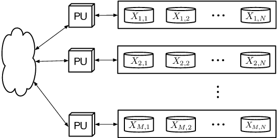
In this paper we introduce a realistic multi-rack storage network which represents the real data storage networks more generally and practically. We focus on a storage code-design framework, specifically tailored for multi-rack data storage networks and their requirements. Our storage network model depicted in Figure 2 consists of racks each of which contains storage nodes. We will assume that each rack has a Processing Unit (PU) which is directly connected to all storage nodes in the same rack. It is worth mentioning that in practical data centres all servers in a rack are connected to an in-rack switch which is called Top-of-Rack (ToR) switch. The ToR switch is responsible for the intra-rack communication while one or more servers in the rack could be used as compute nodes [22]. This architecture can be viewed as the Processing Unit of the rack. The rack processing unit is responsible for both computation on the stored data and communication between the nodes in the rack. Moreover, the processing units of racks can communicate to each other in order to transmit data from one rack to another (via aggregation switches [22]). In other words, storage nodes in two different racks can only communicate via their respective processing units. It is very common in realistic systems that the communication cost between the storage nodes within a rack (via its PU) is much lower than the communication cost between two different processing units (and hence located in two different racks) [8]. Therefore, it is desirable and in fact critical that a failed node could be repaired by only the survived nodes within the same rack in order to keep the repair cost low. We further assume that the system bottleneck is at the PU of each rack. Therefore, in our code-design framework, the focus is to design distributed storage codes that minimise the communication costs between nodes and the processing unit of the rack. It is only for some occasional severe failure patterns that it will require nodes from other racks to assist in the repair process.
Our multi-rack storage code is defined with three parity check matrices , , and . Matrix determines the intra-rack repair groups such that any failed node in any of the racks can be repaired by at most surviving nodes in the same rack. We derive the conditions on such that the intra-rack local repair can still be successful even in the presence of multiple failures in the rack. However, as mentioned earlier, in the case of severe failure patterns where the intra-rack repair fails, matrices and determine a group of helper nodes from the same rack of the failure and the other racks in order to proceed with the inter-rack repair. Moreover, in our coding scheme, parity matrix determines the group of helper racks during an inter-rack repair. We show that can be designed separately as the parity check matrix of a locally repairable code such that only a small group of racks participate in the inter-rack repair process.
In general, existing locally repairable coding schemes are not suitable candidates for practical multi-rack distributed storage networks. Assume that a repair group of an LRC is considered to be a rack. In the case that a local repair fails, the network will need other repair groups (racks) to help for the failure repair. This assumption is costly due to the geographically distributed nature of the storage networks. However, in our coding scheme, it is only in occasional sever failure patterns that the other racks are needed to help repairing the failure. Moreover, the existing LRC schemes do not take into account the different communication cost between the nodes. A major advantage of our coding scheme compared to similar schemes, such as LRCs, is the concept of the rack processing unit. In contrast to LRCs, our coding scheme enables the helper racks to only transmit a linear combination of the helper nodes’ content to the failed rack via their processing unit. This approach optimises the inter-rack repair bandwidth and significantly reduces the inter-rack communication cost.
I-A Related Work
A regenerating code [2] is proposed in [23] in order to minimise the across rack repair bandwidth. In this coding scheme, each rack stores multiple encoded symbols (rather than one symbol [11]) of a data block in distinct storage nodes. To repair a failed node, first a regeneration will be occurred within each rack (i.e., one of nodes in each rack collects the encoded data from all nodes in the rack and re-encodes it) and then the regenerated data from each rack will be transferred to the failed rack to regenerate the content of the failed node. Recently, heterogeneous distributed storage networks (including the multi-rack models) has received a fair amount of attention [24, 25, 26, 27, 28] due to the heterogeneous nature of the practical storage networks and their various applications such as hybrid storage systems [29], video-on-demand systems [30], and heterogeneous wireless networks [31]. A heterogeneous model for distributed storage networks is introduced in [28] where a static classification of the storage nodes is proposed. In this model the storage nodes are partitioned into two groups with ”cheap” and ”expensive” bandwidth. In other word, the data download cost, to repair a failure, from the nodes in the ”cheap bandwidth” group will be lower than the data download cost from the ”expensive bandwidth” group. The model in [28] partially addressed the issues that the communication costs among nodes are not all equal where the download cost from one of the groups is always cheaper than the other group. However, this model does not fit well into a multi-rack model, where the transmission cost should depend on both where the transmitting and the receiving (or the failed) storage nodes are located.
A more realistic rack model of a distributed storage network has been investigated in [25], in which the authors considered a two-rack model. In their model, the communication cost between the nodes in the same rack is smaller than between two different racks. Therefore, the main difference of this model compared to the one in [28] is that the classification of the storage nodes depends on the location of the failed node. More precisely, the data download cost from the nodes in the same rack (i.e., group) of the failure is lower (i.e., cheap bandwidth) than the download cost from the other group (i.e., expensive bandwidth). As such, it is desirable that more data should be transmitted by nodes in the same rack of the failed node during the repair process. Using an information flow graph, [25] derives the trade-off between the storage cost and repair cost by identifying that if certain choice of parameters are achievable or not. The trade-off in [28] and [25] is asymptotic (without restriction on the alphabet size) and functional repair is always assumed (i.e., the failed node is not required to recover exactly what it was previously storing, as long as the whole storage system is still robust after repair).
A non-homogenous storage system is considered in [27] where there exists a super node in the network with higher storage capacity, reliability and availability probability than the other nodes. It has been shown that this model can achieve the optimal bandwidth-storage trade-off bound in [2] with a smaller file and alphabet size than the traditional homogeneous storage network in [32].
The Data retrieval problem in heterogeneous storage systems is studied in [33]. In this model it is assumed that each node has a different storage size where any amount of encoded data can be stored in each node such that the total allocated storage remains less than a threshold. The optimal allocation to retrieve the original data is studied such that the data collector can access to only a random group of nodes. A combination of the repair problem with data allocation is investigated in [34] and [35]. In these works a general model of a heterogeneous storage network is considered where each node has a different storage and download cost. The amount of data allocated to each storage node and the amount of data to be downloaded from each survived node to repair a failure has been investigated using the information flow graph to minimise the storage and repair cost and establishing a storage-repair trade-off.
The capacity of heterogenous storage networks is studied in [36]. The proposed network in this work consists of storage nodes with different storage capacities and repair bandwidths. It is assumed that the repair bandwidth of each node depends on the repair group that the helper nodes belong to. The functional repair of node failures is assumed and the capacity of this network as the maximum amount of stored information in order to reach a level of reliability is studied.
Block Failure Resilient (BFR) codes are studied in [37]. The authors consider a distributed storage network with a single failure domain [38] where the storage nodes are divided in blocks (e.g. racks). The failure of a block will result in unavailability of the nodes in that block. Consider a storage network with nodes and blocks where each block contains nodes. BFR codes relax the node-repairability and data-reconstruction constraints of the regenerating codes such that any failed node within a block can be repaired by contacting any nodes of any available blocks (i.e., nodes in total). Moreover, the original data can be retrieved by contacting any nodes of any available blocks (i.e., nodes in total) where is the resilience parameter. For such a relaxation, similar to the regenerating codes, the storage per node and repair bandwidth trade-off is derived. Locally repairable BFR codes are also introduced in [37] such that a failed node can be repaired by contacting the nodes of a local group of blocks (e.g., cluster). One of the main differences of the network model in [37] with our model is that it is assumed that always during the repair process of a failed node, the other nodes of the same rack are also unavailable (i.e., single failure domain) and they are not able to contribute in the repair process. In our model, we assume that in non-severe failure patterns, the available nodes of the rack can locally repair the failed node.
A similar network model to our work is considered in [39] where the network consists of clusters (e.g., racks) each of them stores nodes. The network is fully connected such that the nodes within a cluster are connected via an intra-cluster link and the clusters are connected via an inter-cluster link. The proposed coding scheme is a generalisation of the regenerating codes [2] where a file of size symbols is encoded into symbols and stored across nodes in the network such that each node stores symbols. In order to repair a failed node, symbols will be downloaded each from any subset of clusters. These symbols are a function of the content (at most , symbols) of at most nodes in each helper cluster. Moreover, the content (at most , symbols) of local helper nodes will be downloaded to contribute in the repair process. Utilising the information flow graph under the functional repair settings, an upper bound on the file size is derived. For fixed values of , the bound gives the trade-off between storage and inter-cluster bandwidth. A lower bound on intra-cluster bandwidth is also obtained. Unlike our coding scheme where the inter-rack repair happens only in the case of severe failure patterns, a failed node in [39] always is repaired by the help of a group of clusters (racks). Note that, all the bounds obtained in the aforementioned papers [37, 39] are based on the information flow graph under functional repair settings.
The capacity of clustered storage systems is investigated in [40]. The proposed network model consists of storage node distributed over clusters each of which contains nodes each with storage size . A failed node is regenerated by downloading symbols each from nodes within the same rack and symbols each from nodes from each cluster. It is assumed that during the repair process, all other nodes are available and will be contacted (i.e., and ). Also , due to the lower inter-cluster communication bandwidth compared to the intra-cluster. Employing the information flow graph, the storage capacity of this network is obtained in terms of the node storage size , intra-cluster repair bandwidth , and inter-cluster repair bandwidth . Note that since the coding scheme is based on regenerating codes, in order to minimise the repair bandwidth all nodes need to help to repair the failure.
The availability of clustered storage networks is studied in [41]. The aim in this work is to partition storage nodes of the network into clusters of size (there could be an extra cluster of size ) such that any failed node in a cluster can be repaired by any of the remaining clusters (except the last cluster with less storage nodes) as its repair group. Then, the network is said to have availability . The objective is achieving high availability and low repair bandwidth. The storage per node vs repair bandwidth trade-off is characterised following the network information flow graph under the functional and exact repair settings. Some class of codes are also proposed to minimise the exact repair bandwidth.
The notion of codes with hierarchical locality has been studied in [42]. Codes with hierarchical locality are an extension on the codes with -locality which are introduced in [5] such that any code symbol can be recovered locally by at most other symbols even in the presence of an additional erasures. A -level hierarchical code is an linear code with locality parameters where depending on the number of the failures (i.e., ), there exists a punctured code with locality parameters that can repair the failures.
The fact that coding at large lengths allows better error-tolerance for a given overhead, motivated the work in [43]. One of the main challenges in the storage networks with large length codes is correlated failures which could happen due to e.g. a rack failure, a data centre failure, or failure of a power source shared by a group of servers (i.e., single failure domain [38]). This work views the code design for a distributed storage network as a two step process of 1)picking a topology and 2) optimising encoding/decoding efficiency and maximising reliability. The authors consider a simple grid-like topology (which is also extendable to the multi-rack storage networks) where each row and column of coded symbols has a bunch of parity equations and there are some global parity equations that depend on all symbols (i.e., tensor products of row and column codes, augmented with global parity equations). A lower bound on the field size of the Maximally Recoverable codes is obtained and the correctable erasure patterns by these codes are characterised. An asymptotically optimal family of Maximally Recoverable codes for one basic topology is also proposed.
Despite of the applications of the works in [42] and [43] in multi-rack storage networks, neither of them propose a general code design framework which is specifically tailored for multi-rack distributed storage network considering various network parameters such as different intra-rack and inter-rack communication cost. For example, assume that a storage code with hierarchical locality is employed in a multi-rack storage network. Depending on the failure pattern, it would need all the racks to be available to repair a failure which is not a practical assumption due to geographically distributed nature of the network. Moreover, in [42] and generally other LRC schemes in the literature, it is assumed that during a repair process, the content of each helper node will be transmitted separately to the failed node’s replacement (newcomer) in order to recover the lost data. In a multi-rack storage network, this will impose a high inter-rack repair bandwidth to the network due to the high inter-rack communication cost.
I-B Contributions and Organisation
The main contributions of this paper are:
- •
A code-design framework for multi-rack storage networks: we propose a general coding scheme for multi-rack distributed storage networks. Our proposed scheme is defined by three parity check matrices , , and . This coding scheme is able to locally repair any node failure within the rack by using matrix in order to minimise the repair cost. Moreover, in the case of severe failure patterns that the failures cannot be repaired only by the survived nodes inside the rack, by using matrix , our scheme is able to engage some of the nodes in other racks in the repair process. The helper racks will be determined by matrix .
- •
Establishing linear programming bounds on the code size: we show that maximising the rate of the multi-rack storage code is equivalent to maximising the code size. We establish a linear programming problem on the code size based on the definition and criteria of our multi-rack storage code. The maximum size of the code in turn will determine the optimal size of the parity check matrices and .
This paper is extended from our earlier work on multi-rack distributed storage codes [1] which is presented in IEEE Information Theory workshop (ITW 2014). The rest of this paper is organised as follows. In Section II we present the code-design framework for multi-rack storage networks and give a detailed description of its criteria and the failures repair processes. We also derive the code rate in this section. Then, In Section III, we establish a linear programming problem to upper bound the code size. Moreover, in this section, we exploit symmetry in our code in order to reduce the complexity of the problem. The paper is concluded in Section IV.
II Multi-rack Storage Code – Design Framework
In this section, we first introduce our system model and multi-rack storage code which is defined by three parity check matrices , , and . We then describe the intra-rack repair process and show how the failures can be repaired only by the surviving nodes inside the rack using the parity check matrix . The inter-rack repair process will be described afterwards where we show how a failure can be repaired by the surviving nodes inside the rack and the nodes in helper racks when the intra-rack repair fails. Finally, we present the rate of the multi-rack storage code which will be used in the next section to establish an upper bound on the code size.
Consider the rack model storage network depicted in Figure 2. This multi-rack data storage network consists of racks each of which contains storage nodes (or storage disks). We will represent each node as
where , , and is referred to the th node in the th rack. Abusing notations, will also be referred to the content stored at that particular storage node. We define
whose entries are from . Particularly, is the vector of encoded data stored in the rack . Collecting all the stored contents from each rack, we have
In this paper, we assume that each rack has a processing unit, which is responsible for all computations required in nodes repair. In other words, contents stored in a failed node will be regenerated in the processing unit, before sending all the regenerated content to the failed node (or its replica).
Definition 1 (Multi-rack storage codes).
A multi-rack storage code is defined by three parity check matrices over of respectively sizes , and . The three matrices induce a storage code such that must satisfy the following parity-check equations
| (4) | ||||
| (5) |
We will call respectively the intra-rack and inter-rack parity matrices. The matrix will be called helper-rack parity check matrix.
Later in Section III we will show that maximising the code rate is equivalent to maximising the size of the code which in turn can determine the optimal value of and . Moreover, we will show that the value of is only dependent on the network topology and can be chosen separately from and .
In multi-rack storage code, it is expected that most of the node failures should be recovered and repaired locally within their own racks. However, in the special case where local repair is not possible, redundancies added among rack will be used in the recovery. As there is a much lower probability that nodes in a rack cannot be recovered locally within the rack, this paper focuses on the special case where only one rack has node failures (or that all failed nodes in other racks can be completely repaired locally).
We now consider the first case where failures in a rack can be repaired by using only nodes within the rack.
II-A Intra-Rack Repair
In this subsection, we will describe how to repair nodes locally within a rack. Assume without loss of generality that rack 1 fails (i.e., a group of nodes fails inside the rack). Let be the index set for the nodes in rack 1 that fail. In other words, the values of (i.e., the node content) are unknown to the processing unit in rack 1. Let
where
In other words, is obtained from by replacing with for all .
Define as an diagonal matrix such that its entry is 1 if and is 0 otherwise. For simplicity, we will drop the subscript if it is understood from the context. Let be the complement set of . Therefore, will be the set of survived nodes in the rack . Consequently, . Recall that Therefore, rack 1 can repair ALL its failed nodes by the local rack survived nodes if and only if the following system of linear equations
| (6) |
has a unique solution. For notation simplicity, we will use to denote the vector space spanned by rows of and . The set of linear equations in (6) has a unique solution if and only if
| (7) |
Let be the smallest set such that . We will denote its size as . By definition, if , then it is sufficient to use intra-rack repair to repair all failed nodes.
Remark 1.
It is well known that is equal to the minimum distance of a linear code defined by the parity check matrix .
Definition 2 (support).
The support of a vector is a subset of such that if and only if , .
Definition 3.
Consider any matrix and vector (such that both have columns). For any , let
If is the zero vector, we will simply denote by .
Remark 2.
As we shall see, plays a fundamental role in determining whether failures in a rack can be repaired or not. Specifically, contains all intra-rack repair groups for . If there exists a set (or group) such that all are survived for all , then the failed node can be repaired by using only for all . The general case where is non-zero vector will be used in the inter-rack repair and will be explained soon.
Example 1.
Suppose is the intra-rack parity check matrix and is given by
| (8) |
From Definition 3, will be given by
where the entries are the index set of a group of nodes in each rack. Each subset in denotes a intra-rack repair group for repairing (or in general).
Lemma 1.
If , then there exist vectors , and such that
| (9) |
where is a length row vector such that
| (10) |
Conversely, if there exist vectors , and such that (9) holds, then there exists such that .
Proof.
Since , then there exists such that 1) for some vector and , 2) and 3) . Let . Since , . Hence,
The lemma thus follows by letting . The proof of the converse is straightforward and is omitted. ∎
Based on Lemma 1, the following theorem specifies conditions for intra-rack repair.
Theorem 1 (Intra-rack Repair).
Suppose node fails in rack . Let be the index set for all failed nodes11 1 can be interpreted as the set of failed nodes at the moment when the node is being repaired. (hence, ). If satisfies the following two criteria,
- 1.
, and
- 2.
,
then there exists for such that
| (11) |
Proof.
Equation (11) essentially defines how to regenerate the content of a failed node from for (i.e., the nodes in its repair group). In other words, node is a linear combination of the nodes in its repair group where the coefficients are . In this case, symbols are transmitted to the processing unit in rack 1, which can then repair the failed node by (11). Clearly, the choice of will affect the repair cost. It is always desirable to pick such that its size is as small as possible.
Example 2.
Let be the intra-rack parity check matrix over such that
Assume nodes and are failed. Thus, the failure pattern will be . Suppose we want to repair node . The repair groups of node is given by
A repair group is eligible for intra-rack repair process such that . Therefore, . Moreover, we choose . Then, and satisfying the conditions in Lemma 1. Therefore, the repair coefficients vector in (16) is given by
Consequently,
The remaining failure can also be repaired by the same procedure.
II-B Inter-Rack Repair
Communications across racks in a multi-rack storage network are in general more expensive. Consider the extreme case where each rack physically represents a data center, each of which is geographically distant from each other. In this case, data transmission across long distance is clearly more expensive than transmission within each rack. Therefore, it is often desirable to design codes such that more repairs can be done locally within racks. However, in some rare cases (e.g., burst failure within a rack), nodes failure cannot be repaired locally. For example, this may occur when node fails and for all , there is at least another node for which also fails. When intra-rack repair fails, inter-rack repair can be done. The idea is described below.
Let , and be respectively vectors spanned by the rows of the matrices , and . Then, it can be verified directly from (4) and (5) that
| (17) | ||||
| (18) |
where and is assumed to contain . Suppose and . Then
| (19) |
can be used to recover . Equation (19) consequently defines the across rack repairs. To be more precise, in order to repair the failed node , one would need 1) code symbols from the failing rack for , and 2) code symbols from rack for and . In other words, to repair a failed node a group of helper racks are identified by parity matrix . Also, a group of helper nodes in each helper rack is identified by parity matrix . The helper nodes in each helper rack will send their content to the rack process unit. Each helper rack process unit calculates a linear combination of the helper nodes content and send it to the process unit of the failed rack . The process unit of the failed rack calculates the sum of this information received from helper racks. A group of survived nodes from the failed rack which are specified by and send their content to the rack process unit. The process unit then calculates a linear combination of the information from these nodes and adds it to the information from the helper racks. This results in the information content of the failed node .
Theorem 2.
Suppose node fails in rack . Let be the index set for all failed nodes (hence, ). If satisfies the following criteria,
- 1.
- 2.
(i.e., )
- 3.
, and
- 4.
,
- 5.
then there exists for and for such that
| (20) |
Remark 3.
The interpretation of the theorem is as follows: The support of corresponds to index of nodes in the “helper racks”. Clearly, the smaller is the support the better, in order to minimise transmission cost. However, we would also point out that the transmission costs required to transmit across racks does not depend on the support size of . More precisely, for each helper rack, only the sum is required to be transmitted, instead of specific individual . On the other hand, the set denotes the set of nodes which can be used to repair . Consequently, and (index set for the failed nodes in rack ) must be disjoint. Finally, is the index set of the helper racks. Note also that Theorem 2 reduces to Theorem 1 if and is the zero vector.
Remark 4.
As a consequence of Theorem 2, The processing unit in rack where , will retrieve symbols. The processing unit of rack 1, will need to retrieve symbols within the rack. Also, one symbol transmission is needed for the processing unit of rack 1 to send the recovered symbol back to the failed storage node . Finally, each helper rack indexed in will transmit 1 symbol to the processing unit of rack 1. Summing up all these transmissions, there are in total 1) symbol transmission within racks, and 2) symbol transmissions across racks.
Example 3.
Consider a rack model storage network with racks, each of which contains storage nodes. Suppose the parity check matrices are as follows:
and
Note that the code is over . Suppose node fails. Then by Definition 3, it can be verified that
In particular, any subset of nodes in rack indexed by can be used to repair .
Now, suppose that the following nodes failed in rack 1 (i.e., ). In this case, cannot be repaired via intra-rack repair since there exist no intra-rack repair group such that . Therefore, inter-rack repair is needed. Let and hence following from criterion 1 and 2, respectively. Moreover, let and following from criteria 3–5, respectively. Note that, , , and indicate the group of helper racks, the group of helper nodes in the helper racks, and a repair group in rack 1 which will participate in repairing the failed node .
Choose , , , , and such that
| (21) | ||||
| (22) |
are satisfied where (21) and (22) follow from Lemma 1, and is defined in (61). Following from (59) and (A), we have
and
Now, the failed node can be recovered by (20) such that
In this example a total number of 18 symbol transmissions within the racks and 3 symbol transmissions across the racks are needed to repair the failed node .
When we need to repair multiple failed nodes (say of them) via inter-rack repair, the cost is not simply times: First, it is possible that a transmission from inter-rack can be used to repair for more than one node. Second, once inter-rack repair has been achieved, nodes which are previously not repairable via intra-rack repair may become repairable. To be more precise, suppose nodes fail where . In this case, nodes failure may not be able to be recovered merely via intra-rack repairs. Let be of size . In that case, in the worst case scenario, one can at least aim to recover variables for via inter-rack repair first. Once this is achieved, the remain nodes can be recovered via intra-rack repair. Following the idea, the following theorem gives an upper bound on the repair transmission cost.
Theorem 3 (Upper bound on transmission costs).
Let be the index set of all failed nodes in rack . Suppose that 1) for any , there exists satisfying the criteria in Theorem 6 where and 2) for any , there exists satisfying the criteria in Theorem 1 where . Then the required total transmissions within a rack and across racks are respectively upper bounded by
| (23) | ||||
| (24) |
II-C Code Rate
In this subsection we derive the rate of our proposed code for multi-rack storage networks. The code rate will later be employed to establish the upper bound of the code size in Section III. The following theorem gives the rate of the multi-rack storage code.
Theorem 4.
Let , , and be respectively , , and matrices. Then the rate of the multi-rack storage code is lower bounded by
| (25) |
Equality holds if rows in and are linearly independent, and is a full rank matrix.
III Bounds
In this section, we first derive the relations between the code rate, code size, and the size of the parity check matrices. We show that under some constraints, maximising the code rate is equivalent to maximising the size of the code which in turn can determine the optimum size of the parity check matrices. We define the multi-rack storage network parameters such as intra- and inter-rack resilience and locality in order to establish a Linear Programming (LP) problem to maximise the size of the multi-rack storage code. Then, the symmetries in the problem will be used to significantly reduce the complexity of the LP problem.
III-A Linear Programming Bound
In the previous section, we introduced a class of storage codes called multi-rack storage codes and explained how to repair nodes failure via intra-rack or inter-rack repairs. In this section, we will develop bounds for this class of codes. Recall our code construction and definition. We will notice the following:
- 1.
The intra-rack parity check matrix or more precisely the support of the dual codewords spanned by the rows of determines how failed nodes can be repaired locally within a rack. Alternatively, the dual codewords spanned by intra-rack parity check matrix and inter-rack parity check matrix together defines the inter-rack repair process.
- 2.
The helper-rack parity check matrix specifies which racks can be used in the inter-rack repair process. Naturally, one would prefer to involve only a small number of racks to minimize the inter-rack transmission cost.
Assuming without loss of generality that all rows of and are independent and that is full rank, Theorem 4 shows that
| (26) |
or equivalently,
| (27) |
The rate of the multi-rack storage code is essentially determined by the size of the matrices and .
Understanding their roles, we can immediately recognise that one can separately design and . The design of will affect the number of helper racks needed in inter-rack repair. In fact, it is very similar to the design of locally repairable codes. The idea is to design a linear code (specified by the parity check matrix ) such that for any , there are dual codewords with a small support containing . If the racks are geographically separated and connected to a network, the design of may take into account the network topology and the costs of the transmission links. For example, an algorithm for the design of linear binary locally repairable codes over a network can be found in [16]. There are also previous works including our own work in [19] and [18] which discuss the design and bounds for locally repairable codes. On the other hand, the design of and will affect the code’s ability in intra-rack and inter-rack repair. The focus of the remaining paper is on understanding the fundamental limits of the best design of these two matrices.
Separating the design of from , we can simply consider a simple special case where there are only two racks (i.e., ) and that
Assume without loss of generality, we may characterise our multi-rack storage code via the following parity-check equations:
| (28) | ||||
| (29) | ||||
| (30) |
As such, we will simply refer a multi-rack storage code as .
Definition 4.
We call a multi-rack storage code as a linear multi-rack storage code if it satisfies the following conditions:
- 1.
(Intra-rack resilience) Any node failures in a rack can be repaired via intra-rack repair;
- 2.
(Intra-rack locality) For any node failure pattern in a rack, each node can be repaired via intra-rack repair, involving at most surviving nodes;
- 3.
(Inter-rack resilience) Any node failures in a rack can be repaired via inter-rack repair.
- 4.
(Inter-rack locality) For any node failure pattern in a rack, each node can be repaired via inter-rack repair such that involving ) at most surviving nodes in the failing rack and ) at most nodes from each helper rack.
The definition for linear multi-rack storage code can be made more precise via the use of support enumerators, to be described as follows.
To simplify our notation, we may use and instead of and . Let
| (31) |
We call the codebook. Clearly, the design of and the design of are equivalent.
Definition 5 (Support).
Consider any codeword where and . Its ”support” is a tuple such that and , where
| (32) | |||
| (33) |
for all . For notation simplicity, we will simply denote that
Remark 5.
Definition 6 (Support enumerator).
The enumerator function of the code is defined as
| (34) |
for all .
The below theorem gives properties of a multi-rack storage code. As we shall see, these properties will form constraints in our linear programming bound.
Theorem 5.
For any multi-rack storage code , the support enumerators of and its dual satisfy the following properties:
- 1.
Dual codeword support enumerator:
(35) where
- 2.
Symmetry: For all ,
(36) - 3.
Intra-rack resilience: For all such that
(37) - 4.
Intra-rack locality: For any ,
(38) where
- 5.
Inter-rack resilience: For all such that
(39) - 6.
Inter-rack locality: For any ,
(40) where
Lemma 2.
Consider a multi-rack storage code . Suppose the dimensions of the matrices are respectively , , and . Then
| (41) |
and
| (42) |
Hence, the rate of the code is
| (43) |
Proof.
First, it is clear that is equal to the size of the following set
As the dimensions of and are respectively , and , the size of the set is obviously leading to (41)
Remark 6.
According to (43), the rate of the storage code is clearly nonlinear, with respect to the support enumerator . However, if we fix
then maximising is equivalent to maximising .
Theorem 6 (Upper bound).
Consider fixed , and and a multi-rack storage code such that
Let be the maximum of the following linear programming problem.
Linear Programming Problem (LP1)
| subject to | ||||
| (C1) | ||||
| (C2) | ||||
| (C3) | ||||
| (C4) | ||||
| (C5) | ||||
| (C6) | ||||
| (C7) | ||||
| (C8) | ||||
| (C9) | ||||
| (C10) |
Then is upper bound by
Proof of Theorem 6.
We define
As mentioned earlier, maximizing the code rate is equivalent to maximize the code size which is the objective function of the linear programming problem LP1. The first constraint of the optimization problem LP1 follows from the fact that the number of codewords are non-negative. The second constraint follows from the symmetry property of the code. The constraint (C3) follows from the dual code support enumerator property (MacWilliam’s identity) in Theorem 5. Constraint (C4) follows from the fact that the number of dual codewords are non-negative. Constriant (C5) follows from the fact that there exists only one zero codeword in code . Constraints (C6)–(C9) follow from the properties 3–6 in Theorem 5. ∎
Remark 7.
Strictly speaking, to optimise , one also needs to optimise the choice of , which is generally unknown. However, as . Hence, we have
where is the maximum of (LP1) when .
III-B Bound Simplification via Symmetry
The complexity (in terms of the number of variables and the number of constraints) of the linear programming problem LP1 in Theorem 6 will increase exponentially with the number of storage nodes in each rack. However, if we notice the LP1 carefully, we can observe that the problem itself has much symmetries in it such that exploiting this inherent symmetry can significantly reduce the problem complexity.
Let be the symmetric group on , whose elements are all the permutations of the elements in which are treated as bijective functions from the set of symbols to itself. Clearly, . The variables in the optimization problem LP1 are
Let be a permutation on such that . For each , we extend the mapping by defining
Due to the symmetries, we have the following proposition.
Proposition 1.
Suppose satisfies all the constraints in the linear programming problem LP1 in Theorem 6. For any , let
| (44) | ||||
| (45) |
Then also satisfies the constraints in LP1, with the same values in the objective function. In other words,
Proof.
The proposition follows directly from the symmetry in the constraint and optimising function. ∎
As the feasible region in the linear programming problem (LP1) is convex, we have the following corollary.
Corollary 1.
Let
| (46) | ||||
| (47) |
Then also satisfies the constraints in (LP1) and
| (48) |
Proof.
By Corollary 1, it is sufficient to consider only ”symmetric” feasible solutions of the form in LP1. In other words, one can impose additional symmetric constraint to LP1 without affecting the value of the objective function.
One important benefit for considering is that many terms in the linear programming bound can become alike (and hence can be grouped together).
Proposition 2 (Grouping alike terms).
Suppose such that
| (49) | ||||
| (50) | ||||
| (51) |
Then and .
Due to Proposition 2, we can impose the following additional constraint on (LP1)
| (52) | ||||
| (53) |
for all satisfying (49) - (51). As many of these variables are now the same, one can greatly reduce the number of variables in (LP1).
Theorem 7 (Simplified LP Bound).
The maximum in (LP1) is the same as the maximum of the following linear programming problem:
Remark 8.
In (LP1), the number of variables and constraints grows exponentially with – the number of nodes in a rack. Such exponential growth makes (LP1) practically infeasible to solve for moderate . However, via reduction by symmetry, the number of variables in (LP2) has greatly reduced to while the number of constraints to Clearly, the reduction is significant.
Example 4.
We consider a very simple setup to show how some of the constraints in linear programming bound in (LP2) are calculated. Let, is the number of the storage nodes in each rack. As mentioned earlier in Section III-A parity matrix can be design separately, hence the number of the racks will not affect the LP bound. Moreover, let , , , , , , and . Then, we have and . Here, we show how to calculate , , and . Following (90) and (93), respectively,
In order to calculate from (106), we need to find all possible values of for each fixed tuples of and all tuples of such that , , , , , . Then , , and can be calculated from (100), (101), and (105), respectively. For instance, let . Then for a tuple , one possible combinations for will be . Therefore,
Another possible combination will be . Therefore,
As mentioned earlier, all values of must be calculated (this can be done by a computer simulation code e.g. in MATLAB) for all and in order to calculate . Figure 3 illustrates of selecting the different combinations for . The numbers in red and green are the two aforementioned different possible combinations for . The combinations will be chosen such that the sum of the rows and columns satisfy the values of and .

IV Conclusion
In this paper we introduced a code-design framework for multi-rack distributed data storage networks. In this model the encoded data is stored in storage nodes distributed over multiple racks. Each rack has a process unit which is responsible for all calculations and transmissions inside the rack. Practically, the cost of data transmission within a rack is much less than the data transmission across the racks. Therefore, it will be a significant reduction in the repair bandwidth if the node failures are repaired locally inside the racks. Our multi-rack distributed storage code is defined with three parity check matrices , , and . We proposed a code-design framework for multi-rack storage networks which is able to locally repair the node failures within the rack using the parity check matrix in order to minimise the repair cost. However, under the severe failure circumstances where the failures are not repairable by only the survived nodes inside the rack, our coding scheme is capable of engaging the storage nodes in other racks in helping the surviving nodes inside the failed rack to repair the failures where the parity check matrices and determine the helper racks and the helper nodes, respectively. We justify that the parity matrix can be designed separately from the matrices and where indeed it can be designed as the parity check matrix of a locally repairable code such that only a small group of racks need to participate in an inter-rack repair. We established the relation between the rate and the size of the multi-rack storage code and showed that maximising the rate of our multi-rack storage code is equivalent to maximising the code size. In order to maximise the code size, we established a linear programming problem based on the code-design framework criteria. These bounds characterise the trade-off between different code parameters such as inter- and intra-rack resilience and locality. We also exploited symmetries in the linear programming problem for simplifying and significant reductions in its complexity.
References
- [1] M. A. Tebbi, T. H. Chan, and C. Sung, “A code design framework for multi-rack distributed storage,” in proc. Information Theory Workshop (ITW), 2014 IEEE, Nov. 2014, pp. 55–59.
- [2] A. G. Dimakis, P. B. Godfrey, Y. Wu, M. J. Wainwright, and K. Ramchandran, “Network coding for distributed storage systems,” IEEE Trans. Inf. Theory, vol. 56, no. 9, pp. 4539–4551, Sep 2010.
- [3] N. B. Nihar, K. V. Rashmi, P. V. Kumar, and K. Ramchandran, “Distributed storage codes with repair-by-transfer and nonachievability of interior points on the storage-bandwidth tradeoff,” IEEE Trans. Inf. Theory, vol. 58, no. 3, pp. 1837–1852, Mar. 2012.
- [4] C. Suh and K. Ramchandran, “Exact-repair mds code construction using interference alignment,” IEEE Trans. Inf. Theory, vol. 57, no. 3, pp. 1425–1442, Mar. 2011.
- [5] G. M. Kamath, N. Prakash, V. Lalitha, and P. V. Kumar, “Codes with local regeneration and erasure correction,” IEEE Trans. Inf. Theory, vol. 60, no. 8, pp. 4637–4660, August 2014.
- [6] D. S. Papailiopoulos and A. G. Dimakis, “Locally repairable codes,” in proc. IEEE Int. Symp. Information Theory, Cambridge, MA, July 2012, pp. 2771–2775.
- [7] T. C. Jepsen, Distributed Storage Networks: Architecture, Protocols and Management. John Wiley, 2003.
- [8] G. Ananthanarayanan, S. S. A. Ghodsi, and I. Stoica, “Disk-locality in datacenter computing considered irrelevant,” in USENIX HotOS, 2011.
- [9] F. Ahmad, S. T. Chakradhar, A. Raghunathan, and T. N. Vijaykumar, “Shufflewatcher: Shuffle-aware scheduling in multi-tenant mapreduce clusters,” in Proc. USENIX ATC ’14: 2014 USENIX Annual Tchnical Conference, Philadelphia, PA, June 2014.
- [10] C. Huang, H. Simitci, Y. Xu, A. Ogus, B. Calder, P. G. J. Li, and S. Yekhanin, “Erasure coding in windows azure storage,” in Proc. of USENIX ACT, 2012.
- [11] M. Sathiamoorthy, M. Asteris, D. Papailiopoulos, A. G. Dimakis, R. Vadali, S. Chen, and Borthakur, “Xoring elephants: Novel erasure codes for big data,” in Proc. of VLDB Endowment, 2013.
- [12] T. Benson, A. Akella, and D. A. Maltz, “Network traffic characteristics of data centers in the wild,” in Proc. of ACM IMC, 2010.
- [13] D. Papailiopoulos, J. Luo, A. Dimakis, C. Huang, and J. Li, “Simple regenerating codes: Network coding for cloud storage,” in proc. IEEE INFOCOM, March 2012, pp. 2801–2805.
- [14] K. V. Rashmi, N. B. Shah, P. V. Kumar, and K. Ramchandran, “Explicit construction of optimal exact regenerating codes for distributed storage,” in proc. IEEE 47th Annu. Allerton Conf. Commun., Control, Comput., Urbana, IL, Sep 2009, pp. 1243–1249.
- [15] P. Gopalan, C. Huang, H. Simitci, and S. Yekhanin, “On the locality of codeword symbols,” IEEE Trans. Inf. Theory, vol. 58, no. 11, pp. 6925–6934, Nov. 2012.
- [16] Q. Yu, C. W. Sung, and T. H. Chan, “Locally repairable codes over a network,” in proc. Information Theory Workshop (ITW). IEEE, Nov. 2014, pp. 70–74.
- [17] L. Pamies-Juarez, H. D. Hollmann, and F. Oggier, “Locally repairable codes with multiple repair alternatives,” in proc. IEEE Int. Symp. Information Theory, 2013, pp. 892–896.
- [18] M. A. Tebbi, T. H. Chan, and C. Sung, “Linear programming bounds for robust locally repairable storage codes,” in proc. Information Theory Workshop (ITW), 2014 IEEE, Nov. 2014, pp. 50–54.
- [19] T. H. Chan, M. A. Tebbi, and C. W. Sung, “Linear programming bounds for storage codes,” in 9th International Conference on Information, Communication, and Signal Processing (ICICS 2013), Dec. 2013.
- [20] A. S. Rawat, A. Mazumdar, and S. Vishwanath, “On cooperative local repair in distributed storage,” in 48th Annual Conference on Information Sciences and Systems (CISS), March 2014, pp. 1–5.
- [21] C. Huang, M. Chen, and J. Li, “Pyramid codes: Flexible schemes to trade space for access efficiency in reliable data storage systems,” Microsoft Research, Tech. Rep. MSR-TR-2007-25, March 2007.
- [22] Cisco Validated Design I, “Cisco data center infrastructure 2.5 design guide,” Cisco Systems, Inc., San Jose, CA, USA, Dec. 2007.
- [23] Y. Hu, P. P. C. Lee, and X. Zhang, “Double regenerating codes for hierarchical data centers,” in proc. IEEE Int. Symp. Information Theory, Barcelona, Spain, July 2016.
- [24] B. Gaston, J. Pujol, and M. Villanueva, “A realistic distributed storage system: the rack model.” [Online]. Available: arXiv:1302.5657v1
- [25] ——, “A realistic distributed storage system that minimizes data storage and repair bandwidth,” in Data Compression Conference (DCC), 2013, March 2013, pp. 491–491.
- [26] J. Pernas, C. Yuen, B. Gaston, and J. Pujol, “Non-homogeneous two-rack model for distributed storage systems,” in proc. IEEE Int. Symp. Information Theory, Istanbul, Turkey, Dec. 2013, pp. 1237–1241.
- [27] V. T. Van, C. Yuen, and J. Li, “Non-homogeneous distributed storage systems,” in proc. IEEE 50th Annu. Allerton Conf. Commun., Control, Comput., Allerton House, UIUC, Illinois, USA, October 2012, pp. 1133–1140.
- [28] S. Akhlaghi, A. Kiani, and M. R. Ghanavati, “Cost-bandwidth tradeoff in distributed storage systems,” Computer Communications, vol. 33, no. 17, pp. 2105–2115, Nov. 2010.
- [29] J. Kubiatowicz, D. Bindel, Y. Chen, S. Czerwinski, P. Eaton, D. Geels, R. Gummadi, S. Rhea, H. Weatherspoon, W. Weimer, C. Wells, and B. Zhao, “Oceanstore: An architecture for global-scale persistent storage,” in Proc. 9th Int. Conf. Architectural Support Programm. Lang. Oper. Syst., Boston, MA, Nov. 2000, pp. 190–201.
- [30] H. Zhang, M. Chen, A. Parek, and K. Ramchandran, “A distributed multichannel demand-adaptive p2p vod system with optimized caching and neighbor-selection,” in Proc. of SPIE, San Diego, CA, 2011.
- [31] N. Golrezaei, A. G. Dimakis, and A. F. Molisch, “Wireless device-to-device communications with distributed caching,” in proc. IEEE Int. Symp. Information Theory, 2012.
- [32] D. S. Papailiopoulos, A. Dimakis, and V. Cadambe, “Repair optimal erasure codes through hadamard designs,” in proc. IEEE 49th Annu. Allerton Conf. Commun., Control, Comput., Sep. 2011, pp. 1382–1389.
- [33] D. Leong, A. G. Dimakis, and T. Ho, “Distributed storage allocations,” IEEE Trans. Inf. Theory, vol. 58, no. 7, pp. 4733–4752, 2012.
- [34] Q. Yu, K. W. Shum, and C. W. Sung, “Minimization of storage cost in distributed storage systems with repair consideration,” in Proceedings of IEEE Global Communications Conference (GLOBECOM’11), Houston, Texas, Dec. 2011, pp. 1–5.
- [35] ——, “Tradeoff between storage cost and repair cost in heterogeneous distributed storage systems,” Trans. Emerging Tel. Tech, no. 26, pp. 1201–1211, 2015.
- [36] T. Ernvall, S. E. Rouayheb, C. Hollanti, and H. V. Poor, “Capacity and security of heterogeneous distributed storage systems,” IEEE Journal on Selected Areas In Communications, vol. 31, no. 12, pp. 2701–2709, Dec. 2013.
- [37] G. Calis and O. O. Koyluoglu, “Architecture-aware coding for distributed storage: Repairable block failure resilient codes,” Feb. 2017. [Online]. Available: arXiv:1605.04989v2
- [38] D. Ford, F. Labelle, F. I. Popovici, M. Stokely, V. A. Truong, L. Barroso, C. Grimes, and S. Quinlan, “Availability in globaly distributed storage systems,” in Proc. 9th USENIX Symposium on Operating Systems Design and Implementation, Vancouver, BC, CA, Oct. 2010.
- [39] N. Prakash, V. Abdrashitov, and M. Medard, “The storage versus repair-bandwidth trade-off for clustered storage systems,” IEEE Trans. Inf. Theory, vol. 64, no. 8, pp. 5783–5805, Aug. 2018.
- [40] J. yong Sohn, B. Choi, S. W. Yoon, and J. Moon, “Capacity of clustered distributed storage,” in 2017 IEEE International Conference on Communications (ICC), Paris, France, May 2017.
- [41] S. Sahraei and M. Gastpar, “Increasing availability in distributed storage systems via clustering,” in Proc. IEEE International Symposium on Information Theory (ISIT), Vail, Colorado, USA, June 2018, pp. 1705–1709.
- [42] B. Sasidharan, G. K. Agarwal, and P. V. Kumar, “Codes with hierarchical locality,” in Proc. IEEE International Symposium on Information Theory (ISIT), June 2015.
- [43] P. Gopalan, G. Hu, S. Kopparty, S. Saraf, C. Wang, and S. Yekhanin, “Maximally recoverable codes for grid-like topologies,” in Proc. Twenty-Eighth Annual ACM-SIAM Symposium on Discrete Algorithms (SODA ’17), Barcelona, Spain, Jan. 2017, pp. 2092–2108.
- [44] F. J. Macwilliams and N. J. A. Sloane, The Theory of Error Correcting Codes, North Holland, Amsterdam, 1977.
Appendix A Proof of Theorem 2
By Criterion 1), there exists a row vector of length such that
| (54) |
In other words, is a vector from row space of . From Lemma 1, as by Criterion 3, there exist row vectors , and such that
| (55) |
Now, notice
| (56) | ||||
| (57) | ||||
| (58) |
where the last equality follows from (4). Let
| (59) |
Then
Consequently,
| (60) |
Let , be a length row vector such that
| (61) |
Then
and hence
| (62) | ||||
| (63) |
From Lemma 1, since , there exist vectors and such that
| (64) |
Now, notice that is a matrix over , as has only columns. Consequently,
| (65) | ||||
| (66) |
where the last equality follows from that
| (67) | ||||
| (68) | ||||
| (69) |
where the last equality follows from (5).
Let the matrix
| (73) |
as is a diagonal matrix. If and , then it can be verified easily that
- 1.
and hence if either or .
- 2.
(74)
Thus the theorem is then proved.
Appendix B Proof of Theorem 3
First, we will consider intra-rack transmissions. In each helper rack (say ) involved in the inter-rack repair, nodes in it will need to transmit its data ( where ) to the processing unit in the helper rack. So, the set of symbols sent from the nodes to the processing unit is . Consequently, the total number of symbols sent to the processing units of helper rack is equal to where is the number of helper racks. That explains the first term in LHS of (23). Next, at each helper rack , it will need to transmit
to the failing rack. As these symbols may be linearly dependent, the actual number of symbols that really needed to be transmitted is only . Therefore, the total number of inter-rack transmission is . This explains the upper bound on (24).
After receiving the transmissions from the helper racks, the processing unit of the failed rack can now aim to recover the failed nodes. For each , it requires transmission from nodes in the set . Therefore, the number of intra-rack transmissions in rack 1 from nodes to the processing unit is . This corresponds to the second term in RHS of (23). Finally, receiving all the symbols, the processing nodes can recover the contents of all the failed nodes. It requires intra-rack transmissions from the processing unit of the failed rack to the failed nodes for recovery, explaining the last term of LHS of (23). The theorem thus proved.
Appendix C Proof of Theorem 4
According to (4) and (5), the total number of parity check equations is at most while the number of variables is . Therefore, the rate of the code is at least
Now, Consider the following set
In other words, is the set of solutions for the system of linear equations specified by parity check matrices and in (4) and (5), respectively. From linear algebra, the number of these solutions for any is given by
where is the field size. Similarly, let
| (75) |
where . Then for any .
Now, consider the set
Then it is clear that
where
As the rank of is and is a matrix of size , . Consequently,
| (76) | ||||
| (77) |
The theorem then follows.
Appendix D Proof of Proposition 2
By definitions,
| (78) | ||||
| (79) |
Now, by (49)–(51), there exists a permutation such that and . Hence, for any permutation , we have
| (80) |
Similarly, we have . Consequently,
| (81) | ||||
| (82) | ||||
| (83) | ||||
| (84) | ||||
| (85) |
where the second last equality follows from the fact that is a group and hence
Similarly, we can also prove that .
Appendix E Proof of Theorem 5
Recalling our assumptions in Section III, any codeword from the rack model storage code is in the form of satisfying (31). The support enumerator of the dual code in (35) follows from the MacWilliam’s identity [44]. Equation (36) follows directly from definition in (31). From the intra-rack resilience property in Definition 4, any simultaneous failures in a rack can be repaired via intra-rack repairs. Now consider such that . Suppose to the contrary that (37) does not hold, i.e., for some . Assume without loss of generality that . Then there exists a codeword such that
- 1.
and hence
- 2.
for all
Hence, if the nodes fail, then it is impossible to perfectly recover for all since the failing rack cannot distinguish whether the stored symbol was or . Therefore, we prove (37).
Follows from the inter-rack resilience property in Definition 4, any simultaneous failures in one rack can be recovered by the survived nodes in the same rack and all the nodes in the other rack. Again, suppose to the contrary that for some such that . Assume without loss of generality that . Then there exists a codeword such that
- 1.
and hence
- 2.
for all
Hence, if nodes fail, then it is impossible to perfectly recover for all . Thus, we prove (39).
From the intra-rack locality property, if the number of failures in a rack is at most , then each node can be repaired via intra-rack repair, involving at most surviving nodes. Now, suppose that the set of failing nodes is where . In order to repair the failed nodes via intra-rack repair, there must exists a dual codeword whose support is for some . Hence,
| (86) |
In fact, since supports of and are the same for all non-zero , we have
| (87) |
and (38) is proved.
Finally, from the inter-rack locality property, if the number of failures in a rack is at most , then each node can be repaired via inter-rack repair such that involving ) at most surviving nodes in the failing rack and ) at most nodes from each helper rack. Now, suppose that the set of failing nodes is where . In order to repair the failed nodes via intra-rack repair, there must exists a dual codeword whose support is . Again, as support of and for all non-zero , (40) thus follows.
Appendix F Proof of Theorem 7
The simplified bound is obtained by respectively replacing and with newly introduced variables and where
| (88) |
The replacement is possible, due to Proposition 2.
With the new notations, some terms will become alike and can be grouped together. For example, the term can be replaced by . Moreover, some constraints will become equivalent and hence can be omitted. Most constraints in (LP1) can be rewritten directly. The more complicated ones are (C3), (C8) and (C9). In the following, we will illustrate how to simplify and rewrite them.
We now first “reduce” constraint (C8). The key idea of reduction is described as follows: First, by Proposition 2, if . In fact, by (88),
Consider any given . Recall that
| (89) |
Let . By direct counting, we can prove that
| (90) |
Note that is independent of the choice of and . Then, the collection of constraint (C8) is reduced to one single constraint
| (91) |
The reduction of constraint (C9) is very similar to that of (C8). Again, consider any given . Recall that
Let
where . Hence, the constraint (C9) can be rewritten as
| (92) |
where .
Finally, it remains to determine . Partition into two sets
and
Hence,
| (93) |
where, by direct counting,
| (94) | |||
| (95) |
Finally, we will consider the reduction of (C3). The approach is similar, despite that the derivation is much more tedious. First, we fix a given . Consider the term
in (C3). Let
| (96) | ||||
| (97) | ||||
| (98) | ||||
| (99) |
and
Suppose for all Let . Then
- 1.
where
(100) Similarly, where
(101) - 2.
.
- 3.
where
(102) (103) (104) - 4.
Fix . Let Then
(105) - 5.
For any , let
(106) where
Grouping all the like terms, the constraint (C3) can be rewritten as in (D3).