Density estimates for degenerate double-well potentials

Phase coexistence models study the separation interfaces between regions corresponding to different values of a suitable state parameter. A typical model, introduced by J. D. van der Waals [MR523642] and developed, under various perspectives, by S. M. Allen, J. W. Cahn and J. E. Hilliard [CH, AC], and (in the vectorial setting) by V. L. Ginzburg, L. D. Landau and L. P. Pitaevskiĭ [MR0105929, MR0237287], considers a domain $\Omega\subseteq\mathbb{R}^{n}$ and a state parameter $u:\Omega\to[-1,1]$. In such model, the “pure phases” correspond to the values of the state parameters $1$ and $-1$ and the phase separation is driven by the minimization of an energy functional.

The typical energy functional taken into account is the superposition of a potential energy induced by a “double-well” function $W$, which tries to force the system into the pure phases, and an interaction energy (e.g. a gradient penalization) which avoids the production of unnecessary interfaces. More precisely, the potential energy is often taken of the form

with $W\geqslant 0$ and $W(\tau)>0=W(-1)=W(1)$ for any $\tau\in(-1,1)$, and a natural candidate for the interaction energy is the Dirichlet form

In this setting, the total energy becomes

and the critical points are solutions of

Probably, the most commonly studied case is that in which $W(\tau)=\frac{|1-\tau^{2}|^{2}}{4}$: in this case, formula (1.2) reduces to the so-called Allen-Cahn equation

A natural problem in phase separation models is then to “describe the picture seen from afar”: namely, one can expect that, at a large scale, the two phases tend to “separate” one from the other, with “the least possible interface”.

Till now, two main approaches have been adopted to rigorously describe this phase separation. The first method relies on the theory of $\Gamma$-convergence, and aims at identifying a limit functional and preserving the notion of minimizers. The second method is based on density estimates, that is on measuring which portion of the domain the two phases occupy, and gives as a byproduct the convergence of the level sets in the Hausdorff distance.

Very roughly speaking, both the methods of $\Gamma$-convergence and density estimates consider the scaled problem obtained by a spatial dilation of a minimizer. Namely, if $u$ is a minimizer of the energy functional and $\varepsilon\in(0,1)$ is a small parameter, one considers

One of the results of the $\Gamma$-convergence theory, as established in [MR0445362] and greatly extended in [MR1036589, MR1097327], is that, as $\varepsilon\searrow 0$, the function $u_{\varepsilon}$ converges (up to a subsequence) in $L^{1}_{\rm loc}(\mathbb{R}^{n})$ to a function $u_{0}$ which takes values only in $1$ and $-1$ (i.e. the state parameters of $u_{0}$ are only pure phases); remarkably, if one defines $E:=\{u_{0}=1\}$, then $\partial E$ is a minimal surface, namely $E$ is a local minimizer of the perimeter functional. In addition, a suitable rescaling of the original energy functional possesses appropriate convergence properties to the perimeter functional, and this convergence is compatible with energy minimization (see also [MR1968440] for a general introduction to this topic).

The second approach, based on density estimates, has been introduced in [CC], and several extensions also to inhomogeneous, singular and degenerate equations were performed in [MR2099113, MR2126143, MR2139200]. A general approach to density estimates was also presented in [FV], and the vector-valued case has been treated in [MR3393249]. See also the recent monograph [ALI] for more exhaustive discussions on density estimates for phase transitions.

The basic idea of the density estimates is to consider a point, say the origin, which belongs to the interface, say for concreteness $u(0)=0$, and measure the proportion of the sets $\{u>1/2\}$ and $\{u<-1/2\}$ in a large ball. In this configuration, one aims at showing that the Lebesgue measure of $B_{r}\cap\{u\in[-1/2,1/2]\}$ is bounded from above by $O(r^{n-1})$, while the Lebesgue measures of $B_{r}\cap\{u>1/2\}$ and $B_{r}\cap\{u<-1/2\}$ are bounded from below by $O(r^{n})$ for large $r$. That is, state parameters close to the pure phases occupy a considerable portion of the space on a large scale, while the interface becomes relatively negligible in measure.

A consequence of these density estimates is also that the level sets of $u_{\varepsilon}$ converge locally in the Hausdorff distance to $\partial E$: more precisely, for any $\delta$, $R>0$, there exists $\varepsilon_{0}(\delta,R)$ such that if $\varepsilon\in\big(0,\,\varepsilon_{0}(\delta,R)\big)$ then

It is clear that the $\Gamma$-convergence and the density estimates approaches share a common interest in the large-scale phase separation regimes, but address this problem with different methods and obtaining different results. In addition, an important technical difference between these two approaches arises in the main assumptions on the double-well potential. Indeed, while the assumptions on the double-well potential for the $\Gamma$-convergence results are very mild and do not involve any quantitative hypothesis, the density estimates usually assume a non-degenerate growth from the minima of the potential. Roughly speaking, the potential $W$ is supposed to have a “sufficiently strong” growth from $\pm 1$. For instance, in the setting of (1.1), one can consider the case in which $W(\tau)\sim|1-\tau^{2}|^{m}$, with $m\in(0,2]$ (or even $W(\tau)=\chi_{(-1,1)}(\tau)$), but the case $m>2$ has never been considered in the literature to the best of our knowledge. The analytic counterpart of this range of $m$ is that the known density estimates till now rely on the non-degeneracy condition $W^{\prime\prime}(\pm 1)\neq 0$.

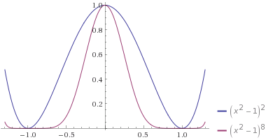
The case $W^{\prime\prime}(\pm 1)=0$ is conceptually more complicated since, from the physical point of view, if $W$ is “too flat”, then the system might develop “approximative or intermediate phases”. The extreme case of this would be, for instance, the case in which $W(\tau)>0=W(\sigma)$ for any $\tau\in(-a,a)$ and any $\sigma\in[-1,-a]\cup[a,1]$, with $a\in(0,1)$: in this situation, minimizers would prefer the state parameters $\pm a$ rather than $\pm 1$ and the state parameters with value in $(a,1]$ (as well as in $[-1,-a)$) become empty, thus violating the density estimates.

Interestingly, non-degeneracy assumptions on the potentials also play an important role in the asymptotic theory of critical points in terms of the limiting varifold, see in particular Assumption A on page 51 of [MR1803974] (moreover, a different growth from the potential wells can also create different phenomena in other settings, see e.g. [MR3385194] for the case of singular potentials).

The goal of this paper is to provide density estimates for degenerate potentials, namely when $W^{\prime\prime}(\pm 1)=0$, under weaker growth assumptions. The method of the proof is very general, it also applies to quasiminima, and we can deal with an energy functional, which is possibly non-quadratic in the gradient term (and so corresponding also to quasilinear PDEs), that we now introduce in details.

Given $n\in\mathbb{N}$, $n\geqslant 1$, and a bounded, open set $\Omega\subset\mathbb{R}^{n}$, we consider an energy functional of the form

We suppose that, for any $x\in\mathbb{R}^{n}$, $\tau\in\mathbb{R}$ and $\xi\in\mathbb{R}^{n}$, it holds that

for some $\theta\in(-1,1)$, $\lambda\in(0,1]$, $\Lambda\in[1,+\infty)$, $p\in(1,+\infty)$ and ${{m}}\in(p,+\infty)$.

Roughly speaking, conditions (1.3) and (1.4) mean that the energy density under consideration is bounded from both sides by a “gradient term of $L^{p}$-type” and, in the vicinity of a fixed phase (say, the phase corresponding to $-1$), by “a well which grows like a power $m$” (when $p=2$, the degeneracy of the potential reflects¹¹ 1 As a technical observation, we observe that we will focus our analysis on each separate well of the potential. In this way, our result in Theorem 1.1 also applies to double well-potentials in which only one of the two wells possesses a growth condition as in (1.7). into the fact that $m>2$, see Figure 1).

Given $Q\in[1,+\infty)$, we say that $u\in W^{1,p}(\Omega)$ is a $Q$-minimum in $\Omega$ if, for any open and bounded set $\Omega^{\prime}\Subset\Omega$, we have that ${\mathscr{E}}_{\Omega^{\prime}}(u)<+\infty$ and

for any $v\in W^{1,p}(\Omega^{\prime})$ with $u-v\in W^{1,p}_{0}(\Omega^{\prime})$.

Of course, when $Q=1$, the notion in (1.5) boils down to local minimality. In the framework of (1.5) (and denoting, as customary, the $n$-dimensional Lebesgue measure by ${\mathscr{L}}^{n}$), our main result is the following:

From Theorem 1.1, we obtain the following general density estimate:

As a consequence of Corollary 1.9 we also have a convergence result in the Hausdorff distance:

We notice that conditions (1.13) and (1.14) are just a rephrasing of (1.3) and (1.4) that take into account the growth from both the wells of the potential that induces the two phases $1$ and $-1$.

Next section is devoted to the proof of the main result of Theorem 1.1. Then, the simple proofs of Corollaries 1.9 and 1.10 will be given in Sections 3 and 4, respectively.

We fix an additional parameter $T\in(0,+\infty)$, which will be suitably chosen, possibly also in dependence of $\lambda$, $\Lambda$, $\theta$, $n$, ${{m}}$, $p$, $Q$, $r_{o}$ and $c_{o}$ (recall the structural constants in (1.3), (1.4) and (1.6)).

The proof of Theorem 1.1 is based on an iteration argument. To this end, for any $k\in\mathbb{N}$ and $x\in B_{(k+1)T}$, we set

From now on, $C>0$ will be a constant, which possibly depends on the structural constants $\lambda$, $\Lambda$, $\theta$, $n$, ${{m}}$ and $p$ in (1.3) and (1.4), and also on the fixed $Q$, $r_{o}$ and $c_{o}$ of Theorem 1.1, but it is independent of $T$, and can freely vary from line to line (later on, $T$ will be supposed to be sufficiently large with respect to $C$). In this way, we have that, for any $x\in B_{(k+1)T}$,

From this and (1.4), letting

we obtain that

Notice now that

and therefore, by the definition of $\Omega_{k}$ in (2.3) and that of $v_{k}$ in (2.1), we have that $v_{k}=u$ on $\partial\Omega_{k}$. Hence, the $Q$-minimality of $u$ (recall (1.5)) implies that

Using this, (1.3) and (2.4), it follows that

On the other hand, by Young’s Inequality (with exponents $p$ and $\frac{p}{p-1}$) and Coarea Formula, for any Lipschitz function $w$ we have that

Moreover, from (2.1),

In particular, choosing $T$ conveniently large, it holds that

As a consequence, we have that

for any $t\in\left[\frac{\theta-1}{2},\,\theta\right]$.

In particular, by (2.3),

for any $t\in\left[\frac{\theta-1}{2},\,\theta\right]$.

In addition, recalling (2.5), we have that $(\partial B_{(k+1)T})\cap\{u>t>v_{k}\}\subseteq\{v_{k}=1\geqslant u\}\cap\{u>v_{k}\}$ and so

Consequently,

Now we observe that, by Isoperimetric Inequality,

This and (2.10) imply that

Accordingly, using first (2.11), and then (2.7), with $w:=u$ and $w:=v_{k}$, we conclude that

This and (2.9) imply that

Consequently, recalling (2.2) and (2.6), we find that

Furthermore, exploiting (2.6), we see that

As a consequence of this, and recalling (2.3) and (2.8), we have

Now we define

With this, we can rewrite (2.12) and (2.13) as

We remark that, in view of (2.1) and (2.14),

On the other hand, from (2.14) and the fact that $v_{k}(x)\in[-1,1]$ in $B_{(k+1)T}$,

Now we insert this information and (2.16) into (2.15) and we obtain that

It is now convenient to introduce the following quantities (somehow reminiscent of “area” and “volume” terms):

With this notation, we can rewrite (2.17) as

Now we let $\varepsilon$ be the structural constant²² 2 We take this opportunity to amend a typo in [FV]: the left-hand side of (61) there should be “${\mathscr{V}}_{k}^{{(n-1)/n}}+{\mathscr{A}}_{k}$” instead of “${\mathscr{V}}_{k+1}^{{(n-1)/n}}+{\mathscr{A}}_{k+1}$”. in Lemma 12 of [FV]. Exploiting (1.7), for $T$ large enough we have that $T^{n-\frac{pm}{m-p}}\leqslant\varepsilon$. This and (2.18), together with (1.6), imply the hypotheses of Lemma 12 in [FV], which in turn implies that

for some constant $c>0$, and this proves (1.8). $\Box$

The proof of (1.10) is standard (for instance, one can repeat verbatim the proof of Lemma 10 in [FV]).

The proof of (1.12) is also a simple consequence of (1.10) and Theorem 1.1: we provide full details for the facility of the reader. We define $\theta_{\star}:=\min\{\theta,\vartheta\}$. Since $\theta_{\star}\in(-1,\theta]$, the structural assumptions in (1.3) and (1.4) hold true with $\theta$ replaced by $\theta_{\star}$. In addition, since $\theta_{\star}\leqslant\vartheta$ we have that $\{u>\vartheta\}\subseteq\{u>\theta_{\star}\}$ and thus, by (1.11),

These considerations imply that we can exploit Theorem 1.1 with $\theta_{\star}$ replacing $\theta$. In this way, from (1.8) we deduce that, for large $r$,