A new class of fuzzy spaces with classical limit

The fuzzy spaces presented below are more precisely series of matrix algebras, numbered by the size $N$ of the matrices $\hat{X}_{N}^{\alpha}$. The entries of the matrices $\hat{X}_{N}^{\alpha}$ are determined from specific values of the Fourier components of a function $x^{\alpha}$ on a manifold immersed in $\mathbb{R}^{d}$. (see (2.6) and (4.2) below). These series, are matrix regularizations according to [8], i.e. the classical limit of these series of matrix algebras is the space of functions on the manifold immersed in $\mathbb{R}^{d}$.

The definition of a matrix regularization according to [8] is the following: Let $Q_{N}$ be a series of linear maps from a space of functions on a manifold $M$ with functions $f$ (here functions on a submanifold of $\mathbb{R}^{d}$) to Hermitian $N\times N$-matrices $Q_{N}(f)$. Then the $Q_{N}$ are a matrix regularization, when

1. 1.

   The matrices $Q_{N}(f)$ converge in matrix norm, i.e. for a function $f$

   $$\lim_{N\rightarrow\infty}\left\|Q_{N}(f)\right\|<\infty$$

   (2.2)

   (for example, $\left\|\hat{f}\right\|=\max_{1<n<N}\sum_{n=1}^{N}\left|f_{nm}\right|$for a matrix $\hat{f})$.

2. 2.

   The matrix multiplication converges to the ordinary product of functions, i.e. for For two functions $f$, $g$

   $$\lim_{N\rightarrow\infty}\left\|Q_{N}(f)Q_{N}(g)-Q_{N}(fg)\right\|=0$$

   (2.3)

3. 3.

   For differentiable functions $f$, $g$ the commutator converges to a Poisson bracket

   $$\lim_{N\rightarrow\infty}\left\|-i\beta(N)[Q_{N}(f),Q_{N}(g)]-Q_{N}(\{f,g\})\right\|=0$$

   (2.4)

   i.e. the manifold is a Poisson manifold. The function $\beta(N)$ should have the property to converge to a constant for $N\rightarrow\infty$.

Due to the last property, a matrix regularization can be seen as a special kind of quantization in the sense of quantum mechanics, at least, when the Poisson bracket is none-degenerate. In this case, the manifold becomes a symplectic manifold and functions on the symplectic manifold are mapped by the regularization to operators in a way that the commutator of two functions is nearly the regularization of the Poisson bracket induced by the symplectic structure.

We also introduce “convergence within border” and “equivalence within border” for matrices. To define this, let $\delta$ be small compared to $N$ and let $\hat{f}_{\delta}$ be the matrix, where the outer border of size $\delta$ has been set to $0,$ i.e. $\hat{f}_{\delta,nm}=\hat{f}_{nm}$ for $\delta<n,m<N-\delta$ and $\hat{f}_{\delta,nm}=0$ for $n,m\leq\delta$ and $N-\delta\leq n,m$.

We say that a matrix $\hat{f}_{N}$ converges within the border $\delta$, when $\lim_{N\rightarrow\infty}\left\|\hat{f}_{N,\delta}\right\|$ converges. Equivalently, we also can use a weaker kind of matrix norm, which only accounts for matrix entries within the border, such as $\left\|\hat{f}\right\|=\max_{\delta<n<N-\delta}\sum_{n=\delta}^{N-\delta}\left|f_{nm}\right|.$ Analogously, we say that two matrices $\hat{f}$ and $\hat{g}$ are equivalent within the border $\delta$, when $\hat{f}_{\delta}$=$\hat{g}_{\delta}$. With such definitions, we are able to account for fuzzy spaces that in a sense have a manifold with border as classical limit.

A simple example of a fuzzy space is the fuzzy cylinder (see [6, 11]). Generalizations of the fuzzy cylinder will play an important role in the following. The fuzzy cylinder is based on a mapping from functions to Toeplitz matrices, i.e. matrices in which each descending diagonal from left to right is constant.

A basis for Toeplitz matrices are $N\times N$-matrices $\hat{e}_{a,N}$ with only $1$ on the $a$.th diagonal, i.e.

where $a$ can be an integer between $-N+1$ and $N-1$. For example, $\hat{e}_{0}$ is the unit matrix. On the other hand let $f(\varphi)=\sum f_{n}e^{in\varphi}$ be the Fourier series of the function $f$. The mapping from functions to matrices via

preserves multiplication of functions for $N\rightarrow\infty$, since $Q_{\infty}(e^{in\varphi})Q_{\infty}(e^{im\varphi})=\hat{e}_{n}\hat{e}_{m}=\hat{e}_{n+m}=Q_{\infty}(e^{i(n+m)\varphi})$ and therefore

for two functions $f$ and $g$. The linear operators $Q_{N}$ are a matrix regularization as defined above. In the remaining, we will often indicate functions in the function space by its arguments, such as $f(\varphi)$, and the corresponding regularized matrices with a hat, such as $\hat{f}$.

The generalized fuzzy cylinder is defined in the following way. Let $x(\varphi)$ and $y(\varphi)$ be two functions that define a closed curve in $\mathbb{R}^{2}$ and let $x(\varphi)=\sum x_{n}e^{in\varphi}$ and $y(\varphi)=\sum y_{n}e^{in\varphi}$ be their Fourier series. Then the matrices replacing the coordinate functions are defined via

Since $\hat{x}_{N}$ and $\hat{y}_{N}$ are Toeplitz-matrices, they commute, i.e. $[\hat{x}_{N},\hat{y}_{N}]=0.$ When we further assume that $x_{n}=0$ and $y_{n}=0$ for $n>\delta$, where $\delta$ is small compared to $N$, then the commutators with $\hat{z}$ fulfill

within the border $\delta$. For $N\rightarrow\infty$ the algebra generated by the matrices converge in the sense of (2.2), (2.3) and (2.4) within the border $\delta$ to an algebra of functions on a submanifold of $\mathbb{R}^{3}$, which is the product of the curve defined by $x(\varphi)$ and $y(\varphi)$ times the interval $[0,\beta]$. This manifold has the natural Poisson-bracket

It is also possible to start in (2.8) with $\hat{x}_{\infty}$ and $\hat{y}_{\infty}$ and use $\hat{z}_{\beta}=\sum_{n}\beta n\left|n\right\rangle\left\langle n\right|$. When we let $\beta$ got to $0$, the classical limit is the curve defined by $x(\varphi)$ and $y(\varphi)$ times $\mathbb{R}$. However, in this case, the definitions (2.2), (2.3) and (2.4) have to be extended to operators on a Hilbert space.

For a further generalization of the fuzzy cylinder, we start again with a function defined by a Fourier series, which however depends on a second parameter

with $q\in[q_{1},q_{2}]$ a finite interval and $\varphi\in[0,2\pi]$. We note that, when the Fourier series is truncated at a specific $n$, for example for $|n|<\delta$ the function $f$ is approximated by the truncated Fourier series. In the following it is assumed that $f_{n}=0$ for $\left|n\right|\geq\delta$ for a constant $\delta$ that is small compared to $N$.

A matrix regularization $Q_{N}(f)$ for the function $f$ is defined with the $N\times N$-matrix

where $\hat{e}_{nm}=\left|n\right\rangle\left\langle m\right|$. This definition can be extended to “infinite dimensional” matrices, i.e. $N=\infty$. Also with $N=\infty$, criteria (2.2) is fulfilled, due to the $\delta$-condition. When $f$ does not depend on $q$, definition (2.12) reduces to the regularization (2.6) of the generalized fuzzy cylinder.

$q(n,m)$ is a discretizing function, which assigns the matrix entry $\hat{e}_{nm}$ to a point in the interval of $q$. $q(n,m)$ should have to following properties:

• •

  It should fill out the interval for $q$: $q(0,0)=q_{1}$, $q(N,N)=q_{2}$ (as for large $N$ $q(0,0)\approx q(1,1)$, we can take $q(0,0)$ instead of $q(1,1)$, which renders the formulas for the examples for $q(n,m)$ below less complex).

• •

  It should depend “smooth” on its arguments, i.e $q(m,p)=q(m,n)+\frac{\beta}{N}(p-n)$ for $p-n$ small compared to $N$ and some constant $\beta$ that can depend on $m$,$n$ and $p$. Analogously, $q(p,n)=q(m,n)+\frac{\beta}{N}(p-m)$ for $p-m$ small compared to $N$ .

• •

  Examples are $q(n,m)=\frac{q_{2}-q_{1}}{2N}(m+n)+q_{1}$ (in this case $\beta=\frac{1}{2}$) or $q(n,m)=\frac{q_{2}-q_{1}}{N}n+q_{1}$ (in this case $\beta=1$ for the left argument and $\beta=0$ for the right argument).

When the function $f$ is real-valued, the resulting matrix $Q_{N}(f)$ is Hermitian for a symmetric discretizing function $q(m,n)=q(n,m)$, since for a real-valued function, the coefficients of the Fourier series have the property that $\bar{f}_{n}=f_{-n}$.

Analogously to [10], we can now evaluate the matrix product of two matrices $\hat{f}$ and $\hat{g}$ as defined in (2.12), which have one times differentiable Fourier coefficient functions $f_{n}(q)$ and $g_{n}(q)$

where in the last step all functions are evaluated at $q=q(n,m)$. Since

the last equation is equivalent to

It follows that the commutator of such regularized functions can be approximated by the Poisson bracket of the functions

Thus, all three criteria (2.2), (2.3), (2.4) above are fulfilled. Note that the Poisson bracket of the classical limit is $\{q,\varphi\}=-1$, which also follows from $[\hat{q},Q_{N}(e^{i\varphi})]=\frac{1}{N}Q_{N}(e^{i\varphi})$.

When the coefficient functions $f_{n}(q)$ and $g_{n}(q)$ are only continuous, one can show that $Q(f)Q(g)=Q(fg)+\mathcal{O}\left(\frac{1}{N}\right)$ and $[Q(f),Q(g)]=\mathcal{O}\left(\frac{1}{N}\right)$, i.e. the criteria (2.2), (2.3) are still fulfilled.

From (2.14) one sees that the Fourier coefficients $f_{n}$ for $n\rightarrow\infty$ need to go to $0$ faster than $\frac{1}{n}$, which is the case for functions with $f_{n}=0$ for $\left|n\right|\geq\delta$. However, also other functions, like functions twice differentiable in $\varphi$ and specific piece wise continuous functions (but not all) have this property. In (2.13) only the differentiability in $q$ was used. As long as the Fourier coefficients go to $0$ as fast such that (2.13) is fulfilled, (2.12) defines a matrix regularization. Thus, it is possible to start with functions $x(q,\varphi)$ and $y(q,\varphi)$, which do not define a closed curve for a specific $q$, but which only have Fourier coefficients, which go to $0$ fast enough. In this case, it would be better to talk of a fuzzy immersed strip. The same applies to the generalized cylinder as described in the previous section.

Up to now, we have ignored, what happens at the borders $q=q_{1}$ and $q=q_{2}$. Due to the discretizing function $q(n,m)$, which maps values at the border of the $q$-interval to the border of the matrices, we have to look at $n<\delta$ and $N-n<\delta$. We see that formula (2.15) is only valid within the border $\delta.$ This problem can be avoided, when the coefficient functions $f_{n}(q)$ and $g_{n}(q)$ go to zero at the border, i.e. when $f_{n}(q_{1})=f_{n}(q_{2})=0$. This can be seen by embedding a matrix of size $N$ in a bigger zero matrix, resulting in a border of zeros surrounding the original matrix. The continuation of functions $f_{n}(q)$, which do not go to zero at the border, into this border would result in non-continuous extended functions, which are not differentiable.

When we demand that $f(q_{1},\varphi)=f(q_{2},\varphi)=0$, the submanifolds that can be regularized with $Q_{N}$ have to be immersions of a cylinder into $\mathbb{R}^{d}$ with ends shrunk to a point. When the submanifold has a border, the $Q_{N}$ only converge within border.

When the target space is $\mathbb{R}^{3}$, a two-dimensional immersed submanifold can be parametrized by the three functions

The fuzzy space defined by matrix regularization of these functions with $N\times N$-matrices is then

In this section we give an example based on the fuzzy immersed cylinder that later on will be generalized to a fuzzy manifold having the structure of a string vertex. Here, we construct the part of the vertex, which at one end with respect to the $z$-direction has a circular cross-section and transforms along the $z$-direction into a cross-section similar to an 8. The center crossing of the eight is the point, where the string vertex splits into two cylinders.

To define the fuzzy "circle-to-eight”-space let us start with two coordinate functions in polar coordinates, i.e. $x(z,\varphi)=r(z,\varphi)\cos\varphi$ and $y(z,\varphi)=r(z,\varphi)\sin\varphi$ with $r(z,\varphi)=r_{1}(z)+r_{2}(z)\cos 2\varphi$. This is equivalent to

With $r_{1}(z)=1$ and $r_{2}$ continuously increasing between $z_{1}$ and $z_{2}$ and $r_{2}(z_{1})=0$ and $r_{2}(z_{2})=1$ the corresponding immersed manifold has a transition from a circle to a 8 as shown to the left of Fig. 1.

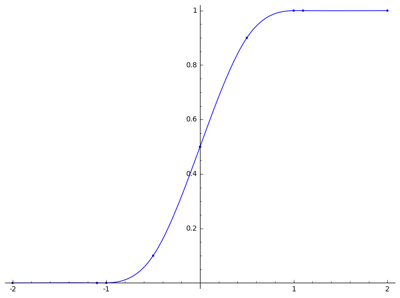
To fix the functions $r_{1}$ and $r_{2}$ between $z_{1}$ and $z_{2}$, we need a continuously increasing, differentiable function $h(q)$ with $h(q<-1)=0$ and $h(q>1)=1$. For the figures and matrices in this article, this function is always represented with a cubic spline interpolating the points $(-1,0)$, $(-0.5,0.1)$, $(0,0.5)$$,(0.5,0.9)$ and $(1,1)$ with further support points at $h=0$ and $h=1$ outside of $-1$ and $1$. The spline $h$ with it support points (and the function $r_{2}$, which is here equivalent to $h$) is shown to the right of Fig. 1.

A matrix regularization according to (2.12) for the manifold shown in Fig. 1 is

Here, $z=1+2q$ and $q$ is discretized with $-1+\frac{2n}{N}$. Again, as the ends of the circle-to-eight manifold are not closed, the algebra defined by these matrices only converges within border in the sense of (2.2) to (2.4). Completely converging matrices can be formed by providing the ends with “caps”, for example by fading out the Fourier coefficients in an interval larger than $[-1,1]$ and extending the matrices correspondingly.

Fig. 2 shows a visualization of the matrices $\hat{x}$, $\hat{y}$ and $\hat{z}$ with $N=30$ in the form of “dot matrix diagrams”. Every matrix is represented by a matrix of circles. Every circle represents a matrix entry and has a radius proportional to the root of the absolute value of the respective matrix entry. Matrix entries equal to $0$ are depicted with a small point, such that the rows and columns can be better identified. We will use these dot matrix diagrams in the following for more complicated examples. They represent an easy way to visually compare properties of matrices with each other.

In general, let us assume that we have two (or more general $S$) matrices $\hat{f}_{a}$, which are regularizations of the functions $f_{a}(q,\varphi).$ The direct product of these matrices is the matrix $\hat{F}$ with $F_{ab,nm}=f_{a,nm}\delta_{ab}$, where we have introduced a double-index notation with $a,b=1\ldots S$ and $i,j=1\ldots N$. For example, with $S=2$

Due to the invariance of a fuzzy space with respect to permutations (being a special kind of unitary transformation), we also can exchange the role of the “inner” and the “outer” indices

where $\hat{P}$ is a suitable permutation. The matrix $\hat{F}^{\prime}$ can be seen as a regularization of a matrix-valued function $F$

From now on, we will consider $\hat{F}^{\prime}$ and $\hat{F}$ as equivalent. In summary, we have transformed the regularization of the two real-valued functions $f_{1}$ and $f_{2}$, which are defined on the cylinder (or more general strip) $[q_{l},q_{r}]\times[0,2\pi]$ to a regularization of one matrix-valued function $F$ defined on this cylinder.

Due to (3.3), the borders of the matrices $\hat{f}_{a}$ also have been shifted to the border of the matrix $\hat{F}$. Thus, when we have matrices converging in border then also their direct product permuted according to (3.3) converges in border.

The coordinate functions $x_{1}^{\alpha}(q,\varphi)$ and $x_{2}^{\alpha}(q,\varphi)$ used for defining the matrices of two fuzzy spaces by regularization can be composed into matrices $X^{\alpha}(q,\varphi)$ according to (3.4). When a constant unitary transformation $U$, i.e. a unitary transformation independent of $q$ and $\varphi$ is applied to the matrix-valued functions $X^{\alpha}(q,\varphi)$, this is equivalent to applying the unitary transformation

(which can be seen as the regularization of the matrix $U$) to the corresponding regularization $\hat{X^{\alpha}}$(3.1). In this case, multiplication of matrices commutes with regularization

On the other hand, when we start with a set of general matrix-valued functions $X^{\alpha}(q,\varphi)\in M_{N}(\mathbb{C})$, such as

and the matrices $X^{\alpha}(q,\varphi)$ are simultaneously diagonalizable with a constant unitary transformation, we can associate a direct sum of fuzzy spaces to the matrix regularization. Due to to the matrix form of the defining functions $X^{\alpha}(q,\varphi)$, a new class of symmetry is present, namely constant $U(n)$-transformations, which can be seen as a generalization of the trivial $U(1)$ symmetry of single-valued functions. After defining a regularization for general matrix-valued functions, we will also see that this symmetry can be generalized to coordinate dependent $U(n)$-transformations.

An interesting case is, when one of the matrix-valued functions $Z(q,\varphi)$ is proportional to the unit matrix, i.e. $Z_{ab}=z(q,\varphi)\delta_{ab}$. Fuzzy spaces based on direct sums have this property, when the same diagonal matrix for the $z$-coordinate is used for both spaces. In this case, a residual symmetry remains that can be used to transform the other matrices $\hat{X}^{\alpha}.$ Every unitary transformation $\hat{U}$ (3.5) based on a constant unitary transformations $U$ leaves the matrix $\hat{Z}$, see (3.3), invariant.

For example, we can consider the unitary transformation

which has the property that it mixes the diagonal and off-diagonal elements of the matrix-valued function $F=\left(\begin{array}[]{cc}f_{11}&f_{12}\\ f_{21}&f_{22}\end{array}\right)$

Such a transformation will below become important for two symmetric fuzzy spaces, which have the property that $x_{1}^{\alpha}(q,\varphi)=-x_{2}^{\alpha}(q,\varphi)$ for the coordinate functions except $z(q,\varphi)$. In this case, the transformation results in a swap between diagonal entries and off-diagonal entries.

We will call this “interlacing” of fuzzy spaces.

We will apply the preceding discussion to the direct sum of two generalized fuzzy cylinders. In particular, the part of the string vertex, which follows the circle-to-eight manifold (2.19), consists of two cylinders, which move away from each other with increasing $z$. In chapter 5, the fuzzy circle-to-eight space will be connected with the two interlaced fuzzy cylinders, which are defined here.

Firstly, more generally, we consider two cylinders, which are aligned along a center $\left((x_{i,0}(z),y_{i,0}(z)\right)$ ($i=1,2$ enumerates the two cylinders) and which have two $z$-depend radii $r_{i,x}(z),\text{ }r_{i,y}(z)$ along the $x$-direction and the $y$-direction. A matrix regularization for each cylinder is

The direct sum (3.1) of these two fuzzy spaces is

The $2\times 2$-matrix-valued functions (3.4) for regularization are

When the two cylinders are symmetric with respect to the $z$-axis, this implies $x_{0}(q)=-x_{1,0}(q)=x_{2,0}(q)$ and $r_{x/y}(q)=-r_{1,x/y}(q)=r_{2,x/y}(q)$. The interlaced form (3.10) of the matrices becomes

Fig. 3 shows dot matrix diagrams of matrix regularizations with $N=15$ for the two cylinders. The first row of diagrams shows the matrices $\hat{X},$$\hat{Y}$and $\hat{Z}$ for the pure direct sum of the two fuzzy cylinders, according to (3.2). The second row shows the matrices $\hat{X}^{\prime},$$\hat{Y}^{\prime}$and $\hat{Z}^{\prime}$ after a permutation according to (3.3) The third row shows the interlaced matrices according to (3.3) adjoined with (3.5) based on (3.8). If one compares Fig. 2 above for the circle-to-eight fuzzy space with the third row of Fig. 3, one sees, that the same diagonals of the matrices only have entries different from $0$. In chapter 5 we will develop a method, how these two matrices for one coordinate can be smoothly interconnected with each other.

In the following, we assume that the Fourier coefficients $F_{ab,n}(q)$ of $F$ are one times differentiable with respect to $q.$ This always can be achieved for a regularization, by interpolation the points $q(n,n)$ with a one times differentiable function. Analogously to (2.12), we assume that the $F_{ab,n}(q)$ are again $0$ for $\left|n\right|\geq\delta$, where $\delta$ is a constant that is small compared to $N$.

As in the case of the immersed cylinder (see (2.13)), we now can evaluate the matrix product of $\hat{F}$ with a further matrix $\hat{G}$, which is a matrix regularization of a matrix-valued function $G_{ab}(q,\varphi)$.

References

- [1] S. Doplicher, K. Fredenhagen, J. Roberts , The Quantum structure of space-time at the Planck scale and quantum fields, Commun. Math. Phys. 172 (1995) [hep-th/0303037]
- [2] A. Connes, Non-commutative geometry, Boston, MA: Academic Press, 1994
- [3] J. Madore, An Introduction to Noncommutative Differential Geometry and its Physical Applications, 2nd edition, Cambridge University Press, 1999
- [4] N. Ishibashi, H. Kawai, Y. Kitazawa, and A. Tsuchiya, A Large N reduced model as super- string, Nucl. Phys. B498 , 467 (1997), [hep-th/9612115]
- [5] T. Banks, W. Fischler, S. H. Shenker, and L. Susskind, M theory as a matrix model: A Conjecture, Phys. Rev. D55 , 5112 (1997), [hep-th/9610043]
- [6] H. Steinacker, Non-commutative geometry and matrix models, PoS QGQGS 2011 (2011) 004 [arXiv:1109.5521 [hep-th]]
- [7] J. Madore, The Fuzzy sphere, 1991, Class.Quant.Grav. 9 (1992) 69-88
- [8] J. Arnlind, J. Hoppe, G. Huisken, Multi-linear formulation of differential geometry and matrix regularizations J.Diff.Geom. 91 (2012) no.1, 1-39 [arXiv:1009.4779 [math.DG]]
- [9] J. Arnlind, M. Bordemann, L. Hofer, J. Hoppe and H. Shimada, Fuzzy Riemann surfaces, JHEP 0906 (2009) 047 [hep-th/0602290]
- [10] H. Shimada, Membrane topology and matrix regularization, Nucl. Phys. B 685 (2004) 297 [hep-th/0307058]
- [11] A. Sykora, The fuzzy space construction kit, Oct 3, 2016. 26 pp. [arXiv:1610.01504 [hep-th]]
- [12] SageMath, the Sage Mathematics Software System (Version 7.0), 2016, [http://www.sagemath.org]