Multipolar second-harmonic generation by Mie-resonant dielectric nanoparticles

Being stimulated by a rapid progress in nanofabrication techniques, dielectric resonant nanostructures with high refractive index are currently employed in various applications of nanophotonics, offering competitive alternatives to plasmonic nanoparticles [1]. Advantageous optical properties of high-index dielectric nanoparticles, such as low dissipative losses, optical magnetic response, and multipolar resonances, imply exclusive capabilities for light manipulation at subwavelength scales, especially in the nonlinear regime [2].

Acting as optical nanoantennas, high-permittivity dielectric nanoparticles exhibit strong interaction with light due to the excitation of both electric and magnetic Mie resonances they support. Compared to plasmonic nanoscale structures, where the electric field is strongly confined to surfaces, the electric field of the resonant modes in dielectric nanoparticles penetrates deep inside their volume, thus enhancing intra-cavity light-matter interactions in a bulk material. Such a strategy of utilizing the Mie resonances in the subwavelength dielectric geometries has been recently recognized as a promising route for improving the nonlinear conversion processes at the nanoscale [3, 4, 5, 6, 7, 8, 9] .

Second-harmonic generation in plasmonic nanostructures is known to be governed mainly by surface nonlinear response, which can be enhanced at the geometric plasmon resonances [10, 11, 12, 13, 14, 15, 16, 17, 18, 19, 20]. Primarily, electric dipole response associated with the surface plasmon resonance is most widely exploited for deeply subwavelength metallic particles and their composites, and the nonlocal bulk contribution to second-harmonic generation (SHG) is largely ignored [21, 22]. The excitation of multipolar resonances driven by displacement currents in dielectric nanostructures can significantly reshape the nonlinear scattering, in particular, due to the bulk nonlinear response altered with the field gradients distributed over the volume. One of the most promising material for implementation of all-dielectric nanophotonics is silicon due to its CMOS compatibility and strong optical nonlinearities [23, 24]. In particular, silicon was employed in most of works on the trapped magnetic dipole resonances [25, 26] and the associated enhancement of the third-order nonlinear processes [3, 27, 4, 6, 28]. Though silicon, both crystalline and amorphous, is a centrosymmetric material, and thus, similar to noble metals, its bulk second-order nonlinear response is inhibited [29], the light confinement and enhancement due to excitation of the resonant modes increases the efficiency of the frequency conversion, and quite high yield of SHG from individual nanowires [30, 31] and nanoparticles [32] can be achieved.

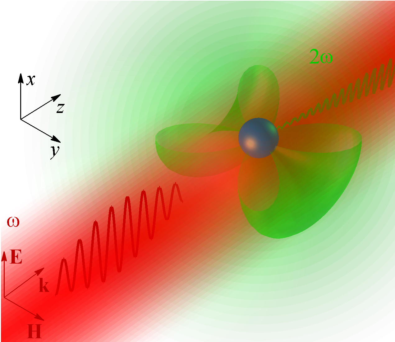
In this paper, we investigate the characteristic features of SHG from dielectric nanoparticles made of high-index centrosymmetric materials and optically excited in the vicinity of the pronounced low-order Mie resonances, with a particular focus on the magnetic dipole resonance. We take into account the contributions of both surface and bulk induced nonlinear sources described in the framework of the phenomenological model [33, 30, 31]. We reveal that the SH radiation is dominated by dipolar and quadrupolar contributions, specifically by two axially symmetric electric quadrupoles (oriented along the magnetic and electric fields, respectively, in the incident wave), an electric dipole (directed along the wave vector of the incident wave), and a magnetic quadrupole. We emphasize that the case we study is essentially distinct from the Rayleigh limit, small plasmonic particles and Rayleigh-Gans-Debye model, or first Born approximation (assuming a low refractive-index mismatch between the interior of the particle and a host medium) [11, 34, 35]. By contrast, in the small-particle limit the SH field is described by one electric quadrupole and one electric dipole [11]. In the experimental study [34], it is further discussed that the octupolar traits in SH scattering diagrams appear for the nonresonant polysterene nanoparticle as corrections compared to the Rayleigh-limit SHG [11] as a consequence of increasing the size parameter.

Here we derive the excitation coefficients of the nonlinearly generated multipoles with an original procedure based on the use of the Lorentz lemma. It can be regarded as a more practical alternative to the nonlinear Mie theory analysis [11, 36, 12, 16]. Our approach can be applied to Mie-resonant nanoparticles made of not only centrosymmetric but also noncentrosymmetric high-index materials actively employed for nonlinear nanophotonics [9, 37, 38, 39]. In addition, we provide a detailed analytical solution for the resonantly enhanced SHG driven by the pronounced magnetic dipole excitation with the approach outlined in Ref. [5]. The validity of the developed theory and analytically described multipolar expansion of the SH field is confirmed in the direct full-wave numerical calculations.

We consider a high-permittivity spherical dielectric particle of radius $a$, excited by the linearly-polarized plane wave ${\bf E}({\bf r})=\hat{{\bf x}}E_{0}e^{ik_{0}z}$ propagating in the $z$ direction, as illustrated schematically in Fig. 1. The analysis we perform also gives a qualitatively correct picture of the second-harmonic (SH) fields generated by an arbitrary single-scale nanoscale object (e.g., a finite-extent nanorod whose cross-sectional diameter is of the order of its length). The particle is characterized by the frequency-dependent dielectric constant $\varepsilon(\omega)$. The homogeneous host medium is air. The problem of linear light scattering by a sphere is solved using the multipole expansion in accord with Mie theory. The resultant scattering efficiency is plotted in Fig. 2 for a silicon nanoparticle excited at wavelength $\lambda_{0}=1050$ nm in the range of radii featuring MD and ED resonances.

In the frequency range between the magnetic (MD) and electric (ED) dipolar resonances, the electric field at the fundamental frequency inside the nanoparticle is well approximated by a superposition of only MD and ED modes, as evidenced by Fig. 2

where $k(\omega)=k_{0}\sqrt{\varepsilon(\omega)}$ is wavenumber in the medium, $k_{0}=\omega/c$, $j_{1}(k(\omega)r)$ is spherical Bessel function of order $l=1$, ${\bf{X}}_{1,1}({\theta,\varphi})$ are vector spherical harmonics (in the spherical coordinate system associated with $z$ axis), $A_{1,1}^{E}$ and $A_{1,1}^{M}$ are coefficients known from Mie theory [40].

The pronounced character of the low-order Mie resonances is essential for many applications of high-permittivity dielectric nanoparticles in low-index environment [1, 41] and for the analysis we develop below. We specifically focus on Mie-resonant dielectric nanoparticles, whose sizes correspond to the resonant excitation of the leading magnetic dipole and electric dipole modes at the laser fundamental wavelength, as shown in Fig. 2. The analysis of SHG from high-index dielectric nanoparticles exhibiting dipolar resonances is important for modern nanoscale optics, given the increasing interest in the rapidly expanding field of all-dielectric nanophotonics and growing number of nonlinear experiments being currently done by many research groups worldwide exactly under the conditions associated with resonant excitation of the low-order Mie modes [2].

The second-order polarization for the particles made of centrosymmetric homogeneous materials can be written as a superposition of dipolar surface (local) and quadrupolar bulk (nonlocal) contributions [42, 43, 33, 30, 31]

where $E_{r}^{(\omega)}$ and $E_{\tau}^{(\omega)}$ are the radial and tangential components of the electric field on the spherical surface, $\bf{\hat{r}}_{0}$, $\bm{\hat{\tau}}_{0}$ are the corresponding unit vectors. The coefficients $\gamma$, $\beta$, $\delta^{\prime}$, $\chi^{\left({2}\right)}_{\bot\bot\bot}$, $\chi^{\left({2}\right)}_{\bot\parallel\parallel}$, $\chi^{\left({2}\right)}_{\parallel\bot\parallel}$ are material parameters of the dielectric, the $\beta$ term vanishes in the bulk, $\nabla\cdot{\bf{E}}^{(\omega)}=0$, due to the homogeneity of the material, $\delta(\tilde{r})$ is the Dirac delta function, and step function $\Pi(\tilde{r})$ is defined by $\Pi(\tilde{r})=\left\{0,\tilde{r}<0;1,\tilde{r}>0\right\}$. Importantly, the $\gamma$ term exhibits a surface-like behavior, and it is often referred to as a nonseparable bulk contribution [16, 31]. We assume phenomenological model (2) qualitatively valid for amorphous and crystalline silicon nanoparticles, disregarding any anisotropy effects [33, 30, 31]. Specifics of SHG from nanocrystalline silicon nanoparticles was studied experimentally and numerically in Ref. [32]. According to Eq. (2b), the nonlinear surface sources ${\bf{P}}_{\text{surf}}^{\left({2\omega}\right)}$ are defined by the field ${\bf{E}}^{(\omega)}$ at the pump wavelength inside the nanoparticle. Introducing functions $\delta(r-a+0)$ and $\Pi(a-0-r)$ in Eqs. (2b) and (2c) allows us to formalize mathematical derivations.

Plugging Eqs. (2) into the Maxwell’s equations, the SH electromagnetic field ${{\bf{E}}^{\left(2\omega\right)}},{\bf{H}}^{\left(2\omega\right)}$ is the forced solution of a set of equations

where ${\bf j}^{({2\omega})}=-2i\omega({\bf{P}}_{\text{surf}}^{\left({2\omega}\right)}+{\bf{P}}_{\text{bulk}}^{\left({2\omega}\right)})$ is the current density induced due to the quadratic nonlinearity, and

is the dielectric permittivity distribution at the second harmonic frequency. Note, in the considered frequency range under approximation (1) the polarization sources, and consequently, the external current ${\bf j}^{({2\omega})}$ constitutes the quadratic form of the electric field ${\bf{E}}^{\left({\omega}\right)}$, which is defined predominantly by the electric and magnetic dipolar modes excited at the fundamental frequency $\omega$. Since these two modes depend linearly on sine and cosine functions of of the polar angle, multipolar expansion of the generated SH field to the leading order contains only dipolar and quadrupolar spherical harmonics.

Similar to the work [37], we analyze the induced nonlinear multipolar sources by employing general expressions for the electric and magnetic multipolar coefficients at the SH wavelength as defined by the overlap integrals of the sources with spherical harmonics [40]. Our calculations show that within the framework of approximation (1), the multipolar composition features two axially-symmetric electric quadrupolar (EQ) components, whose amplitudes are proportional to $(A_{1,1}^{E})^{2}$ and $(A_{1,1}^{M})^{2}$, as well as ED and MQ modes with amplitudes proportional to $(A_{1,1}^{E}A_{1,1}^{M})$. Thus, outside the nanoparticle, the SH magnetic field assumes the form

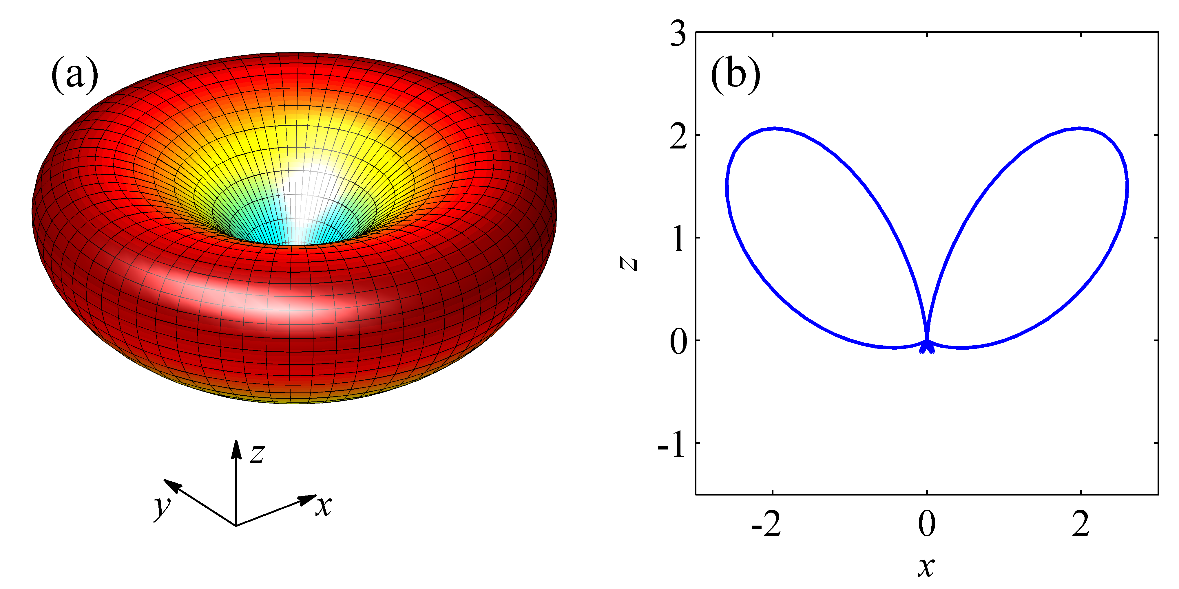
Here ${\bf{X}}_{l,m}$ are spherical functions; $({\theta,\varphi})$, $({\theta_{1},\varphi_{1}})$, $({\theta_{2},\varphi_{2}})$ are polar and azimuthal angles of the spherical coordinate systems associated with $z$, $y$ and $x$ axes, respectively, $h^{(1)}_{l}$ is the spherical Hankel function of the first kind of order $l$. In Eq. (5), the terms proportional to $q^{E}_{1}$ and $q^{E}_{2}$ describe the fields emitted by the electric quadrupoles which are axially symmetric to the $y$ and $x$ axes, the term proportional to $d^{E}$ is the radiation field of the electric dipole oriented along the propagation direction $z$ of the incident wave, and the term proportional to $q^{M}$ is due to the presence of the magnetic quadrupolar component in the source. The far-field diagrams of the generated SH multipoles,

are visualized in Fig. 3.

The excitation coefficients of the multipolar modes, $q^{E}_{1}$, $q^{E}_{2}$, $d^{E}$, $q^{M}$, are linear functions of the phenomenological parameters, $\gamma$, $\beta$, $\delta^{\prime}$, $\chi^{\left({2}\right)}_{\bot\bot\bot}$, $\chi^{\left({2}\right)}_{\bot\parallel\parallel}$, $\chi^{\left({2}\right)}_{\parallel\bot\parallel}$. Analytical expressions for the multipolar amplitudes can be found using the Lorentz lemma [44, 40]. The Lorentz lemma is widely applied in electrodynamics for calculation of amplitude coefficients of the guided modes excited by external sources and radiation diagrams of emitters. Here we show that the methodology based on the Lorentz lemma can be adopted for the analysis of the nonlinear scattering. This approach facilitates mathematical derivations, especially, in the treatment of the bulk nonlinearity, and, more importantly, it allows for generalization to nanoparticles of nonspherical shapes. For our problem, it can be formulated as follows. We introduce the auxiliary electromagnetic field $\left\{{\bf{E}}^{\left({2\omega}\right)}_{1},{\bf{H}}^{\left({2\omega}\right)}_{1}\right\}$ satisfying the Maxwell’s equations in the medium with the dielectric permittivity $\varepsilon^{(2\omega)}(r)$ in the absence of the external sources

We then apply scalar multiplication to Eqs. (3a) and (6b) by ${\bf H}^{(2\omega)}_{1}$ and ${\bf E}^{(2\omega)}$, respectively, and subtract one from another

In a similar manner, we find

Subtracting Eq. (8) from Eq. (7), we obtain

as a consequence of the Lorentz lemma. We next integrate Eq. (9) over the volume $V$, bounded by a spherical surface $S(V)$ of radius $R\gg\pi c/\omega$,

As an auxiliary solution $\left\{{\bf{E}}^{\left({2\omega}\right)}_{1},{\bf{H}}^{\left({2\omega}\right)}_{1}\right\}$, we choose the electromagnetic field, which at $r>a$ constitutes the incident and reflected multipolar electric or magnetic mode. It acquires the following form for the electric multipolar mode:

and for the magnetic multipolar mode:

Here the Hankel function of the second kind $h^{(2)}_{l}(2k_{0}r)$ corresponds to the incident spherical wave, while the Hankel function of the first kind $h^{(2)}_{l}(2k_{0}r)$ describes the reflected out-going mode. The spherical Bessel function $j_{l}(2k_{0}\sqrt{\varepsilon(2\omega)}r)$ describes the auxiliary field inside the nanoparticle. Reflection (transmission) coefficients $\eta^{E,M}_{l}$ ($t^{E,M}_{l}$) are derived from the condition of the continuity for the tangential component of the electric field and magnetic fields at the interface $r=a$:

Note that $|\eta^{E,M}_{l}|=1$ in Eq. (13).

Substituting Eqs. (11) and (12) into Eq. (10), with account for the expansion (5) and the orthogonality condition for spherical harmonics, we get the excitation coefficients of the multipolar modes at the SH frequency:

Coefficients $q^{E}_{1}$, $q^{E}_{2}$, $d^{E}$ and $q^{M}$ are in different ways related to the phenomenological parameters $\gamma$, $\delta^{\prime}$, $\chi^{\left({2}\right)}_{\bot\bot\bot}$, $\chi^{\left({2}\right)}_{\bot\parallel\parallel}$, $\chi^{\left({2}\right)}_{\parallel\bot\parallel}$. In particular, calculating the integrals in the right-hand side of Eqs. (14), one can show that

where coefficients $a_{i}$, $b_{k}$, $c_{j}$ and $f$ depend on the frequency, the particle size and the dielectric permittivity. Remarkably, the magnetic quadrupolar component $q^{M}$ depends only on one parameter $\chi^{\left({2}\right)}_{\parallel\bot\parallel}$, and, hence, it vanishes at $\chi^{\left({2}\right)}_{\parallel\bot\parallel}=0$.

At long distances from the particle, where $2k_{0}r\gg 1$, the electric field emitted at the second harmonic takes the following form:

Here, $\bm{\hat{\theta}}_{1}$, $\bm{\hat{\theta}}_{2}$, $\bm{\hat{\theta}}$ are the unit vectors directed along the increasing polar variables in spherical coordinate systems associated with the $y$, $x$ and $z$ axes, respectively, and $\bm{\hat{\varphi}}_{1}$ is the corresponding azimuthal unit vector. The study of the SH radiation pattern in different cross sections may assist in estimating the relative values of the nonlinear phenomenological parameters, $\gamma$, $\delta^{\prime}$, $\chi^{\left({2}\right)}_{\bot\bot\bot}$, $\chi^{\left({2}\right)}_{\bot\parallel\parallel}$, $\chi^{\left({2}\right)}_{\parallel\bot\parallel}$, of the quadratic nonlinearity of the dielectric material the nanoparticle is made of [30, 31].

Note, being based on Lorentz lemma, our approach can be regarded as a more practical alternative to the analysis suggested in works [45, 12, 16]. In particular, the contribution of the truly volume separable $\delta^{\prime}$ polarization source is found here not attracting a more involved treatment based on Green’s function formalism. While usually disregarded for metal nanostructures, the $\delta^{\prime}$ source dependent on spatial derivatives of the fields inside in the nanoparticle is not necessarily negligible in dielectric nanoparticles. For the surface nonlinearity, we additionally check that the excitation coefficients for the dominating SH multipoles obtained with Eqs. (14) in fact coincide with those recovered with the use of the nonlinear Mie theory for SHG from a spherical centrosymmetric nanoparticle [11, 12]. For comparison, we employed the formulas given in Supplemental Material of Ref. [12].

The interference of the nonlinearly generated multipoles could be employed for engineering the radiation directionality. Figure 4 clearly demonstrates the possibility to implement a nonlinear antenna which generates the second-harmonic light directionally. This directivity is achieved due to the excitation of the mutually perpendicular electric quadrupoles and a dipole, which are oriented along the $x$, $y$ and $z$ axes. The exemplary radiation pattern in Fig. 2 is plotted, assuming that the contribution of the magnetic quadrupole is small and the amplitudes of the ED and EQ modes in the SH radiation field are of the same order of magnitude.

Our analytical considerations are confirmed by full-wave numerical modeling performed with finite-element-solver COMSOL Multiphysics, following the procedure described in Refs. [5, 6, 9, 28, 37]. These simulations allow for solving the full scattering problem at the SH frequency using the induced nonlinear polarization within the undepleted pump approximation in the presence of the dielectric environment. Then the multipolar amplitude coefficients dependent on the geometry and a refractive-index contrast are retrieved [46]. Because the values of the phenomenological nonlinear coefficients for silicon (Si) are yet not well established and it is the subject of discussion up to now, we examined different terms in nonlinear sources (2) separately, as if they acted independently, for silicon nanoparticles exhibiting overlapped MD and ED resonances, varying the radius in the range as shown in Fig. 2. In agreement with our theoretical model, for smaller radii $a\lesssim 170$ nm the leading contributions to the radiated SH field stem from the dipolar and quadrupolar modes we distinguished, as exemplified in Fig. 5 for the nanoparticle of radius $a=145$ nm. Fig. 5 evidences that the multipolar expansion of SHG up to the order $l=2$ well approximates the total radiated power, while the higher-order corrrections $l\geq 3$ appear small. In this regime SHG process is essentially governed by two dipolar modes excited at the fundamental wavlength, because of their resonant character [Fig. 2], which distinguishes the case under study e.g. from the described in the literature SHG by small nonresonant nanoparticles and low-index-contrast polysterene nanoparticles in water [11, 34, 35]. COMSOL results additionally confirm that when defining the SH nonlinear source through the bulk and surface nonlinear polarizations, one may, to a high degree of accuracy, restrict oneself to taking into account electric and magnetic dipolar modes only. This is reasonably explained by sufficiently high quality factors of the dipolar resonances exhibiting by the high-index nanoparticles of the corresponding sizes.

We expect the total conversion efficiency to be dispersive and size-dependent. It is strongly affected by hierarchy of Mie resonances and modal overlaps, as was shown experimentally for Mie-resonant nanoparticles in the recent works [9, 32, 37]. Direct numerical simulations performed with COMSOL reveal that with increasing the nanoparticle’s size (closer to $a=200$ nm), the higher orders (up to $l=4$) show up in the multipolar expansion of the SH field. Based on the data and discussions in Refs. [47, 48, 33, 31], we approximately estimate the SHG efficiency and bulk and surface relative contributions for a silicon nanoparticle under the plane-wave illumination [Fig. 6]. For calculations, we take $\chi^{\left({2}\right)}_{\bot\bot\bot}=65\times 10^{-19}$ m²/V, and set the other nonlinearity parameters roughly of the same order of magnitude, $\chi^{\left({2}\right)}_{\bot\parallel\parallel}=\chi^{\left({2}\right)}_{\parallel\bot\parallel}=\gamma=3.5\times 10^{-19}$ m²/V. Using the polarizability model [33], we estimate $\delta^{\prime}\approx\gamma\left(\varepsilon(\omega)-4\varepsilon(2\omega)+3\right)/\left(\varepsilon(2\omega)-1\right)$. The pronounced enhancement in the second-harmonic (SH) scattering occurs near MD resonance at the pump wavelength. The dominant peaks are exhibited by $\chi^{\left({2}\right)}_{\bot\parallel\parallel}$ surface and $\gamma$, $\delta^{\prime}$ bulk sources, which we analyze in detail in Sec. III.

However, the volume response can be attributed exclusively to the separable bulk $\delta^{\prime}$ term. The mentioned above quasisurface character of the bulk $\gamma$ term [16, 31] can be inferred from Eqs. (14). Since $q^{M}$ depends only on $\chi^{\left({2}\right)}_{\parallel\bot\parallel}$, we inspect the amplitudes of electric modes $q^{E}_{1,2}$ and $d^{E}$. For the $\gamma$ source, they can be transformed to the surface integrals as follows

justifying that the bulk $\gamma$ term contributes to the effective surface response.

In this section, we consider in more detail and derive an analytical solution for SHG from a high-index dielectric particle driven by the MD mode. This particular case well describes the pronounced magnetic dipole resonance [5]. Alternatively, it may be realized in experiment by irradiating the nanoparticle with the azimuthally-polarized beam whose structure imitates the MD mode polarization distribution. In this instance, solution can be obtained from the analysis developed in Sec. II by setting $A^{E}_{1,1}=0$. However, for the sake of methodological clarity, here we take a different way and solve this basic nonlinear problem not attracting the Lorentz lemma but following the approach outlined in Ref. [5], where the third-harmonic generation by resonant silicon nanoparticles was described.

We employ a single-mode approximation and assume the fields inside the nanoparticle at $r<a$ are given by MD mode profile as follows

where $A(\omega)=E_{0}A^{M}_{1,1}\displaystyle\frac{1}{2}\sqrt{\displaystyle\frac{3}{\pi}}$. We rewrite expressions (18) in the spherical coordinate system associated with $y$ axis co-directed with the induced magnetic dipole moment:

Substituting the fields (19) into Eqs. (2), the nonlinear polarizations are recast to the surface source caused solely by the tensor component $\chi_{\bot\parallel\parallel}$,

and the bulk source consisting of two regrouped contributions

For clarity, we consider response of the structure driven by the nonlinear sources ${\bf{P}}_{\text{surf}}^{{}^{\left({2\omega}\right)}}$, ${\bf{P}}_{\text{bulk1}}^{{}^{\left({2\omega}\right)}}$ and ${\bf{P}}_{\text{bulk2}}^{{}^{\left({2\omega}\right)}}$ sequentially.

The normal surface polarization (20) in the driven Maxwell’s equations is equivalent to the dipole layer. Alternatively, in electrodynamic equations it may be formally replaced by the fictitious surface magnetic current whose density is defined by

Thus, the tangential $\theta_{1}$-component of the electric field at the spherical boundary $r=a$ undergoes a jump expressed through the derivative $\partial_{{\theta}_{1}}{{P}}_{\text{s}}^{{}^{\left({2\omega}\right)}}$:

Considering the term ${\bf{P}}_{\text{bulk1}}^{{}^{\left({2\omega}\right)}}$, which is a gradient of the scalar function, we represent the electric field as a sum of the vortex and potential vector fields

The vortex part ${\bf E}_{\text{v}}^{(2\omega)}$ is, therefore, found by solving the Maxwell’s equations with the substitution (24) transformed to

with the following boundary conditions at the nanoparticle surface

where, to account for the electric field discontinuity at the interface $r=a$, we have again introduced the surface magnetic current given by

Noticeably, the boundary conditions (23) and (26b) can be additively combined to

References

- [1] A. I. Kuznetsov, A. E. Miroshnichenko, M. L. Brongersma, Y. S. Kivshar, and B. Luk’yanchuk, “Optically resonant dielectric nanostructures,” Science 354, aag2472 (2016).
- [2] D. Smirnova and Y. S. Kivshar, “Multipolar nonlinear nanophotonics,” Optica 3, 1241 (2016).
- [3] M. R. Shcherbakov, D. N. Neshev, B. Hopkins, A. S. Shorokhov, I. Staude, E. V. Melik-Gaykazyan, M. Decker, A. A. Ezhov, A. E. Miroshnichenko, I. Brener, A. A. Fedyanin, and Y. S. Kivshar, “Enhanced third-harmonic generation in silicon nanoparticles driven by magnetic response,” Nano Lett. 14, 6488–6492 (2014).
- [4] Y. Yang, W. Wang, A. Boulesbaa, I. I. Kravchenko, D. P. Briggs, A. Puretzky, D. Geohegan, and J. Valentine, “Nonlinear Fano-resonant dielectric metasurfaces,” Nano Lett. 15, 7388–7393 (2015).
- [5] D. A. Smirnova, A. B. Khanikaev, L. A. Smirnov, and Y. S. Kivshar, “Multipolar third-harmonic generation driven by optically induced magnetic resonances,” ACS Photon. 3, 1468–1476 (2016).
- [6] A. S. Shorokhov, E. V. Melik-Gaykazyan, D. A. Smirnova, B. Hopkins, K. E. Chong, D.-Y. Choi, M. R. Shcherbakov, A. E. Miroshnichenko, D. N. Neshev, A. A. Fedyanin, and Y. S. Kivshar, “Multifold enhancement of third-harmonic generation in dielectric nanoparticles driven by magnetic Fano resonances,” Nano Lett. 16, 4857–4861 (2016).
- [7] S. Liu, M. B. Sinclair, S. Saravi, G. A. Keeler, Y. Yang, J. Reno, G. M. Peake, F. Setzpfandt, I. Staude, T. Pertsch, and I. Brener, “Resonantly enhanced second-harmonic generation using III–V semiconductor all-dielectric metasurfaces,” Nano Lett. 16, 5426–5432 (2016).
- [8] G. Grinblat, Y. Li, M. P. Nielsen, R. F. Oulton, and S. A. Maier, “Enhanced third harmonic generation in single germanium nanodisks excited at the anapole mode,” Nano Lett. 16, 4635–4640 (2016).
- [9] R. Camacho-Morales, M. Rahmani, S. Kruk, L. Wang, L. Xu, D. A. Smirnova, A. S. Solntsev, A. Miroshnichenko, H. H. Tan, F. Karouta, S. Naureen, K. Vora, L. Carletti, C. D. Angelis, C. Jagadish, Y. S. Kivshar, and D. N. Neshev, “Nonlinear generation of vector beams from AlGaAs nanoantennas,” Nano Lett. 16, 7191–7197 (2016).
- [10] J. I. Dadap, J. Shan, K. B. Eisenthal, and T. F. Heinz, “Second-harmonic Rayleigh scattering from a sphere of centrosymmetric material,” Phys. Rev. Lett. 83, 4045–4048 (1999).
- [11] J. I. Dadap, J. Shan, and T. F. Heinz, “Theory of optical second-harmonic generation from a sphere of centrosymmetric material: small-particle limit,” J. Opt. Soc. Am. B 21, 1328 (2004).
- [12] G. Gonella and H.-L. Dai, “Determination of adsorption geometry on spherical particles from nonlinear Mie theory analysis of surface second harmonic generation,” Phys. Rev. B 84, 121402 (2011).
- [13] K. Thyagarajan, S. Rivier, A. Lovera, and O. J. Martin, “Enhanced second-harmonic generation from double resonant plasmonic antennae,” Opt. Express 20, 12860 (2012).
- [14] J. Butet, I. Russier-Antoine, C. Jonin, N. Lascoux, E. Benichou, and P.-F. Brevet, “Nonlinear Mie theory for the second harmonic generation in metallic nanoshells,” J. Opt. Soc. Am. B 29, 2213 (2012).
- [15] M. Kauranen and A. V. Zayats, “Nonlinear plasmonics,” Nat. Photonics 6, 737–748 (2012).
- [16] A. Capretti, C. Forestiere, L. D. Negro, and G. Miano, “Full-wave analytical solution of second-harmonic generation in metal nanospheres,” Plasmonics 9, 151–166 (2013).
- [17] C. G. Biris and N. C. Panoiu, “Nonlinear surface-plasmon whispering-gallery modes in metallic nanowire cavities,” Phys. Rev. Lett. 111, 203903 (2013).
- [18] D. A. Smirnova, I. V. Shadrivov, A. E. Miroshnichenko, A. I. Smirnov, and Y. S. Kivshar, “Second-harmonic generation by a graphene nanoparticle,” Phys. Rev. B 90, 035412 (2014).
- [19] J. Butet, S. Dutta-Gupta, and O. J. F. Martin, “Surface second-harmonic generation from coupled spherical plasmonic nanoparticles: Eigenmode analysis and symmetry properties,” Phys. Rev. B 89, 245449 (2014).
- [20] J. Butet, P.-F. Brevet, and O. J. F. Martin, “Optical second harmonic generation in plasmonic nanostructures: From fundamental principles to advanced applications,” ACS Nano 9, 10545–10562 (2015).
- [21] F. X. Wang, F. J. Rodríguez, W. M. Albers, R. Ahorinta, J. E. Sipe, and M. Kauranen, “Surface and bulk contributions to the second-order nonlinear optical response of a gold film,” Phys. Rev. B 80, 233402 (2009).
- [22] G. Bachelier, J. Butet, I. Russier-Antoine, C. Jonin, E. Benichou, and P.-F. Brevet, “Origin of optical second-harmonic generation in spherical gold nanoparticles: Local surface and nonlocal bulk contributions,” Phys. Rev. B 82, 235403 (2010).
- [23] J. Leuthold, C. Koos, and W. Freude, “Nonlinear silicon photonics.” Nat. Photon. 4 (2010).
- [24] F. Priolo, T. Gregorkiewicz, M. Galli, and T. F. Krauss, “Silicon nanostructures for photonics and photovoltaics,” Nat. Nanotech. 9, 19–32 (2014).
- [25] A. B. Evlyukhin, S. M. Novikov, U. Zywietz, R. L. Eriksen, C. Reinhardt, S. I. Bozhevolnyi, and B. N. Chichkov, “Demonstration of magnetic dipole resonances of dielectric nanospheres in the visible region,” Nano Lett. 12, 3749–3755 (2012).
- [26] A. I. Kuznetsov, A. E. Miroshnichenko, Y. H. Fu, J. Zhang, and B. Luk’yanchuk, “Magnetic light,” Sci. Rep. 2, 492 (2012).
- [27] M. R. Shcherbakov, P. P. Vabishchevich, A. S. Shorokhov, K. E. Chong, D.-Y. Choi, I. Staude, A. E. Miroshnichenko, D. N. Neshev, A. A. Fedyanin, and Y. S. Kivshar, “Ultrafast all-optical switching with magnetic resonances in nonlinear dielectric nanostructures,” Nano Lett. 15, 6985–6990 (2015).
- [28] L. Wang, S. Kruk, L. Xu, M. Rahmani, D. Smirnova, A. Solntsev, I. Kravchenko, D. Neshev, and Y. Kivshar, “Shaping the third-harmonic radiation from silicon nanodimers,” Nanoscale 9, 2201–2206 (2017).
- [29] M. Cazzanelli and J. Schilling, “Second order optical nonlinearity in silicon by symmetry breaking,” Appl. Phys. Rev. 3, 011104 (2016).
- [30] P. R. Wiecha, A. Arbouet, H. Kallel, P. Periwal, T. Baron, and V. Paillard, “Enhanced nonlinear optical response from individual silicon nanowires,” Phys. Rev. B 91, 121416 (2015).
- [31] P. R. Wiecha, A. Arbouet, C. Girard, T. Baron, and V. Paillard, “Origin of second-harmonic generation from individual silicon nanowires,” Phys. Rev. B 93, 125421 (2016).
- [32] S. V. Makarov, M. I. Petrov, U. Zywietz, V. Milichko, D. Zuev, N. Lopanitsyna, A. Kuksin, I. Mukhin, G. Zograf, E. Ubyivovk, D. A. Smirnova, S. Starikov, B. N. Chichkov, and Y. S. Kivshar, “Efficient second-harmonic generation in nanocrystalline silicon nanoparticles,” Nano Lett. 17, 3047–3053 (2017).
- [33] W. L. Mochán, J. A. Maytorena, B. S. Mendoza, and V. L. Brudny, “Second-harmonic generation in arrays of spherical particles,” Phys. Rev. B 68, 085318 (2003).
- [34] J. Shan, J. I. Dadap, I. Stiopkin, G. A. Reider, and T. F. Heinz, “Experimental study of optical second-harmonic scattering from spherical nanoparticles,” Phys. Rev. A 73, 023819 (2006).
- [35] S. Wunderlich, B. Schürer, C. Sauerbeck, W. Peukert, and U. Peschel, “Molecular Mie model for second harmonic generation and sum frequency generation,” Phys. Rev. B 84, 235403 (2011).
- [36] A. G. F. de Beer and S. Roke, “Nonlinear Mie theory for second-harmonic and sum-frequency scattering,” Phys. Rev. B 79, 155420 (2009).
- [37] S. S. Kruk, R. Camacho-Morales, L. Xu, M. Rahmani, D. A. Smirnova, L. Wang, H. H. Tan, C. Jagadish, D. N. Neshev, and Y. S. Kivshar, “Nonlinear optical magnetism revealed by second-harmonic generation in nanoantennas,” Nano Lett. 17, 3914–3918 (2017).
- [38] F. Timpu, A. Sergeyev, N. R. Hendricks, and R. Grange, “Second-harmonic enhancement with Mie resonances in perovskite nanoparticles,” ACS Photonics 4, 76–84 (2017).
- [39] C. Ma, J. Yan, Y. Wei, P. Liu, and G. Yang, “Enhanced second harmonic generation in individual barium titanate nanoparticles driven by Mie resonances,” J. Mater. Chem. C 5, 4810–4819 (2017).
- [40] J. Jackson, Classical electrodynamics (Wiley, 1999).
- [41] S. Kruk and Y. Kivshar, “Functional meta-optics and nanophotonics govern by Mie resonances”, ACS Photonics, in press (2017).
- [42] P. Guyot-Sionnest, W. Chen, and Y. Shen, “General considerations on optical second-harmonic generation from surfaces and interfaces,” Phys. Rev. B 33, 8254 (1986).
- [43] P. Guyot-Sionnest and Y. Shen, “Bulk contribution in surface second-harmonic generation,” Phys. Rev. B 38, 7985 (1988).
- [44] L. A. Vainshtein, Electromagnetic Waves (Moscow: Radio i Svyaz’, 1988).
- [45] C. G. Biris and N. C. Panoiu, “Second harmonic generation in metamaterials based on homogeneous centrosymmetric nanowires,” Phys. Rev. B 81, 195102 (2010).
- [46] P. Grahn, A. Shevchenko, and M. Kaivola, “Electromagnetic multipole theory for optical nanomaterials,” New J. Phys. 14, 093033 (2012).
- [47] E. D. Palik, ed., Handbook of Optical Constants of Solids (Academic, Orlando, 1985).
- [48] M. Falasconi, L. C. Andreani, A. M. Malvezzi, M. Patrini, V. Mulloni, and L. Pavesi, “Bulk and surface contributions to second-order susceptibility in crystalline and porous silicon by second-harmonic generation,” Surf. Sci. 481, 105–112 (2001).