Flat plumbing basket, self-linking number and Thurston-Bennequin number

Let $M$ be an oriented closed $3$-manifold. Suppose that for a link $L$ in $M$, there is a fiber projection $\pi:M\setminus L\rightarrow\mathbf{S}^{1}$ such that each fiber is the interior of a Seifert surface of $L$. Then, $(L,\pi)$ is called an open book decomposition of $M$. The closure of each fiber is called a page, and $L$ is called the binding.

Let $U$ be the unknot in $\mathbf{S}^{3}$. The knot complement $\mathbf{S}^{3}\setminus U$ is a product $\operatorname{Int}(D^{2})\times\mathbf{S}^{1}$. Hence, there exists a fiber projection $\pi\colon\mathbf{S}^{3}\setminus U\rightarrow\mathbf{S}^{1}$ whose fibers $\pi^{-1}(D_{\theta})$ are open disks for $0\leq\theta<2\pi$. Put $D_{\theta}:=\overline{\pi^{-1}(D_{\theta})}$. An orientation of $U$ induces an orientation of each fiber $D_{\theta}$ and a positive direction of the fibration $\{D_{\theta}\}_{0\leq\theta<2\pi}$ (see Figure 1). This fibration is called the trivial open book decomposition of $\mathbf{S}^{3}$, denoted by $\mathcal{O}$. Then, the unknot is the binding, and each $D_{\theta}$ is a page of $\mathcal{O}$. Throughout this paper, we consider the trivial open book decomposition.

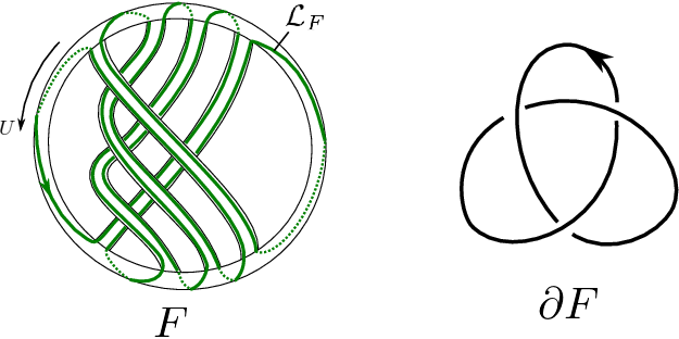
A Seifert surface $F$ is a flat plumbing basket if there are finitely many bands $B_{1},\dots,B_{n}$ and $0<\theta_{1}<\dots<\theta_{n}<2\pi$ such that $F=D_{0}\cup B_{1}\cup\dots\cup B_{n}$, each band $B_{i}$ is contained in $D_{\theta_{i}}$ and $B_{i}\cap U$ consists of two arcs. We call the subscript $i$ of $B_{i}$ the label of the band. A flat plumbing basket $F$ is a flat plumbing basket presentation of an oriented link $L$ if $\partial F$ is ambient isotopic to $L$ (for example, see Figure 2).

For a flat plumbing basket $F$, by recording the labels of the bands as one travel along $U=\partial D_{0}$, one obtain a cyclic word $W_{F}$ in $\{1,\dots,n\}$ such that each letter appears exactly twice, where $n$ is the number of the bands of $F$. We call $W_{F}$ the flat basket code for $F$.

We define the flat plumbing basket number $fpbk(L)$ of an oriented link $L$ to be the minimal number of bands to obtain a flat plumbing basket presentation of $L$ from $D_{0}$. Namely,

where $b_{1}(F)$ is the first betti number of $L$. We remark that $fpbk(L)\in 2\mathbf{Z}+|L|-1$, where $|L|$ is the number of the components of $L$, and $fpbk$ is preserved under taking mirror image.

In this section, we recall the relation between open book decompositions and contact structures. For detail, for example, see [19].

Let $M$ be an oriented closed $3$-manifold. A $1$-form $\alpha\in\Omega^{1}(M)$ is a contact form if $\alpha\wedge d\alpha$ is nowhere $0$. A $2$-dimensional distribution $\xi\subset TM$ is a contact structure if there is a contact form $\alpha$ such that $\xi=\operatorname{Ker}\alpha$. A contact structure $\xi$ on $M$ is supported by an open book decomposition $(L,\pi)$ if $\xi$ can be represented by a contact form $\alpha$ such that the binding is a transverse to $\xi$, $d\alpha$ is a volume form on every page and the orientation of binding induced by $\alpha$ agrees with the orientation of the pages.

It is known that for any open book decomposition of $M$, we can construct a contact structure on $M$ supported by the open book decomposition, by Thurston-Winkelnkemper’s construction [23]. By Giroux’s work [8], such a contact structure is unique up to contact isotopy. In particular, the trivial open book decomposition $\mathcal{O}$ of $\mathbf{S}^{3}$ supports the standard contact structure $\xi_{std}$ of $\mathbf{S}^{3}$. See Figure 3.

For a surface $\Sigma$ in $\mathbf{S}^{3}$, we consider $\xi_{std}\cap T\Sigma$. For generic $\Sigma$, this intersection is a line field except at finitely many points where $\Sigma$ is tangent to $\xi_{std}$. By integrating $\xi_{std}\cap T\Sigma$, we obtain a foliation of $\Sigma$ with singularities. Such a foliation is called the characteristic foliation of $\Sigma$ in $\xi_{std}$. In the next section, Section 3, we will construct a Legendrian link $\mathcal{L}_{F}$ from a flat plumbing basket $F$, which is isotopic to the boundary $\partial F$. Then, it is convenient to see the characteristic foliation of the boundary of a tubular neighborhood of $U$ and each fiber $D_{\theta}$ (see Figures 4 and 5).

It is known that the maximal self-linking number $\overline{sl}(L)$ and the maximal Thurston-Bennequin number $\overline{tb}(L)$ of a positive link $L$ hold the equality of the Bennequin inequality [1], that is, $\overline{sl}(L)=\overline{tb}(L)=-\chi(L)$ (for example, see [22]). In this sense, $\overline{sl}$ and $\overline{tb}$ of a positive link are large. On the other hand, as corollaries of MFW inequality and the Rasmussen bound on the maximal Thurston-Bennequin number [20, 21], we obtain

Hence, we see that the maximal self-linking number and the maximal Thurston-Bennequin number of a negative link are small. By this observation, it seems that Theorem 1.3 (or Corollary 4.4) and Theorem 1.4 (or Lemma 5.3) are effective for negative links. In particular, in Table 1, we see that $-\overline{sl}(L)-1=fpbk(L)$ for negative links $L$ with up to $9$ crossings.

For any $M>0$, there is a link $L$ such that

In fact, we can construct such a link as follows. Let $K=8_{9}$. Then, $g(8_{9})=3$ and $\max\{-\overline{tb}(8_{9}),-\overline{tb}(\overline{8_{9}})\}=5$. Let $K_{n}$ be the connected sum of $n$ copies of $8_{9}$, where we take the mirror image so that $\overline{tb}(8_{9})=-5$. It is known that $\overline{tb}(K\sharp K^{\prime})=\overline{tb}(K)+\overline{tb}(K^{\prime})+1$ for any knots $K$ and $K^{\prime}$ [24]. Hence, we obtain

By Theorem 1.2, we see that $6n+2\leq fpbk(K_{n})$. Hence, we have

Let $F$ be a flat plumbing basket. If we can draw a front (or Lagrangian) projection of $\mathcal{L}_{F}$, we may use front projections of Legendrian links to study flat plumbing baskets.

An answer to Question 6.2 is given in [12].

In this paper, we only consider the trivial open book decomposition $\mathcal{O}$ of $\mathbf{S}^{3}$. However, we can define flat plumbing baskets $F$ and the Legendrian knot $\mathcal{L}_{F}$ associated with $F$ in non-trivial open book decompositions of $\mathbf{S}^{3}$ naturally.

We improve [9, Table 1] as in Table 1, where we use Theorems 1.2, 1.3 and 1.4. In Table 1, $-\overline{tb}(K)$ means $\max\{-\overline{tb}(K),-\overline{tb}(\overline{K})\}$ and $-\overline{sl}(K)$ means $\max\{-\overline{sl}(K),-\overline{sl}(\overline{K})\}$. We refer to [18, Proposition 1.6] for $\overline{sl}(K)$ and [2] for $\overline{tb}(K)$. Note that $fpbk(K)\in 2\mathbf{Z}$ for a knot $K$.

In this table, the asterisks ^∗ are improved points of [9, Table 1]. The double asterisks ^∗∗ are given by [3] and Mikami Hirasawa. In fact, Mikami Hirasawa taught the author that a flat basket code for $8_{1}$ is $(1,2,4,5,3,6,1,4,6,2,5,3)$ and a flat basket code for $9_{44}$ is $(1,2,5,6,1,4,3,5,6,2,4,3)$. The daggers ^† mean that Theorem 1.3 or  1.4 detects $fpbk(K)$.

For example, $8_{15}$ has a flat plumbing basket presentation $F$ with $b_{1}(F)=10$. On the other hand, it is known that $\max\{-\overline{sl}(8_{15}),-\overline{sl}(\overline{8_{15}})\}=11$ (see [18, Proposition 1.6]). Hence, by Theorem 1.3, we have $fpbk(8_{15})=10$.

For another example, the knot $9_{45}$ has a flat plumbing basket presentation $F$ with $b_{1}(F)=8$. On the other hand, it is known that $\max\{-\overline{tb}(9_{45}),-\overline{tb}(\overline{9_{45}})\}=10$ (for example, see [2]). Moreover, $9_{45}$ is a non-torus knot. Hence, by Theorem 1.4, we have $10+3=13\leq 2fpbk(9_{45})\leq 16$. Since $fpbk(9_{45})\in 2\mathbf{Z}$, we have $fpbk(9_{45})=8$.

Note that $fpbk$ is subadditive under connected sum of knots. However, in general, it is not additive. For example, Hirose-Nakashima [9, Remark 1.4(b)] proved that $fpbk(3_{1})=fpbk(\overline{3_{1}})=4$ but $fpbk(3_{1}\sharp\overline{3_{1}})=6$. Nao Kobayashi (Imoto) proved that $fpbk(6_{1})=fpbk(\overline{6_{1}})=6$ but $fpbk(6_{1}\sharp\overline{6_{1}})=8$ in [15, Proposition 5.4].

References

- [1] D. Bennequin, Entrelacements et équations de Pfaff, Third Schnepfenried geometry conference, Vol. 1 (Schnepfenried, 1982), Astérisque, vol. 107, Soc. Math. France, Paris, 1983, pp. 87–161. MR 753131 (86e:58070)
- [2] J. C. Cha and C. Livingston, KnotInfo, http://www.indiana.edu/%7eknotinfo/.
- [3] Y. H. Choi, Y. K. Chung, and D. Kim, The complete list of prime knots whose flat plumbing basket numbers are 6 or less, J. Knot Theory Ramifications 24 (2015), no. 7, 1550042, 13.
- [4] J. B. Etnyre, L. L. Ng, and V. Vértesi, Legendrian and transverse twist knots, J. Eur. Math. Soc. (JEMS) 15 (2013), no. 3, 969–995. MR 3085098
- [5] J. Franks and R. F. Williams, Braids and the Jones polynomial, Trans. Amer. Math. Soc. 303 (1987), no. 1, 97–108. MR 896009 (88k:57006)
- [6] R. Furihata, M. Hirasawa, and T. Kobayashi, Seifert surfaces in open books, and a new coding algorithm for links, Bull. Lond. Math. Soc. 40 (2008), no. 3, 405–414. MR 2418796
- [7] H. Geiges, An introduction to contact topology, Cambridge Studies in Advanced Mathematics, vol. 109, Cambridge University Press, Cambridge, 2008. MR 2397738
- [8] E. Giroux, Géométrie de contact: de la dimension trois vers les dimensions supérieures, Proceedings of the International Congress of Mathematicians, Vol. II (Beijing, 2002), Higher Ed. Press, Beijing, 2002, pp. 405–414. MR 1957051
- [9] S. Hirose and Y. Nakashima, Seifert surfaces in open books, and pass moves on links, J. Knot Theory Ramifications 23 (2014), no. 4, 1450021, 12. MR 3218929
- [10] K. Honda, On the classification of tight contact structures. I, Geom. Topol. 4 (2000), 309–368. MR 1786111
- [11] N. Imoto, On an estimation of flat plumbing basket number of knots, JP J. Geom. Topol. 18 (2015), no. 1, 65–84. MR 3445276
- [12] T. Ito and K. Tagami, Flat plumbing basket and contact structure, arXiv:1710.11363.
- [13] D. Kim, An alternating labeling on a spanning tree of seifert graphs and applications in knot theory, arXiv:1108.1455.
- [14] D. Kim, Y. S. Kwon, and J. Lee, Banded surfaces, banded links, band indices and genera of links, J. Knot Theory Ramifications 22 (2013), no. 7, 1350035, 18. MR 3084753
- [15] N. Kobayashi (Imoto), Basket diagram and its application to flat plumbing basket number of links, 2017, Thesis (Ph.D.)–Nara Women’s University.
- [16] H. R. Morton, Seifert circles and knot polynomials, Math. Proc. Cambridge Philos. Soc. 99 (1986), no. 1, 107–109. MR 809504 (87c:57006)
- [17] L. Ng, A Legendrian Thurston-Bennequin bound from Khovanov homology, Algebr. Geom. Topol. 5 (2005), 1637–1653. MR 2186113
- [18] by same author, On arc index and maximal Thurston-Bennequin number, J. Knot Theory Ramifications 21 (2012), no. 4, 1250031, 11. MR 2890458
- [19] B. Ozbagci and A. I. Stipsicz, Surgery on contact 3-manifolds and Stein surfaces, Bolyai Society Mathematical Studies, vol. 13, Springer-Verlag, Berlin; János Bolyai Mathematical Society, Budapest, 2004. MR 2114165
- [20] O. Plamenevskaya, Transverse knots and Khovanov homology, Math. Res. Lett. 13 (2006), no. 4, 571–586. MR 2250492 (2007d:57043)
- [21] A. N. Shumakovitch, Rasmussen invariant, slice-Bennequin inequality, and sliceness of knots, J. Knot Theory Ramifications 16 (2007), no. 10, 1403–1412. MR 2384833 (2008m:57034)
- [22] T. Tanaka, Maximal Bennequin numbers and Kauffman polynomials of positive links, Proc. Amer. Math. Soc. 127 (1999), no. 11, 3427–3432. MR 1616601
- [23] W. Thurston and H. Winkelnkemper, On the existence of contact forms, Proc. Amer. Math. Soc. 52 (1975), 345–347. MR 0375366
- [24] I. Torisu, On the additivity of the Thurston-Bennequin invariant of Legendrian knots, Pacific J. Math. 210 (2003), no. 2, 359–365. MR 1988540