Estimation of the Hurst Exponent
Using Trimean Estimators on
Nondecimated Wavelet Coefficients
Abstract
Hurst exponent is an important feature summarizing the noisy high-frequency data when the inherent scaling pattern cannot be described by standard statistical models. In this paper, we study the robust estimation of Hurst exponent based on non-decimated wavelet transforms (NDWT). The robustness is achieved by applying a general trimean estimator on non-decimated wavelet coefficients of the transformed data. The general trimean estimator is derived as a weighted average of the distribution’s median and quantiles, combining the median’s emphasis on central values with the quantiles’ attention to the extremes. The properties of the proposed Hurst exponent estimators are studied both theoretically and numerically. Compared with other standard wavelet-based methods (Veitch Abry (VA) method, Soltani, Simard, Boichu (SSB) method, median based estimators MEDL and MEDLA), our methods reduce the variance of the estimators and increase the prediction precision in most cases. The proposed methods are applied to a data set in high frequency pupillary response behavior (PRB) with the goal to classify individuals according to a degree of their visual impairment.
Index Terms:
Hurst exponent, Time series, High-frequency data, Robust estimation, Non-decimated wavelet transforms, General trimean estimator, Median, Quantiles.I Introduction
High-frequency, time series data from various sources often possess hidden patterns that reveal the effects of underlying functional differences, but such patterns cannot be explained by basic descriptive statistics, traditional statistical models, or global trends. For example, the high-frequency pupillary response behavior (PRB) data collected during human-computer interaction capture the changes in pupil diameter in response to simple or complex stimuli. Researchers found that there may be underlying unique patterns hidden within complex PRB data, and these patterns reveal the intrinsic individual differences in cognitive, sensory and motor functions [1]. Yet, such patterns cannot be explained by the traditional statistical summaries of the PRB data, for the magnitude of the diameter depends on ambient light, not on the inherent eye function [2]. When the intrinsic individual functional differences cannot be described by basic statistics and trends in the noisy high-frequency data, the Hurst exponent might be an optional measure of patients’ characterization.
The Hurst exponent quantifies the long memory as well as regularity, self-similarity, and scaling in a time series. Among models having been proposed for analyzing the self-similar phenomena, arguably the most popular is the fractional Brownian motion (fBm) first described by Kolmogorov [3] and formalized by Mandelbrot and Van Ness [4]. Its importance is due to the fact that fBm is the unique Gaussian process with stationary increments that is self-similar. Recall that a stochastic process is self-similar with Hurst exponent if, for any , . Here the notation means the equality in all finite-dimensional distributions. Hurst exponent describes the rate at which autocorrelations decrease as the lag between two realizations in a time series increases.
A value in the range 0-0.5 indicates a zig-zagging intermittent time series with long-term switching between high and low values in adjacent pairs. A value in the range 0.5 to 1 indicates a time series with long-term positive autocorrelations, which preserves trends on a longer time horizon and gives a time series more regular appearance.
Multiresolution analysis is one of the many methods to estimate the Hurst exponent . An overview can be found in [5, 6, 7]. If processes possess a stochastic structure, i.e., Gaussianity and stationary increments, becomes a parameter in a well-defined statistical model and can be estimated after taking the of the quantity , where ’s are the wavelet coefficients at level . In fact, several estimation methods of based on wavelets analysis exist. Veitch and Abry [5] suggest the estimation of by weighted least square regression using the level-wise since the variance of depends on and the level . In addition, the authors correct for the bias caused by the order of taking the logarithm and the average in . Soltani et al [8] defined a mid-energy as , and showed that the level-wise averages of are asymptotically normal and more stable, which is used to estimate parameter by regression. The estimators in Soltani et al [8] consistently outperform the estimators in Veitch and Abry [5]. Shen et al [9] shows that the method of Soltani et al [8] yields more accurate estimators since it takes the logarithm of the mid-energy and then averages. Kang and Vidakovic [2] proposed MEDL and MEDLA methods based on non-decimated wavelets to estimate . MEDL estimates by regressing the medians of on level , while MEDLA uses the level-wise medians of to estimate , where and are properly selected locations at level to guarantee the independence assumption. Both MEDL and MEDLA use the median of the derived distribution instead of the mean, because the medians are more robust to potential outliers that can occur when logarithmic transform of a squared wavelet coefficient is taken and the magnitude of coefficient is close to zero. Although median is outlier-resistant, it can behave unexpectedly as a result of its non-smooth character. The fact that the median is not “universally the best outlier-resistant estimator” provides a practical motivation for examining alternatives that are intermediate in behavior between the very smooth but outlier-sensitive mean and the very outlier-insensitive but non-smooth median. In this article, the general trimean estimator is derived as a weighted average of the distribution’s median and two quantiles symmetric about the median, combining the median’s emphasis on center values with the quantiles’ attention to the tails. Tukey’s trimean estimator [10, 11] and Gastwirth estimator [12, 13, 14] turn out to be two special cases under the general framework. We will use the general trimean estimators of the level-wise derived distributions to estimate . In this paper, we are concerned with the robust estimation of Hurst exponent in one-dimensional setting, however, the methodology can be readily extended to a multidimensional case.
The rest of the paper consists of five additional sections and an appendix. Section 2 introduces the general trimean estimators and discusses two special estimators following that general framework; Section 3 describes estimation of Hurst exponent using the general trimean estimators, presents distributional results on which the proposed methods are based, and derives optimal weights that minimize the variances of the estimators. Section 4 provides the simulation results and compares the performance of the proposed methods to other standardly used, wavelet-based methods. The proposed methods are illustrated using the real PRB data in Section 5. The paper is concluded with a summary and discussion in Section 6.
II General Trimean Estimators
Let be i.i.d. continuous random variables with pdf and cdf . Let , and let denote the th quantile of , so that If is monotone, the th quantile is simply defined as .
Let denote a sample th quantile. Here denotes the greatest integer that is less than or equal to . The general trimean estimator is defined as a weighted average of the distribution’s median and its two quantiles and , for :
| (1) |
The weights for the two quantiles are the same for and , and . This is equivalent to the weighted sum of the median and the average of and with weights and :
This general trimean estimator turns out to be more robust then mean but smoother than the median. To derive the asymptotic distribution of this general trimean estimator, the asymptotic joint distribution of sample quantiles is shown in Lemma 1; detailed proof can be found in [15].
Lemma 1.
Consider sample quantiles, , where . If for any , is satisfied, then the asymptotic joint distribution of is:
where
and
| (2) |
From Lemma 1, the asymptotic distribution of general trimean estimator will be normal as a linear combination of the components of the asymptotic multivariate normal distribution. The general trimean estimator itself may be defined in terms of order statistics as
where
It can be easily verified that for . If we denote the population quantiles, the asymptotic distribution of is
where and follows equation (2) for . Therefore
with the theoretical expectation and variance being
| (3) |
and
| (4) |
II-A Tukey’s Trimean Estimator
Tukey’s trimean estimator is a special case of the general trimean estimators, with and in equation (1). To compute this estimator, we first sort the data in ascending order. Next, we take the values that are one-forth of the way up this sequence (the first quartile), half way up the sequence (i.e., the median), and three-fourths of the way up the sequence (the thirt quartile). Given these three values, we then form the weighted average, giving the central (median) value a weight of and the two quartiles each a weight of . If we denote the Tukey’s trimean estimator as then
The Tukey’s trimean estimator may be expressed more compactly as
where
It can be easily verified that for . If we denote the corresponding theoretical quantiles, the asymptotic distribution of is
where is the covariance matrix of the asymptotic multivariate normal distribution, and follows equation (2) with .
II-B Gastwirth Estimator
As the Tukey’s estimator, the Gastwirth estimator is another special case of the general trimean estimators, with and in equation (1). If we denote this estimator as , then
The Gastwirth estimator can be written as
where
As in Tukey’s case, if we denote as the theoretical quantiles, since for , the asymptotic distribution of is
where , and follows equation (2) with .
III Methods
Our proposal for robust estimation of Hurst exponent is based on non-decimated wavelet transforms (NDWT). Details of NDWT can be found in [16, 17, 18]. The comparison of NDWT and standard orthogonal discrete wavelet transforms (DWT) has been discussed by Kang and Vidakovic [2]. NDWT has several advantages when employed for Hurst exponent estimation: 1) Input signals and images of arbitrary size can be processed due to the absence of decimation; 2) as a redundant transform, the NDWT increases the accuracy of the scaling estimation; 3) least square regression can be fitted to estimate instead of weighted least square regression since the variances of the level-wise derived distributions based on logged NDWT coefficients do not depend on level; 4) local scaling can be assessed due to the time-invariance property. Of course, as we will discuss later, the dependence of coefficients in NDWT is much more pronounced than in the case of DWT.
In -level decomposition of a fBm of size , a NDWT yields wavelet coefficients, with each level coefficients. At each level , we generate mid-energies as
| (5) |
The distributions of the and are derived under the assumption that and are independent. Then we apply the general trimean estimators of the level-wise derived distributions to estimate parameter . Note that for fixed , the generated mid-energies and are not independent but their autocorrelations decay exponentially, consequently, they posses only the short memory. At each level , we sample every points from and to form groups, and assume that the points of and within each subgroup are independent, respectively. The general trimean estimators are then applied on each of the groups. Note that must be divisible by .
| Group 1: and Group 2: and ⋮ Group M: and |
III-A General Trimean of the Mid-energy (GTME) Method
For the general trimean of the mid-energy (GTME) method, we derive the relationship between the general trimean estimator of each mid-energy groups from decomposition level The GTME method is described in the following theorem:
Theorem III.1.
Let be the general trimean estimator based on
, where for and is the th group of mid-energies at level in a -level NDWT of a fBm of size with Hurst exponent . Then, the asymptotic distribution of is normal,
| (6) |
where
In the previous, is the standard deviation of wavelet coefficients from level 0. The Hurst exponent can be estimated as
| (7) |
where is the average of regression slopes in the least square linear regression on pairs over the groups, .
The proof of Theorem III.1 is deferred to the appendix.
To find the optimal and minimizing the asymptotic variance of , we take partial derivatives of with respect to and and set them to 0. The optimal and can be obtained by solving
| (8) | ||||
Since , and , we get the unique solution and . The Hessian matrix of is
Since and the determinant is when and , the above Hessian matrix is positive definite. Therefore, and provide the global minima of , minimizing also the asymptotic variance of . In comparing these optimal and with and from the Gastwirth estimator, curiously, we find that the optimal general trimean estimator is very close to the Gastwirth estimator.
III-B General Trimean of the Logarithm of Mid-energy (GTLME) Method
Previously discussed the GTME method calculates the general trimean estimator of the mid-energy first and then takes the logarithm. In this section, we will calculate the general trimean estimator of the logged mid-energies at each subgroup from level . The following theorem describes the general trimean of the logarithm of mid-energy, the GTLME method.
Theorem III.2.
Let be the general trimean estimator based on
, where is the th group of logged mid-energies” at level in a -level NDWT of a fBm of size with Hurst exponent , and . Then, the asymptotic distribution of is normal,
| (9) |
where
and
and are two functions of ,
and is the variance of wavelet coefficients from level 0. The Hurst exponent can be estimated as
| (10) |
where is the average of regression slopes in the least square linear regressions on pairs over the groups, .
The proof of Theorem III.2 is provided in the appendix. Similarly, as for the GTME, the optimal and which minimize the asymptotic variance of can be obtained by solving
| (11) |
From the first equation in (11) it can be derived that
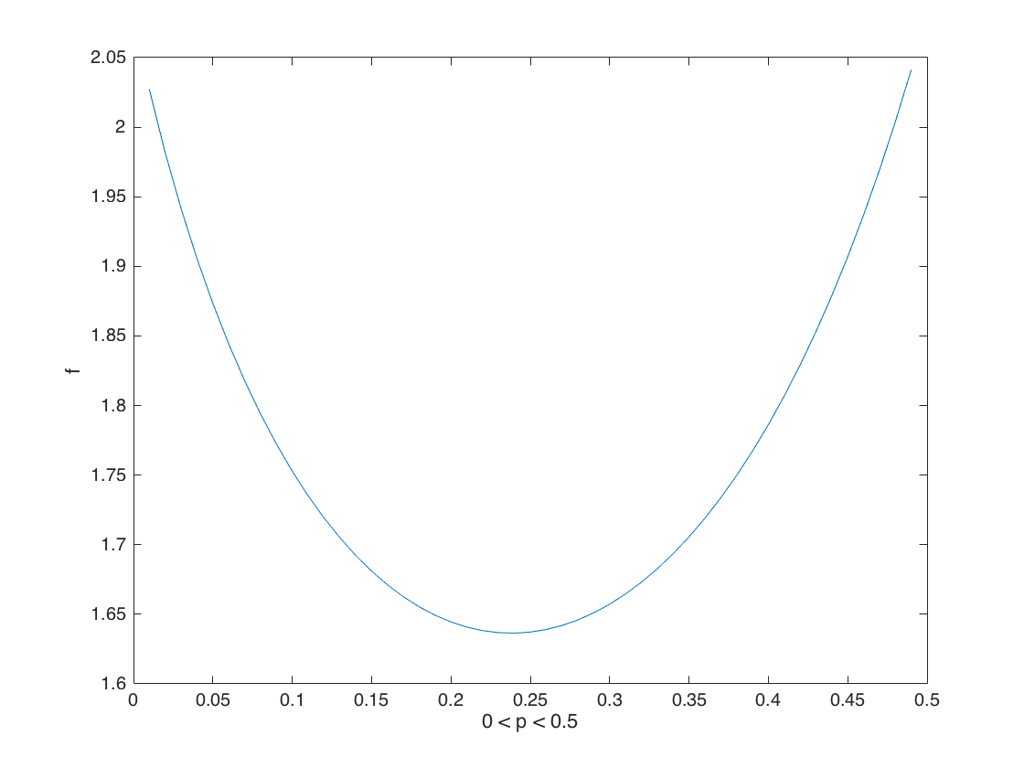
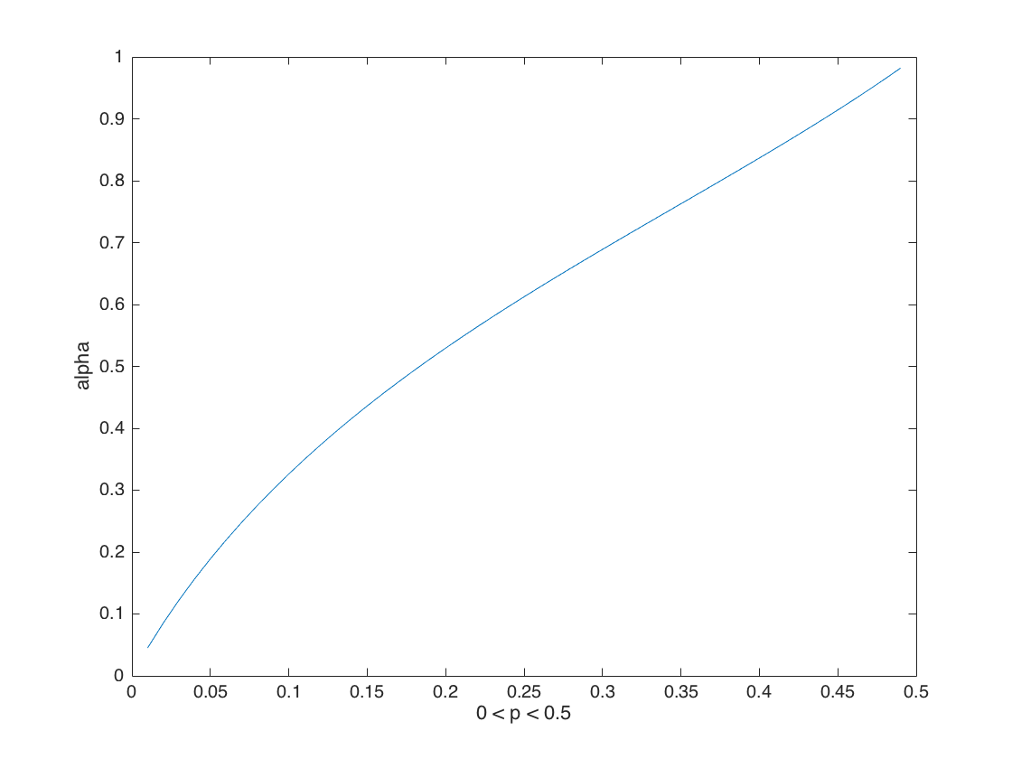
The second equation in (11) cannot be simplified to a finite form. As an illustration, we plot the with ranging from 0 to 0.5 and being a function of . The plot of against is also shown in Figure 1. Numerical calculation gives and . These optimal parameters are close to and in the Tukey’s trimean estimator, but put some more weight on the median.
III-C Special Cases: Tukey’s Trimean and Gastwirth Estimators
The Tukey’s trimean of the mid-energy (TTME) method and Gastwirth of the mid-energy (GME) method are described in the following Lemma.
Lemma 2.
Let and be the Tukey’s trimean and Gastwirth estimators based on defined in the Theorem III.1. Then the asymptotic distributions of and are normal:
| (12) |
| (13) |
where and are constants independent of , , and is the variance of wavelet coefficients from level 0. The Hurst exponent can be estimated as
| (14) |
where and are the averages of regression slopes in the least square linear regression on pairs and pairs over the groups, respectively ().
The following Lemma describes the Tukey’s trimean (TTLME) and Gastwirth (GLME) of the logarithm of mid-energy method.
Lemma 3.
Let and be the Tukey’s trimean estimator and Gastwirth estimator based on defined in the Theorem III.2. The asymptotic distributions of and are normal,
| (15) |
| (16) |
where ,, and are constants independent of level . The Hurst exponent can be estimated as
| (17) |
where and are the averages of regression slopes in the least square linear regression on pairs and pairs ,, over the groups.
IV Simulation
We simulate fractional Brownian motion (fBm) signals of sizes , and with Hurst exponent , respectively. NDWT of depth using Pollen wavelets with angles (Daubechies 2), , , and (Haar) are performed on each simulated signal to obtain wavelet coefficients. Pollen generates a family possessing continuum many wavelet bases of various degrees of regularity [19]. Special cases of Pollen’s representation for and give Daubechies 2 filter and Haar filter, respectively. Figure 2 depicts scaling and wavelet functions for .
The proposed methods (with 6 variations) are applied on the NDWT coefficients to estimate Hurst exponent . Coefficients on each level are divided into eight groups () for all proposed methods, and we use wavelet coefficients from levels 4 to 10 for the least square linear regression. The estimation performance of the proposed methods are compared to four other existing methods: Veitch Abry (VA) method, Soltani, Simard, Boichu (SSB) method, MEDL method, and MEDLA method. The GTME and GTLME methods are based on the optimal parameters to minimize the variances. Estimation performances are compared in terms of mean, variance, and mean square error (MSE) based on 300 repetitions for each case.
The proposed methods preform the best using Haar wavelet (Pollen wavelets with angle ), and the simulation results are shown in Table I to Table III for fBm of sizes , and , respectively. Similar results are obtained for other wavelets. For each (corresponding to each row in the table), the smallest variances and MSEs are highlighted in bold. From simulations results, at least one of our 6 variations outperforms MEDL and MEDLA for all and fBm of all three sizes. Compared with VA and SSB methods, our methods yield significantly smaller variances and MSEs when for fBm of all three sizes. When , our methods are still comparable to VA and SSB. Although the performances of our 6 variations are very similar regarding to variances and MSEs, the TTME method based on Tukey’s trimean estimator of the mid-energy has the best performance among all of them. As expected, the variances of GTME based on the optimal parameters are smaller than or equal to those of GME and TTME methods in most cases, and similarly, in most cases the optimized GTLME method is superior to other logged mid-energy methods TTLME and GLME with respect to variances. However, this superiority is not significant, since the variances of all six proposed methods are close to each other.

| Methods | ||||||||||
| VA | SSB | MEDL | MEDLA | TTME | GME | TTLME | GLME | GTME | GTLME | |
| 0.3 | 0.2429 | 0.2429 | 0.2368 | 0.2365 | 0.2397 | 0.2393 | 0.2393 | 0.2390 | 0.2395 | 0.2396 |
| 0.5 | 0.4482 | 0.4944 | 0.4800 | 0.4821 | 0.4893 | 0.4870 | 0.4872 | 0.4861 | 0.4882 | 0.4876 |
| 0.7 | 0.5209 | 0.7232 | 0.6996 | 0.7002 | 0.7094 | 0.7072 | 0.7067 | 0.7058 | 0.7085 | 0.7071 |
| 0.8 | 0.5171 | 0.8304 | 0.7999 | 0.7991 | 0.8050 | 0.8020 | 0.8031 | 0.8008 | 0.8037 | 0.8044 |
| 0.9 | 0.4976 | 0.9410 | 0.9020 | 0.8951 | 0.9016 | 0.9004 | 0.9024 | 0.9009 | 0.9012 | 0.9032 |
| Variances | ||||||||||
| 0.3 | 0.0024 | 0.0024 | 0.0025 | 0.0022 | 0.0020 | 0.0021 | 0.0022 | 0.0022 | 0.0021 | 0.0022 |
| 0.5 | 0.0018 | 0.0034 | 0.0035 | 0.0030 | 0.0030 | 0.0031 | 0.0031 | 0.0031 | 0.0030 | 0.0030 |
| 0.7 | 0.0048 | 0.0055 | 0.0049 | 0.0038 | 0.0036 | 0.0036 | 0.0038 | 0.0037 | 0.0036 | 0.0038 |
| 0.8 | 0.0067 | 0.0071 | 0.0061 | 0.0044 | 0.0041 | 0.0044 | 0.0047 | 0.0047 | 0.0042 | 0.0047 |
| 0.9 | 0.0064 | 0.0085 | 0.0066 | 0.0047 | 0.0041 | 0.0043 | 0.0047 | 0.0046 | 0.0042 | 0.0047 |
| MSEs | ||||||||||
| 0.3 | 0.0057 | 0.0056 | 0.0065 | 0.0062 | 0.0056 | 0.0058 | 0.0059 | 0.0059 | 0.0057 | 0.0058 |
| 0.5 | 0.0044 | 0.0034 | 0.0038 | 0.0034 | 0.0031 | 0.0032 | 0.0032 | 0.0033 | 0.0031 | 0.0032 |
| 0.7 | 0.0368 | 0.0060 | 0.0049 | 0.0038 | 0.0037 | 0.0036 | 0.0038 | 0.0037 | 0.0037 | 0.0039 |
| 0.8 | 0.0867 | 0.0080 | 0.0061 | 0.0044 | 0.0042 | 0.0044 | 0.0047 | 0.0047 | 0.0042 | 0.0047 |
| 0.9 | 0.1683 | 0.0101 | 0.0066 | 0.0047 | 0.0041 | 0.0043 | 0.0047 | 0.0046 | 0.0042 | 0.0047 |
| Methods | ||||||||||
| VA | SSB | MEDL | MEDLA | TTME | GME | TTLME | GLME | GTME | GTLME | |
| 0.3 | 0.2448 | 0.2420 | 0.2385 | 0.2382 | 0.2393 | 0.2389 | 0.2392 | 0.2390 | 0.2392 | 0.2394 |
| 0.5 | 0.4548 | 0.4822 | 0.4721 | 0.4725 | 0.4755 | 0.4745 | 0.4743 | 0.4740 | 0.4749 | 0.4744 |
| 0.7 | 0.5216 | 0.7125 | 0.6917 | 0.6931 | 0.6977 | 0.6963 | 0.6959 | 0.6954 | 0.6969 | 0.6963 |
| 0.8 | 0.5224 | 0.8201 | 0.7937 | 0.7933 | 0.7986 | 0.7972 | 0.7979 | 0.7970 | 0.7979 | 0.7985 |
| 0.9 | 0.5028 | 0.9301 | 0.8988 | 0.8922 | 0.8958 | 0.8957 | 0.8976 | 0.8965 | 0.8958 | 0.8982 |
| Variances | ||||||||||
| 0.3 | 0.0013 | 0.0011 | 0.0011 | 0.0010 | 0.0010 | 0.0010 | 0.0010 | 0.0010 | 0.0010 | 0.0010 |
| 0.5 | 0.0006 | 0.0013 | 0.0015 | 0.0011 | 0.0010 | 0.0011 | 0.0011 | 0.0012 | 0.0011 | 0.0011 |
| 0.7 | 0.0041 | 0.0022 | 0.0022 | 0.0016 | 0.0015 | 0.0015 | 0.0016 | 0.0016 | 0.0015 | 0.0016 |
| 0.8 | 0.0071 | 0.0039 | 0.0035 | 0.0026 | 0.0023 | 0.0025 | 0.0026 | 0.0026 | 0.0024 | 0.0026 |
| 0.9 | 0.0065 | 0.0053 | 0.0046 | 0.0032 | 0.0027 | 0.0029 | 0.0032 | 0.0032 | 0.0028 | 0.0032 |
| MSEs | ||||||||||
| 0.3 | 0.0044 | 0.0044 | 0.0049 | 0.0048 | 0.0046 | 0.0047 | 0.0047 | 0.0047 | 0.0046 | 0.0046 |
| 0.5 | 0.0027 | 0.0016 | 0.0023 | 0.0019 | 0.0016 | 0.0018 | 0.0018 | 0.0018 | 0.0017 | 0.0018 |
| 0.7 | 0.0359 | 0.0024 | 0.0023 | 0.0016 | 0.0015 | 0.0016 | 0.0016 | 0.0017 | 0.0015 | 0.0016 |
| 0.8 | 0.0841 | 0.0042 | 0.0035 | 0.0027 | 0.0023 | 0.0025 | 0.0026 | 0.0026 | 0.0024 | 0.0026 |
| 0.9 | 0.1642 | 0.0062 | 0.0046 | 0.0033 | 0.0027 | 0.0029 | 0.0032 | 0.0032 | 0.0028 | 0.0032 |
| Methods | ||||||||||
| VA | SSB | MEDL | MEDLA | TTME | GME | TTLME | GLME | GTME | GTLME | |
| 0.3 | 0.2427 | 0.2364 | 0.2337 | 0.2339 | 0.2342 | 0.2339 | 0.2341 | 0.2339 | 0.2341 | 0.2343 |
| 0.5 | 0.4585 | 0.4759 | 0.4672 | 0.4679 | 0.4701 | 0.4691 | 0.4693 | 0.4686 | 0.4695 | 0.4695 |
| 0.7 | 0.5228 | 0.7002 | 0.6843 | 0.6857 | 0.6890 | 0.6882 | 0.6879 | 0.6877 | 0.6885 | 0.6879 |
| 0.8 | 0.5124 | 0.8104 | 0.7925 | 0.7907 | 0.7932 | 0.7928 | 0.7930 | 0.7928 | 0.7929 | 0.7932 |
| 0.9 | 0.4935 | 0.9190 | 0.8976 | 0.8928 | 0.8932 | 0.8935 | 0.8951 | 0.8945 | 0.8932 | 0.8954 |
| Variances | ||||||||||
| 0.3 | 0.0009 | 0.0006 | 0.0007 | 0.0006 | 0.0006 | 0.0006 | 0.0006 | 0.0006 | 0.0006 | 0.0006 |
| 0.5 | 0.0004 | 0.0007 | 0.0008 | 0.0006 | 0.0005 | 0.0006 | 0.0006 | 0.0006 | 0.0006 | 0.0006 |
| 0.7 | 0.0046 | 0.0013 | 0.0012 | 0.0010 | 0.0009 | 0.0010 | 0.0010 | 0.0010 | 0.0010 | 0.0010 |
| 0.8 | 0.0060 | 0.0019 | 0.0018 | 0.0014 | 0.0013 | 0.0014 | 0.0014 | 0.0015 | 0.0013 | 0.0014 |
| 0.9 | 0.0049 | 0.0031 | 0.0028 | 0.0021 | 0.0019 | 0.0020 | 0.0021 | 0.0021 | 0.0019 | 0.0021 |
| MSEs | ||||||||||
| 0.3 | 0.0042 | 0.0046 | 0.0051 | 0.0050 | 0.0049 | 0.0050 | 0.0049 | 0.0050 | 0.0049 | 0.0049 |
| 0.5 | 0.0021 | 0.0012 | 0.0019 | 0.0016 | 0.0014 | 0.0015 | 0.0016 | 0.0016 | 0.0015 | 0.0015 |
| 0.7 | 0.0360 | 0.0013 | 0.0015 | 0.0012 | 0.0011 | 0.0011 | 0.0012 | 0.0012 | 0.0011 | 0.0012 |
| 0.8 | 0.0887 | 0.0020 | 0.0019 | 0.0015 | 0.0013 | 0.0014 | 0.0015 | 0.0015 | 0.0014 | 0.0015 |
| 0.9 | 0.1702 | 0.0035 | 0.0028 | 0.0021 | 0.0019 | 0.0020 | 0.0021 | 0.0021 | 0.0019 | 0.0021 |
V Application
In this section, we apply the proposed methodology to high frequency measurements in pupillary response behavior (PRB). PRB refers to changes in pupil diameter in response to simple or complex stimuli. Participants in this study included 24 older adults, solicited from the patient pool of the Bascom Palmer Eye Institute of the University of Miami School of Medicine. Participants were selected on the basis of having either no ocular disease or only Age-related Macular Degeneration (AMD), as assessed by patient history and clinical testing. Participants were selected based on the diagnosis of AMD and their best eye near distance (40 cm) visual acuity.
Participants were assigned to 3 groups ( one control group and 2 experimental groups). The control group is a set of individuals with healthy, unaffected vision and no evidence of any ocular disease or trauma. Individuals in 2 experimental groups had varying visual acuity and were diagnosed with AMD. The number of participants is 6 in control group, 12 in group I, and 6 in group II. The data analysis process consists of first cleaning the data by removing the blink and equipment artifacts and then segmenting the data stream for each participant into equal length pieces of 2048 observations. The number of 2048 length data sets that were extracted from the collective data sets of the individuals within each group are shown in Table IV.
Traditional statistical methods have not been successfully used for examining the PRB of older adults or individuals with visual impairments. Researchers have utilized simple statistical methods for analyzing PRB, for example, comparing the relative mean or variance of pupil size deviation in response to stimuli; some sophisticated techniques have also been utilized, like power, frequency and spectral analysis using mathematical tools. But most of them failed to characterize the underlying patterns within time series PRB data. Wavelet analysis to estimate the Hurst exponent of the high-frequency, time series physiological data is a useful tool for detecting these hidden patterns and differentiating individuals based on these unique patterns in their physiological behavior.
Table V provides descriptive statistics of the estimated Hurst exponent in each group using our proposed methods and four standard methods to compare with. As can be seen, there are clear monotonic trends for across the participant groups. The control group exhibited the smallest value for , followed by group I and group II, and those monotonic trends are presented in both the mean and median values. In fact, signals with smaller Hurst exponent tend to be more disordered and unsystematic, therefore the monotonic trends indicating that individuals with higher severity of visual impairment have less disordered pupil diameter signals. Similar results for original data without being pre-processed are shown in Table VI. No monotonic trends of across groups have been observed in original data, indicating the blinks indeed add noise to the data.
Like in many human-subject studies, the limited number of participants is a major disadvantage, but in PRB data set, each subject has enough measurements to segment into multiple pieces with a length of 2048 observations. This induces dependence between the runs, and hierarchical models accommodating for the subject induced dependence are needed. If we denote to be the group index where the piece of observations is from, with for control group, for group I, for group II, and as the number of pieces generated from subject (j=1,2,..,24), the estimated Hurst exponent for the th piece of subject nested in group can be expressed in the following model:
| (18) |
where is the overall mean, is the effect for th group, is the effect for th participant within th group, and is the random error. The objective is to classify the groups based on the estimated Hurst exponent for a given pupil diameter data. In avoid of dependency between data sets due to subject effects, the estimated is first subtracted from , and multinomial logistic regression model is fitted on the data . To test the model performance, we randomly choose of the data points to form a training set, and the remaining forms the testing set. Model is developed on the training set and applied on the testing set; misclassification rate is reported in Table VII.
| Group | N | Visual Acuity | AMD | Number of preprocessed data sets |
|---|---|---|---|---|
| Control | 6 | 20/20-20/40 | No | 49 |
| I | 12 | 20/20-20/100 | Yes | 184 |
| II | 6 | 20/100 | Yes | 170 |
- •
Note. N represents the number of individuals in the group; Visual Acuity represents the range of Snellen acuity scores for the individuals in the given group, AMD represents whether the individuals were diagnosed with age-related macular degeneration or not, and Number of cleaned data sets shows the number of 2048 length data sets extracted from individuals within each group.
| Methods | ||||||||||
| Group | Veitch and Abry | Soltani | MEDL | MEDLA | TTME | GME | TTLME | GLME | GTME | GTLME |
| Mean of | ||||||||||
| Control | 0.1495 | 0.4103 | 0.2741 | 0.2501 | 0.2416 | 0.2505 | 0.2537 | 0.2559 | 0.2467 | 0.2530 |
| I | 0.1855 | 0.4210 | 0.2733 | 0.2727 | 0.2638 | 0.2686 | 0.2716 | 0.2738 | 0.2666 | 0.2705 |
| II | 0.1682 | 0.5464 | 0.3597 | 0.3202 | 0.2984 | 0.3116 | 0.3257 | 0.3231 | 0.3057 | 0.3286 |
| Median of | ||||||||||
| Control | 0.1474 | 0.4088 | 0.2869 | 0.2596 | 0.2535 | 0.2609 | 0.2625 | 0.2683 | 0.2577 | 0.2615 |
| I | 0.2073 | 0.4331 | 0.3033 | 0.2951 | 0.2938 | 0.2990 | 0.3054 | 0.3038 | 0.2976 | 0.3042 |
| II | 0.1814 | 0.5436 | 0.3514 | 0.3240 | 0.2973 | 0.3127 | 0.3261 | 0.3313 | 0.3058 | 0.3254 |
| Variance of | ||||||||||
| Control | 0.0084 | 0.0195 | 0.0088 | 0.0086 | 0.0091 | 0.0094 | 0.0092 | 0.0094 | 0.0095 | 0.0092 |
| I | 0.0120 | 0.0421 | 0.0213 | 0.0206 | 0.0191 | 0.0196 | 0.0200 | 0.0204 | 0.0194 | 0.0198 |
| II | 0.0114 | 0.0373 | 0.0428 | 0.0066 | 0.0061 | 0.0060 | 0.0087 | 0.0065 | 0.0060 | 0.0102 |
| Methods | ||||||||||
| Group | Veitch and Abry | Soltani | MEDL | MEDLA | TTME | GME | TTLME | GLME | GTME | GTLME |
| Mean of | ||||||||||
| Control | 0.1892 | 0.4627 | 0.3582 | 0.3497 | 0.3394 | 0.3498 | 0.3473 | 0.3498 | 0.3459 | 0.3446 |
| I | 0.1812 | 0.4272 | 0.2860 | 0.2918 | 0.2858 | 0.2900 | 0.2900 | 0.2923 | 0.2891 | 0.2888 |
| II | 0.1565 | 0.5510 | 0.3672 | 0.3295 | 0.3113 | 0.3262 | 0.3373 | 0.3360 | 0.3201 | 0.3416 |
| Median of | ||||||||||
| Control | 0.2144 | 0.5194 | 0.3502 | 0.3574 | 0.3464 | 0.3559 | 0.3513 | 0.3542 | 0.3510 | 0.3508 |
| I | 0.1867 | 0.4467 | 0.3072 | 0.3091 | 0.2943 | 0.2981 | 0.3100 | 0.3055 | 0.3014 | 0.3080 |
| II | 0.1758 | 0.5528 | 0.3568 | 0.3279 | 0.2999 | 0.3219 | 0.3330 | 0.3345 | 0.3104 | 0.3320 |
| Variance of | ||||||||||
| Control | 0.0183 | 0.0311 | 0.0294 | 0.0288 | 0.0258 | 0.0270 | 0.0253 | 0.0261 | 0.0266 | 0.0246 |
| I | 0.0184 | 0.0449 | 0.0245 | 0.0245 | 0.0250 | 0.0251 | 0.0244 | 0.0248 | 0.0252 | 0.0242 |
| III | 0.0212 | 0.0363 | 0.0420 | 0.0082 | 0.0098 | 0.0089 | 0.0102 | 0.0083 | 0.0093 | 0.0132 |
| Veitch and Abry | Soltani | MEDL | MEDLA | TTME | GME | TTLME | GLME | GTME | GTLME | |
|---|---|---|---|---|---|---|---|---|---|---|
| Original data | 0.3837 | 0.3721 | 0.3605 | 0.3372 | 0.3721 | 0.3721 | 0.3721 | 0.3721 | 0.3721 | 0.3837 |
| Blinks removed | 0.2840 | 0.3210 | 0.2469 | 0.2963 | 0.2469 | 0.2346 | 0.2593 | 0.2346 | 0.2469 | 0.2716 |
VI Conclusions
In this paper, we proposed methodologies and derived 6 variations to improve the robustness of estimation of Hurst exponent in one-dimensional setting. Non-decimated wavelet transforms (NDWT) are utilized for its redundancy and time-invariance. Instead of using mean or median of the derived distribution on level-wise wavelet coefficients, we defined the general trimean estimators that combine the median’s emphasis on center values with the quantiles’ attention to the extremes and used them on the level-wise derived distributions to estimate .
The proposed variations were: 1) general trimean of the mid-energy (GTME) method; 2) general trimean of the logarithm of mid-energy (GTLME) method; 3) Tukey’s trimean of the mid-energy (TTME) method; 4) Tukey’s trimean of the logged mid-energy (TTLME) method; 5) Gastwirth of the mid-energy (GME) method; 6) Gastwirth of the logged mid-energy (GLME) method. The GTME and GTLME methods are based on the derived optimal parameters in general trimean estimators to minimize the estimation variances. Tukey’s trimean and Gastwirth estimators are two special cases following the general trimean estimators’ framework. These estimators are applied on both mid-energy (as defined by Soltani et al.,[8]) and logarithm of the mid-energy at each NDWT level. The estimation performance of the proposed methods are compared to four other existing methods: Veitch Abry (VA) method, Soltani, Simard, Boichu (SSB) method, MEDL method, and MEDLA method.
Simulation results indicate our proposed methods preform the best using Haar wavelet. We found that at least one of our 6 variations outperforms MEDL and MEDLA for all and fBm of all three sizes. Compared with VA and SSB methods, our methods yield significantly smaller variances and MSEs when for fBm of all three sizes. When , our methods are still comparable to VA and SSB. Although the performances of our 6 variations are very similar regarding to variances and MSEs, the TTME method based on Tukey’s trimean estimator of the mid-energy has the best performance among all of them.
The proposed methods have been applied to a real pupillary response behavior (PRB) data set to extract meaningful characteristics from the PRB data of older adults with and without visual impairment. Estimated Hurst exponents base on wavelet analysis capture the unique pattern of a data signal that cannot be represented by the the trends and traditional statistical summaries of the signal in that the magnitude of the pupil diameter depends on ambient light, not on the inherent eye function. Our proposed methods helped to detect those unique patterns and differentiate individuals based on the estimated Hurst parameters . Monotonic trends have been found for across the participant groups, and individuals with higher severity of visual impairment have more regular pupil diameter signals. This increase of regularity with increase of the degree of pathology is common for many other biometric signals: EEG, EKG, high frequency protein mass-spectra, high resolution medical images of tissue, to list a few.
Appendix A Appendix: Technical Proofs.
Proof of Theorem III.1.
Proof.
A single wavelet coefficient in a non-decimated wavelet transform of a fBm of size with Hurst exponent is normally distributed, with variance depending on its level , therefore, each pair and in mid-energy are assumed to be independent and follow the same normal distribution.
Then the mid-energy is defined as
and it can be readily shown that has exponential distribution with scale parameter , i.e.,
Therefore the th subgroup are i.i.d. , and when applying general trimean estimator on , following the derivation in Section II, we have
and
therefore, the asymptotic distribution of is normal with mean
and variance
∎
Proof of Theorem III.2.
Proof.
We have stated that with scale parameter , so that
Let for any and . The pdf and cdf of are
and
The -quantile can be obtained by solving , and . Then it can be shown that . When applying the general trimean estimator on , following the derivation in Section II, we get
and
thus, the asymptotic distribution of is normal with mean
and variance
where
and
∎
Proof of Lemma 2.
Proof.
When applying Tukey’s trimean estimator on , following the derivation in Section II-A, we have
and
therefore, the asymptotic distribution of is normal with mean
and variance
When applying Gastwirth estimator on , following the derivation in Section II-B, we have
and
therefore, the asymptotic distribution of is normal with mean
and variance
∎
Proof of Lemma 3.
Proof.
When applying Tukey’s trimean estimator on , following the derivation in Section II-A, we have
and
therefore, the asymptotic distribution of is normal with mean
and variance
When applying Gastwirth estimator on , following the derivation in Section II-B, we have
and
therefore, the asymptotic distribution of is normal with mean
and variance
∎
| Chen Feng is a Ph.D. student in the H. Milton Stewart School of Industrial and Systems Engineering at Georgia Institute of Technology. She received her B.S. degree in Applied Mathematics from Xi’an Jiaotong University (XJTU), Xi’an, China, in 2015, and Her research interests include wavelets, big data methodology, biostatistics, clinical trials, and statistical modeling in healthcare. |
| Brani Vidakovic is a Professor of Statistics at the School of Industrial and Systems Engineering and Department Biomedical Engineering at Georgia Institute of Technology and Emory University. His research focuses on biostatistics, Bayesian methodology, and statistical modeling in multiscale domains with applications in bioengineering, medicine and environmental sciences. Vidakovic received his bachelor and masters degrees in mathematics from University of Belgrade (Serbia) in 1978, and 1981, respectively, and Ph. D. in statistics at Purdue University (Indiana, USA) in 1992. He was an Assistant and Associate Professor at Institute of Statistics and Decision Sciences at Duke University form 1992 to 2000 prior to joining Georgia Institute of Technology. Vidakovic is a Fellow of American Statistical Association and elected member of International Statistical Institute. |
References
- [1] K. P. Moloney, J. A. Jacko, B. Vidakovic, F. Sainfort, V. K. Leonard, and B. Shi, “Leveraging data complexity: Pupillary behavior of older adults with visual impairment during hci,” ACM Trans. Comput.-Hum. Interact., vol. 13, no. 3, pp. 376–402, Sep. 2006. [Online]. Available: http://doi.acm.org/10.1145/1183456.1183460
- [2] M. Kang and B. Vidakovic, “MEDL and MEDLA: Methods for Assessment of Scaling by Medians of Log-Squared Nondecimated Wavelet Coefficients,” ArXiv e-prints, Mar. 2017.
- [3] K. AN, “Wienersche spiralen und einige andere interessante kurven im hilbertschen raum,” Acad Sci USSR (NS), vol. 26, pp. 115–118, 1940.
- [4] B. B. Mandelbrot and J. W. Van Ness, “Fractional brownian motions, fractional noises and applications,” SIAM review, vol. 10, no. 4, pp. 422–437, 1968.
- [5] P. Abry, P. Flandrin, M. S. Taqqu, D. Veitch et al., “Wavelets for the analysis, estimation and synthesis of scaling data,” Self-similar network traffic and performance evaluation, pp. 39–88, 2000.
- [6] P. Abry, P. Gonçalvés, and P. Flandrin, “Wavelets, spectrum analysis and 1/f processes,” LECTURE NOTES IN STATISTICS-NEW YORK-SPRINGER VERLAG-, pp. 15–15, 1995.
- [7] P. Abry, P. Goncalves, and J. L. Véhel, Scaling, fractals and wavelets. John Wiley & Sons, 2013.
- [8] S. Soltani, P. Simard, and D. Boichu, “Estimation of the self-similarity parameter using the wavelet transform,” Signal Processing, vol. 84, no. 1, pp. 117–123, 2004.
- [9] H. Shen, Z. Zhu, and T. C. Lee, “Robust estimation of the self-similarity parameter in network traffic using wavelet transform,” Signal Processing, vol. 87, no. 9, pp. 2111–2124, 2007.
- [10] J. W. Tukey, “Exploratory data analysis,” 1977.
- [11] D. F. Andrews and F. R. Hampel, Robust estimates of location: Survey and advances. Princeton University Press, 2015.
- [12] G. J. L., ““on robust procedures,”,” Journal of the American Statistical Association, vol. 61, p. 929, 1966.
- [13] G. J. L. and C. M., ““small sample behavior of some robust linear estimates of locations,”,” Journal of the American Statistical Association, vol. 65, p. 946, 1970.
- [14] G. J. L. and R. H., ““on robust linear estimators,”,” Annals of Mathematical Statistics, vol. 40, p. 24, 1969.
- [15] A. DasGupta, Asymptotic theory of statistics and probability. Springer Science & Business Media, 2008.
- [16] G. P. Nason and B. W. Silverman, “The stationary wavelet transform and some statistical applications,” LECTURE NOTES IN STATISTICS-NEW YORK-SPRINGER VERLAG-, pp. 281–281, 1995.
- [17] B. Vidakovic, Statistical modeling by wavelets. John Wiley & Sons, 2009, vol. 503.
- [18] D. B. Percival and A. T. Walden, Wavelet methods for time series analysis. Cambridge university press, 2006, vol. 4.
- [19] D. Pollen, “Su i (2, f [z, 1/z]) for fa subfield of c,” Journal of the American Mathematical Society, pp. 611–624, 1990.