Non-iterative Label Propagation in Optimal Leading Forest

Spectral clustering Ng et al. (2001); Luxburg (2007) maps the data points $\mathcal{X}=\{x_{1},...,x_{N}\}$ and to the vertices $V=\{v_{1},...,v_{N}\}$ of a graph $G$ and the similarity between two samples $x_{i}$ and $x_{j}$ to the weight $w_{ij}$ on the edge $e_{ij}=(v_{i},v_{j})$. When the weight $w_{ij}$ is below a certain threshold, then the edge may be cancelled. Therefore, an undirected graph $G=(V,E,W)$ can be constructed from a given dataset.

Although spectral clustering may have many variations, the core idea of them is common, which is to find way to partition the whole graph $G$ into $k$ sub-graphs, such that the summation of all the cuts between each subgraph and its complement is minimized. Formally, spectral clustering seeks to minimize

where $A_{i}$ denotes the vertices in the $i^{th}$ subgraph, ${\rm{cut}}({A_{i}},\overline{{A_{i}}})=\frac{1}{2}\sum\nolimits_{m\in{A_{i}},n\in\overline{{A_{i}}}}{{w_{mn}}}$.

Through introducing a specially designed matrix called Laplacian $L=D-W$, where $D$ is a diagonal matrix with elements $d_{ii}=\sum\limits_{j=1}^{k}{{w_{ij}}}$, the cut minimization problem can be ingeniously transformed into a matrix eigenvalue decomposition problem and a succeeding plain k-means clustering for the derived eigenvectors.

Based on the same graph representation as in spectral clustering, GSSL propagates the label of the labeled samples $X_{l}$ to the unlabeled $X_{u}$, where $\mathcal{X}=X_{l}\cup X_{u}$. The propagation strength between $v_{i}$ and $v_{j}$ on each edge is in proportion to the weight $w_{i,j}$. Almost all the existing GSSL works on two assumptions: “clustering assumption” and “manifold assumption”. Starting from the two assumptions, GSSL usually aims at optimizing an objective function with two terms. Liu proposed an Anchor Graph Regulation (AGR) approach to predict the label for each data point as a locally weighted average of the labels of anchor pointsLiu et al. (2010). To address the granularity dilemma in AGR , Wang proposed a hierarchical AGR method that adds a series of intermediate granular anchor layer between the finest original data and the coarsest anchor layer Wang et al. (2017). Recently, Du introduce the maximum correntropy criterion to make GSSL more robust to the datasets with noisy labels Du et al. (2018).

Slightly different from the two assumptions, Ni proposed a novel concept graph harmoniousness, which integrates the feature learning and label learning into one framework called FLP Ni et al. (2012).

Let $\boldsymbol{I}=\{1,2,...,N\}$ be the index set of $\mathcal{X}$, and $d_{ij}$ be the distance (under any metric) between $x_{i}$ and $x_{j}$.

Definition 1 Rodriguez and Laio (2014). The local density of $x_{i}$ is computed as ${\rho_{i}}={\sum_{j\in{\bf{I}}\backslash\{i\}}}{e^{-{{(\frac{{{d_{ij}}}}{{{d_{c}}}})}^{2}}}}$, where $d_{c}$ is the cut-off distance or band-width parameter.

Definition 2. If $p_{i}$ is the nearest neighbor with higher local density to $x_{i}$, then $p_{i}$ is called the leading node of $x_{i}$. Formally, $l_{i}=\arg\mathop{\min}\limits_{j}\{{d_{ij}}|{\rho_{j}}>{\rho_{i}}\}$, denoted as $x_{l_{i}}=\eta(x_{i})$ for short. $d_{i,l_{i}}$ is called the $\delta$-distance of $x_{i}$, or simply $\delta_{i}$.

We store all the $x_{l_{i}}$ in an array named as LN.

Definition 3 Xu et al. (2016). If $\rho_{r}=\mathop{\max}\limits_{1\leq i\leq N}\{\rho_{i}\}$, and $x_{l_{i}}=\eta(x_{i})$, then one can draw an arrow starting from $x_{i}$, $i\in\boldsymbol{I}\backslash\{r\}$ and ending at $x_{l_{i}}$ for $i\in\boldsymbol{I}$. Thus, $\mathcal{X}$ and the arrows form a tree $T$. Each node $x_{i}$ in $T$ (except $x_{r}$) tends to be led by $x_{l_{i}}$ to join the same cluster $x_{l_{i}}$ belongs to, unless $x_{i}$ itself makes a root (actually a center of the cluster represented by this subtree). Such a tree is called a leading tree (LT).

Definition 4 ($\boldsymbol{\eta}$ operator) Xu et al. (2017). For any non-root node $x$ in an LT, there is a leading node $p$ for $x$. This mapping is denoted as $\eta(x)=p$.

we denote $\underbrace{\eta(\;\eta(\;...\eta(\bullet)))}_{n\;times}={\eta^{n}}(\bullet)$ for short.

Definition 5 (partial order in LT) Xu et al. (2017). Suppose $x_{i},x_{j}\in\mathcal{X}$, we say ${x_{i}}\prec{x_{j}}$, if and only if $\exists m\in{\mathbb{N}^{+}}$ such that $x_{j}=\eta^{m}(x_{i})$.

Definition 6 (center potential) Rodriguez and Laio (2014). Let $\gamma_{i}$ be computed as $\gamma_{i}=\rho_{i}*\delta_{i}$, then $\gamma_{i}$ indicates the potential of $x_{i}$ to be selected as a center.

Intuitively, if an object $x_{i}$ has a large $\rho_{i}$ (means it has many near neighbors) and a large $\delta_{i}$ (means relatively far from another object of larger $\rho$), then $x_{i}$ would have great chance to be the center of a cluster.

From the view point of granular computing, clustering can serve as an approach to build information granules (IGs). There have been quite a few models to perform granulation, but how to evaluate the quality of the IGs remains an unaddressed issue until Pedrycz proposed the principle of justifiable granularity Pedrycz and Homenda (2013); Pedrycz et al. (2015); Zhu et al. (2017). The principle indicates that a good information granule should has sufficient experiment evidence and specific semantic, which shares the same spirit with spectral clustering (see formula (1)).

Following this principle, LoDOG constructs the optimal IGs of $\mathcal{X}$ by disconnecting the corresponding leading tree into an optimal number of subtrees. The optimal number $N_{g}^{*}$ is derived via minimizing the objective function:

where $DCost({\Omega_{i}})=\sum\limits_{j=1}^{|{\Omega_{i}}|-1}{\{{\delta_{j}}|{\boldsymbol{x}_{j}}\in{\Omega_{i}}\backslash\{R(\Omega_{i})\}\}}$.

Here, $N_{g}$ is the number of IGs; $\alpha$ is the parameter striking a balance between the experimental evidence and semantic; $\Omega_{i}$ is the set of points included in $i^{th}$ granule; $H(\bullet)$ is a strictly monotonically increasing function used to adjust the magnitude of $N_{g}$ to well match that of $\sum\limits_{i=1}^{{N_{g}}}{DCost({\Omega_{i}})}$. This function can be selected from a group of common functions such as logarithm functions, linear functions, power functions, and exponential functions; $R({\Omega_{i}})$ is the root of the granule $\Omega_{i}$ as a leading tree.

We used LoDOG to construct the optimal leading forest (OLeaF) from the dataset. The readers are referred to Xu et al. (2018) for more details of LoDOG.

Definition 7. $N_{g}^{*}$ leading trees can be constructed from the dataset $\mathcal{X}$ by using LoDOG method. All the leading trees are collectively called an optimal leading forest (OLeaF).

The concept of OLeaF is used to localize the ranges of label propagation on the whole LT of $\mathcal{X}$. That is, OLeaF indicates where to stop propagating the label of a labeled datum to its partially ordered neighbors.

We introduce two pairs of definitions for discussing some properties.

Definition 8. A node in the subtree of the OLeaF is an unlabeled node (or the node is unlabeled), if its label vector is 0. Otherwise, i.e., if its label vector has any positive element, the node is called a labeled node (or the node is labeled).

Definition 9. A subtree in OLeaF is called an unlabeled subtree (or the subtree is unlabeled), if every node in this tree is not labeled. Otherwise, this tree is called a labeled subtree (or the subtree is labeled).

We present the overall algorithm of LaPOLeaF here, including some basic information about OLeaF construction.

A salient advantage of LaPOLeaF is that it can obtain the label for a new datum (let us denote this task as LXNew) in $O(n)$ time. This is because: (a) the leading tree structure can be incrementally updated in $O(n)$ time, and the LoDOG algorithm can find $N_{g}^{*}$ in $O(n)$ time, OLeaF can be therefore updated in $O(n)$ time; (b) the label propagation on the OLeaF takes $O(n)$ time.

The reader can refer to Xu et al. (2017), in which the authors provided an detailed description of the algorithm for incrementally updating the fat node leading tree and proved the correctness of the updating algorithm.

Details of the dataset ImageNet_s is listed in Table 4.

We first crop the images according to the box information carried by the XML files, then use the Caffe Jia et al. (2014) tools to convert each of the 2,481 images into a 4096-dimensional “fc7” feature. Then, the dataset has been transformed into a $2481\times 4096$ matrix. The subsequent steps are of standard LaPOLeaF, with the parameter settings listed in Table 3. The learning process by LaPOLeaF is very fast, whose detailed time consumption information is listed in Table 5.

We compare the accuracy on Imagenet2012 subsets with RGSSL-MCC when the data labels contain no noise and there are 10%, 30%, and 50% labels respectively. Since LaPOLeaF is transductive, only the transductive results in RGSSL-MCC are compared. Table 6 shows that LaPOLeaF achieved a higher accuracy on ImageNet_s.

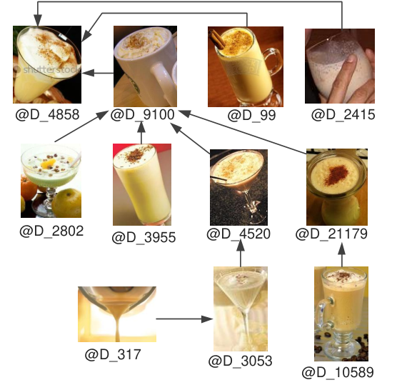
Apart from the accuracy and efficiency, LaPOLeaF discovered the subtle evolution within a given class (see Fig. 2). Thus, as a new GSSL, LaPOLeaF has good interpretability.

The water quality datasets are sampled in Chongqing, China, from March 3rd to November 21st in 2014. The sampling frequency is once per 15 minutes. We choose the PH and DO (dissolved oxygen) index to predict, and compare the performance of LaPOLeaF with least square support vector regression (LSSVR) Suykens et al. (2002) — a classic model that has been widely applied in ecological environment Adnan et al. (2017); Goyal et al. (2014).

Water quality data are time series. We first fold both the PH and DO data as vectors of dimensionality 6 and 13, then regard the first 5 or 12 elements as observed attributes $x$ and the last element as response variable $y$. Thus, dataset Water(PH) is transformed into PH-5Attr and PH-12Attr, and similarly the dataset Water(DO). The first 10,000 records are taken as training set and the succeeding 1000 as test set. The parameter configuration used for LSSVR is $\{\gamma=0.5,\lambda=5,p=3\}$, while that for LaPOLeaF can be found in Table 3.

We will evaluate the performance of prediction via summation of squared error (SSE), which is defined as $SSE=\sum\nolimits_{i}{{{({y_{i}}-{{\widehat{y}}_{i}})}^{2}}}$, where ${y_{i}}$ is the ground truth and ${\widehat{y}}_{i}$ is the predicted value. Table 7 shows the accuracy and efficiency of the two competing methods. The training of LaPOLeaF is faster than LSSVR. However, the prediction of LSSVR is faster than LaPOLeaF, because LSSVR directly computes the estimated value through a formula once the parameters are learned. By contrast, LaPOLeaF needs an $O(N)$ complexity to update the OLeaF with a new observed pattern. For example, when we perform prediction on the PH-12Attr dataset, LSSVR takes 2ms and LaPOLeaF takes 5ms. Although slower, LaPOLeaF could definitely meet the real-time-prediction requirement.

Also, the differences of the true value and the predicted valued are visualized in Fig. 3, from which one can read that LaPOLeaF can approximate the ground truth value on both Water(PH) and Water(DO) datasets. On the dataset Water(DO), LaPOLeaF out performs LSSVR substantially. On Water(PH), LaPOLeaF achieved a slightly lower accuracy than LSSVR, yet the results are comparable. The possible reason for the different performances may be attributed to the spirit of the two methods.

References

- Adnan et al. [2017] Rana Muhammad Adnan, Xiaohui Yuan, Ozgur Kisi, and Rabia Anam. Improving accuracy of river flow forecasting using lssvr with gravitational search algorithm. Advances in Meteorology, 2017(3):1–23, 2017.
- Chen et al. [2018] Dong-Dong Chen, Wei Wang, Wei Gao, and Zhi-Hua Zhou. Tri-net for semi-supervised deep learning. In Proceedings of the 27th International Joint Conference on Artificial Intelligence, pages 2014–2020. AAAI Press, 2018.
- Du et al. [2018] B. Du, X. Tang, Z. Wang, L. Zhang, and D. Tao. Robust graph-based semisupervised learning for noisy labeled data via maximum correntropy criterion. IEEE Transactions on Cybernetics, pages 1–14, 2018.
- Goyal et al. [2014] Manish Kumar Goyal, Birendra Bharti, John Quilty, Jan Adamowski, and Ashish Pandey. Modeling of daily pan evaporation in sub tropical climates using ann, ls-svr, fuzzy logic, and anfis. Expert Systems with Applications, 41(11):5267–5276, 2014.
- Jia et al. [2014] Yangqing Jia, Evan Shelhamer, Jeff Donahue, Sergey Karayev, Jonathan Long, Ross Girshick, Sergio Guadarrama, and Trevor Darrell. Caffe: Convolutional architecture for fast feature embedding. pages 675–678, Nov 2014.
- Li et al. [2019] Feijiang Li, Yuhua Qiana, Jieting Wang, Chuangyin Dang, and Liping Jing. Clustering ensemble based on sample’s stability. Artificial Intelligence, pages 1–23, 2019.
- Liu et al. [2010] Wei Liu, Junfeng He, and Shih-Fu Chang. Large graph construction for scalable semi-supervised learning. In Proceedings of the 27th international conference on machine learning (ICML-10), pages 679–686, 2010.
- Luxburg [2007] Ulrike Von Luxburg. A tutorial on spectral clustering. Statistics and Computing, 17(4):395–416, 2007.
- Ng et al. [2001] A. Y. Ng, M. I. Jordan, and Y. Weiss. On spectral clustering: Analysis and an algorithm. In Proceedings of the 14th International Conference on Neural Information Processing Systems: Natural and Synthetic, 2001.
- Ni et al. [2012] Bingbing Ni, Shuicheng Yan, and Ashraf Kassim. Learning a propagable graph for semisupervised learning: Classification and regression. IEEE Transactions on Knowledge and Data Engineering, 24(1):114–126, 2012.
- Pedrycz and Homenda [2013] Witold Pedrycz and Wladyslaw Homenda. Building the fundamentals of granular computing: A principle of justifiable granularity. Applied Soft Computing, 13(10):4209–4218, 2013.
- Pedrycz et al. [2015] Witold Pedrycz, Giancarlo Succi, Alberto Sillitti, and Joana Iljazi. Data description: A general framework of information granules. Knowledge-Based Systems, 80:98–108, 2015.
- Rodriguez and Laio [2014] A. Rodriguez and A. Laio. Clustering by fast search and find of density peaks. Science, 344(6191):1492–1496, 2014.
- Roweis and Saul [2000] S T Roweis and L K Saul. Nonlinear dimensionality reduction by locally linear embedding. Science, 290(5500):2323–2326, 2000.
- Suykens et al. [2002] J A K Suykens, T V Gestel, J De Brabanter, B De Moor, and J. Vandewalle. Least Squares Support Vector Machines. World Scientific, 2002.
- Wang et al. [2017] Meng Wang, Weijie Fu, Shijie Hao, Hengchang Liu, and Xindong Wu. Learning on big graph: Label inference and regularization with anchor hierarchy. IEEE Transactions on Knowledge and Data Engineering, 29(5):1101–1114, 2017.
- Xu et al. [2016] Ji Xu, Guoyin Wang, and Weihui Deng. DenPEHC: Density peak based efficient hierarchical clustering. Information Sciences, 373:200–218, 2016.
- Xu et al. [2017] Ji Xu, Guoyin Wang, Tianrui Li, Weihui Deng, and Guanglei Gou. Fat node leading tree for data stream clustering with density peaks. Knowledge-Based Systems, 120:99–117, 2017.
- Xu et al. [2018] Ji Xu, Guoyin Wang, Tianrui Li, and Witold. Pedrycz. Local density-based optimal granulation and manifold information granule description. IEEE Transactions on Cybernetics, 48(10):2795–2808, 2018.
- Zhang and Zhou [2018] Teng Zhang and Zhi-Hua Zhou. Semi-supervised optimal margin distribution machines. In IJCAI, pages 3104–3110, 2018.
- Zhou et al. [2004] Dengyong Zhou, Olivier Bousquet, Thomas N Lal, Jason Weston, and Bernhard Schölkopf. Learning with local and global consistency. In Advances in neural information processing systems, pages 321–328, 2004.
- Zhu et al. [2017] X. Zhu, W Pedrycz, and Z. Li. Granular data description: Designing ellipsoidal information granules. IEEE Transactions on Cybernetics, 47(12):4475–4484, 2017.