An exactly solvable BCS-Hubbard Model in arbitrary dimensions

Introduction—Exact solutions of quantum interacting-particle models in dimensions $>1$ are rare and are important resources for understanding the physics of strongly-correlated systems in dimensions $>1$[1, 2, 3, 4, 5, 6, 7, 8, 9, 10, 11, 12, 13]. More recently, a major advance in understanding the mathematics of topological order was put forth by the introduction of the exactly solvable Toric Code[14] and honeycomb[15, 16, 17, 18] models by Kitaev and their generalizations[19, 20, 21, 22, 23, 24, 25, 26, 27]. The exact solvability of the Kitaev honeycomb model is a result of the existence of an infinite number of conserved quantities (for an infinite lattice) in the model. In this paper, we show that Kitaev’s construction can be generalized to a class of $S=1/2$ lattice fermion models that describe p-wave BCS superconductors with equal spin pairing and with on site Hubbard interaction $U$. The generalization is based on the observation that the Kitaev honeycomb lattice model can be expressed in terms of spinless fermion model[17, 18] via a Jordan-Wigner transformation. The “generalized” lattice fermion models carry both “quasi-particle” and “solitonic” excitations as in the Kitaev honeycomb model except that the solitonic excitations are in general non-topological in lattice fermion models.

To illustrate, we consider in this paper a particular BCS-Hubbard model with equal spin pairing [28, 29, 30] on cubic (3D) and square (2D) lattices. The more general constructions are discussed at the end of the paper.

Model—The Hamiltonian for our BCS-Hubbard model is given by $H=H_{0}+H_{int}$, where

where $\langle i,j\rangle$ describes nearest neighbor sites with $i\in A,j\in B$ being lattices sites belonging to different sublattices of the cubic or square lattice. $t_{ij}=t_{ji}$ and $\Delta_{ij}=-\Delta_{ji}$ are hopping matrix and BCS-pairing term between sites $i$ and $j$, respectively. The last term describes on-site Hubbard interaction $U$ where $l\in A,B$, i.e. all lattices sites where $n_{l\sigma}=c^{\dagger}_{l\sigma}c_{l\sigma}$. Notice that the BCS-pairing term describes equal spin pairing. We shall consider a pairing term $\Delta_{ij}$ which is positive when $i\in A,j\in B$, corresponding to a staggering nearest neighbor pairing field on the cubic and square lattices (see Fig.(1) ).

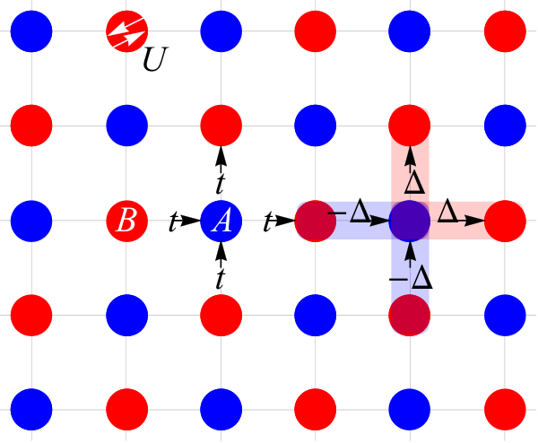
The Hamiltonian (1) is in general not solvable. In the following we shall show that it becomes exactly solvable when $\Delta_{ij}=t_{ij}=t$ where $t$ is a real number.

Construction of exact solution—To see how the model becomes exactly solvable we introduce Majorana fermion representation

for fermions on $i\in A$ and $j\in B$ sublattices, respectively. It is straightforward to show that the Hamiltonian $H$ can be represented in terms of Majorana fermions $\eta$’s and $\beta$’s where

where $t=\tilde{t}(1+\delta)$ and $\Delta=\tilde{t}(1-\delta)$. We notice that in the limit $t=\Delta$ (or $\delta=0$), the kinetic ($H_{0}$) term is expressed in terms of Majorana fermions $\beta$’s only and the $\eta$ terms are absent in $H_{0}$. In this limit,

$\forall l$ and $(2i\eta_{l\uparrow}\eta_{l\downarrow})=D_{l}$ are constants of motion. Using the identities $(\eta_{l\sigma})^{2}=(\beta_{l\sigma})^{2}={1\over 4}$, we obtain $(D_{l})^{2}={1\over 4}$ and $D_{l}=\pm{1\over 2}$.

Substituting $D_{l}$ into Eq. (3), we obtain in the limit $\delta\rightarrow 0$,

where $D_{l}$ are $C$-numbers. The Hamiltonian (4) is quadratic and is exactly diagonalizable. The many-body eigenstates of the Hamiltonian are divided into different solitonic sectors characterized by different sets of eigenvalues $\{D_{l}\}$. The ground state of the system is given by the set of $\{D_{l}\}$ with lowest energy. The construction of the exact solution is parallel to the construction of the exact solution of the spin-$1/2$ Kitaev honeycomb model[15] when the model is expressed in terms of spinless fermions[17, 18]. We show here that the Kitaev construction can be extended to $S=1/2$ lattice fermions with Hubbard-type interaction rather straightforwardly.

Properties of the exact solution (1) - U=0 limit—We first study the solution of Hamiltonian (3) in the limit $U=0$. In this limit $H\rightarrow H_{0}$ describes a p-wave, ESP BCS superconductor with staggered nearest neighbor pairing fields and with chemical potential $\mu=0$, i.e. half-filled bands.

It is convenient to “re-fermionize” the Majorana fermions by introducing the composite fermions

where $\xi_{l}=+(-)1$ for $l\in A(B)-$ sublattices.

The transformation (2) and (5) and be understood by introducing the fermions

which represents fermions with spin pointing in $+(-)\hat{y}-$directions, respectively. The $d$ fermions are related to $c_{\rightleftarrows}$ by

where $d^{(A)}$ and $d^{(B)}$ are fermions on $A(B)$- sublattices, respectively. Eq. (7) represents a Bogoliubov-de Gennes transformation between the $d$ and $c_{\rightleftarrows}$ fermions.

As will be seen below and in next section, the $d$-fermions will form the quasi-particles for our model Hamiltonians. It’s interesting to note from Eq. (7a) that

It is interesting to note from Eq. (8a) that the ($c$)-fermion charges is not directly proportional to the $d$-fermion occupation number, and can be changed only by exciting a pair of $d$ fermions. This is because the $d$-fermions are equal superposition of particle- and hole- states of $c$-fermions. As a result they carry only spin and no charge individually.

In terms of $d$’s, $H_{0}$ becomes

which can be diagonalized straightforwardly by introducing sublattice Fourier transforms

etc., where $\alpha=1,2$ and

with $\Delta_{1}(\mathbf{k})=4it(\sum_{i=1,..dim}\sin k_{i})$ where $dim$ is the dimension of the system and $\Delta_{2}(\mathbf{k})=\delta\Delta_{1}(\mathbf{k})$.

Diagonalizing the Hamiltonian, we obtain

where $E_{\alpha}(\mathbf{k})=|\Delta_{\alpha}(\mathbf{k})|$,

with ground state energy $E_{G}=-\sum_{\mathbf{k}\alpha}E_{\alpha}(\mathbf{k})$.

We notice that $E_{1}(\mathbf{k})\neq E_{2}(\mathbf{k})$, reflecting that the fermion pairing breaks spin-rotation symmetry as can be seen directly from Eq. (9). The spectrum has a Fermi surface denoted by $E_{1(2)}(\mathbf{k})=0$ which describes a rather unusual gapless BCS-superconductor[31].

It is also easy to show that for $\delta\neq 0$,

for $l$ in both sublattices, indicating that the ground state is non-magnetic.

Properties of the exact solution (2) - $U\neq 0$, $\delta=0$—In terms of the composite fermions $d$’s, the Hubbard interaction term can be expressed as,

where $n^{(d)}_{l\rightleftarrows}=d^{\dagger}_{l\rightleftarrows}d_{l\rightleftarrows}$. In the limit $\delta=0$, the Hamiltonian in terms of composite fermions become

(see Eq. (7b) for the relation between 1(2) and $\rightleftarrows$) and $D_{l}=n^{(d)}_{l2}-{1\over 2}=\pm{1\over 2}$ are conserved quantities which can be determined (in the ground state) by minimizing the energy of the system (see discussions after Eq. (3)). We have performed the calculation numerically and find that $D_{l}$ have uniform value $UD_{l}=-{|U|\over 2}$ on the ground state. In particular, the $U$ and $-U$ ground states are related by flipping $D_{l}$ to $-D_{l}$ with the solution for $d_{1}$ fermions remains unchanged.

It may be surprising that although the $d$-fermions carry zero $c$-fermion charge, nevertheless they are affected by the presence of Hubbard-interaction as indicated in Eqs. (13) and (14). To clarify this we construct the on-site states with zero, one and two occupied $d$-fermions, respectively. Using Eq. (7), it is easy to show that

where $|0\rangle$ denotes vacuum for the $c$-fermions, $|0_{d}\rangle$ denotes vacuum for the $d$-fermions, $|s_{d}\rangle$ denotes a state occupied by a single $d$ fermion with spin $s=\rightleftarrows$ and $|\rightleftarrows_{d}\rangle$ denotes a state occupied by two $d$-fermions. Notice that the $c$-fermion number is equal to 1 in all 4 states. However, there exists doubly occupied $c$-fermion state components in states $|0_{d}\rangle$ and $|\rightleftarrows_{d}\rangle$, and they are both affected by the Hubbard interaction $U$.

Fourier transforming, the quasi-particle Hamiltonian (14) in the ground state sector $UD_{l}=-{|U|\over 2}$ can be rewritten as $H=\sum_{\mathbf{k}}\psi^{\dagger}_{\mathbf{k}}h^{(1)}(\mathbf{k})\psi_{\mathbf{k}}$, where $\psi^{\dagger}_{\mathbf{k}\alpha}=(d^{\dagger A}_{\mathbf{k}1},d^{B}_{-\mathbf{k}1})$, and

The quasi-particle energy spectrum for the $d_{1}$ fermions is given by

It is also straightforward to show that

in the ground state for both sublattices $l\in A(B)$ and

is the staggered magnetization carried by the ground state (recall that $d_{1}=d_{\leftarrow(\rightarrow)}$ in sublattices $A(B)$, respectively). We see that the ground state is spin polarized for any $U\neq 0$. The spins are fully polarized in the $U\rightarrow\infty$ limit and the spin polarization approaches zero when $U\rightarrow-\infty$. The singular behavior of magnetization at $U\rightarrow 0$ reflects the singular nature of our Hamiltonian in the $\delta\rightarrow 0$ limit where all $d_{2}$ quasi-particles are localized.

Besides quasi-particle excitations $d_{1}$, we may create solitonic excitations by flipping $D_{l}$’s from ground state. The energy of a single soliton excitation $E_{sol}$ is obtained by calculating the “ground state” energy of Hamiltonian (14) with a singly flipped $D_{l}$. We have performed this calculation numerically in a square lattice for various values of $U/t$ and the results are shown in Fig.(2). We note that the excitation energy is proportional to $U^{2}$ at small $U$ but is proportional to $\tilde{t}^{2}/|U|$ for $|U|\gg\tilde{t}$. Physically, the soliton excitation is created by adding (or subtracting) a localized $d_{2}$ fermion with a dressed cloud of $d_{1}$ fermions. The charge and spin carried by the soliton is calculated using Eq. (8a) and we find that the soliton is chargeless and carries spin $1$ for $U\gtrsim 4\tilde{t}$ and spin $0$ for $U\lesssim-4\tilde{t}$. There exists also a small region around $|U|\lesssim 4\tilde{t}$ where the spin is $1/2$ (see Fig.(2)). Physically, the soliton is a bound state between the $d_{2}$ particle and $d_{1}$ hole when $U/4\tilde{t}$ is large and positive and is a bound state between $d_{2}$ hole and $d_{1}$ hole when $U/4\tilde{t}$ is large and negative. The $d_{1(2)}$ fermions are unbounded when $|U|\lesssim 4\tilde{t}$. Consequently we expect that the soliton is a boson (spin=$0,1$) when $|U|\gtrsim 4\tilde{t}$ and is a spin-$1/2$ fermion when $|U|\lesssim 4\tilde{t}$.

To study the $\delta\rightarrow 0$, $U\rightarrow 0$ region more carefully we show in Fig.(2) the ground state staggered magnetization magnitude as a function of $U/\tilde{t}$ in our square lattice model with $\delta=0.0$ and $0.1$ computed using a mean-field approximation

where we have used Eqs. (6) and (7) in deriving the last equality. The ground state expectation values $\langle(n^{(d)}_{l\rightleftarrows}-{1\over 2})\rangle$ are determined self-consistently from the mean field theory. The mean field result becomes exact in the limit $U=0$ and $U/\delta\rightarrow\infty$ and the $\delta\neq 0$ mean-field calculation provides an extrapolation between the two exact limits. We find that the singular behavior of staggered magnetization $m_{y}$ at $\delta=0$ as given by Eq. (21) is smoothed out for $\delta=0.1$. The excitation energies and spins carried by the solitions for $\delta=0.1$ are also calculated in the mean field theory for different values of $U$ and are shown in Fig.(2) for comparison. We see that both the excitation energies and spins carried by the solition are similar for $\delta=0.0$ and $0.1$.

Summary and discussions—Summarizing, we introduce in this paper an exact solvable BCS-Hubbard model in arbitrary dimensions. The construction of the exact solution is parallel to the exactly solvable Kitaev honeycomb model for $S=1/2$ quantum spins and can be viewed as a generalization of Kitaev’s construction to $S=1/2$ interacting lattice fermions. In fact, any Hamiltonian which when represented in terms of Majorana fermions, has the form

is exactly solvable following our discussion on the construction on exact solution, independent of dimension and lattice structure. The nearest neighbor hopping ($t$) + pairing ($\Delta$) model on square (and cubic) lattices we consider in this paper is just an example of a large class of exactly solvable lattice fermion models that can be written in the form (23). We also notice that the fermionic form Eq.(14) is similar to the Falicov-Kimball model[32, 33].

Physically, the presence of the ESP pairing term $\Delta$ breaks spin rotation symmetry making one of the two quasi-particle bands completely flat in the limit $\delta\rightarrow 0$. The quasi-particles in the flat band are localized making the resulting Hamiltonian exactly solvable. The same happens in the Kitaev honeycomb model. We note that the quasi-particles are non-perturbative objects that are related to the original $c$-fermion states by a local Bogoliubov-de Gennes transformation (7) in our model. As a result the quasi-particle and solitonic excitations both carry non-trivial charge and spin quantum numbers as discussed in the main text.

Lastly we comment that our construction of exactly solvable model suggests a new mean field decoupling channel of Hubbard interaction (22) which can be applied to any interacting fermion model when expressed in terms of Majoranan fermions. The decoupling scheme breaks spin-rotation symmetry and becomes exact when one of the quasi-particle band becomes flat.

Acknowledgment—Z. Chen and X. Li acknowledge Dr. Yao Lu for helpful discussions. This work is supported by Hong Kong RGC through grant HKUST3/CRF/13G.

References

- [1] N. H. March and G. G. Angilella, Exactly Solvable Models in Many-Body Theory (World Scientific, 2016).
- [2] G. D. Mahan, “Exactly solvable models,” in Many-Particle Physics (Springer US, Boston, MA, 2000) pp. 187–294.
- [3] J. Dukelsky, S. Pittel, and G. Sierra, Rev. Mod. Phys. 76, 643 (2004).
- [4] R. Richardson and N. Sherman, Nuclear Physics 52, 221 (1964).
- [5] R. Richardson, Journal of Mathematical Physics 6, 1034 (1965).
- [6] R. Richardson, Journal of Mathematical Physics 9, 1327 (1968).
- [7] G. Sierra, Nuclear Physics B 572, 517 (2000).
- [8] M. Schechter, Y. Imry, Y. Levinson, and J. von Delft, Physical Review B 63, 214518 (2001).
- [9] X.-G. Wen, Phys. Rev. Lett. 90, 016803 (2003).
- [10] S. Vijay and L. Fu, arXiv preprint arXiv:1706.07070 (2017).
- [11] H. Yao, S.-C. Zhang, and S. A. Kivelson, Phys. Rev. Lett. 102, 217202 (2009).
- [12] A. Montorsi and M. Rasetti, Phys. Rev. Lett. 66, 1383 (1991).
- [13] R. K. Ghosh and S. Rao, Physics Letters A 238, 213 (1998).
- [14] A. Kitaev, Annals of Physics 303, 2 (2003).
- [15] A. Kitaev, Annals of Physics 321, 2 (2006).
- [16] G. Baskaran, S. Mandal, and R. Shankar, Phys. Rev. Lett. 98, 247201 (2007).
- [17] H.-D. Chen and Z. Nussinov, Journal of Physics A: Mathematical and Theoretical 41, 075001 (2008).
- [18] X.-Y. Feng, G.-M. Zhang, and T. Xiang, Physical review letters 98, 087204 (2007).
- [19] H. Yao and S. A. Kivelson, Phys. Rev. Lett. 99, 247203 (2007).
- [20] V. Chua, H. Yao, and G. A. Fiete, Phys. Rev. B 83, 180412 (2011).
- [21] I. Mondragon-Shem and T. L. Hughes, Journal of Statistical Mechanics: Theory and Experiment 2014, P10022 (2014).
- [22] G.-W. Chern, Phys. Rev. B 81, 125134 (2010).
- [23] R. Nakai, S. Ryu, and A. Furusaki, Phys. Rev. B 85, 155119 (2012).
- [24] C. Wu, D. Arovas, and H.-H. Hung, Phys. Rev. B 79, 134427 (2009).
- [25] S. Yang, D. L. Zhou, and C. P. Sun, Phys. Rev. B 76, 180404 (2007).
- [26] G. Kells, J. Kailasvuori, J. Slingerland, and J. Vala, New Journal of Physics 13, 095014 (2011).
- [27] M. Hermanns, K. O’Brien, and S. Trebst, Phys. Rev. Lett. 114, 157202 (2015).
- [28] I. Lee, M. Naughton, G. Danner, and P. Chaikin, Physical review letters 78, 3555 (1997).
- [29] G. R. Stewart, Z. Fisk, J. O. Willis, and J. L. Smith, Phys. Rev. Lett. 52, 679 (1984).
- [30] Y. Maeno, H. Hashimoto, K. Yoshida, S. Nishizaki, T. Fujita, J. Bednorz, and F. Lichtenberg, Nature 372, 532 (1994).
- [31] M. Hermanns and S. Trebst, Phys. Rev. B 89, 235102 (2014).
- [32] L. M. Falicov and J. C. Kimball, Phys. Rev. Lett. 22, 997 (1969).
- [33] C. Prosko, S.-P. Lee, and J. Maciejko, arXiv preprint arXiv:1708.08507 (2017).