Impact of Charm H1-ZEUS Combined data and Determination of the Strong Coupling in Two Different Schemes
Abstract
We study the impact of recent measurements of charm cross section H1-ZEUS combined data on simultaneous determination of parton distribution functions (PDFs) and the strong coupling, , in two different schemes. We perform several fits based on Thorne-Roberts (RT) and Thorne-Roberts optimal (RTOPT) schemes at next-to-leading order (NLO). We show that adding charm cross section H1-ZEUS combined data reduces the uncertainty of the gluon distribution and improves the fit quality up to % and % , without and with the charm contribution, from the RT scheme to the RTOPT scheme, respectively. We also emphasise the central role of the strong coupling, , in revealing the impact of charm flavour contribution, when it is considered as an extra free parameter. We show that in going from the RT scheme to the RT OPT scheme, we get % and % improvement in the value of , without and with the charm flavour contribution respectively.
pacs
12.38.AwI Introduction
When the mass of a quark is significantly larger than the quantum chromodynamics (QCD) scale parameter, MeV, we categorize it as a heavy quark [1]. The production of heavy quarks in photoproduction () and deep inelastic scattering (DIS) of was one of the main tasks at HERA. The only heavy quarks kinematically accessible at HERA were beauty and charm quarks, and investigation of the impact of charm quark cross section H1-ZEUS combined data [2] on simultaneous determination of parton distribution functions and the strong coupling, , is the main topic of this analysis. In deep inelastic scattering we can approximate the ratio of photon couplings corresponding to a heavy quark, , by
| (1) |
where are the beauty and charm electric charges, respectively, and , with , represent the kinematically accessible quark flavours.
Now, for the charm quark we have
| (2) |
From Eq. 2 we see that up to 36 percent of the cross sections at HERA originate from processes with charm quarks in the final state. This is our main motivation to investigate the impact of only charm quarks on simultaneous determination of parton distribution functions or their uncertainties and the strong coupling, .
The ratio implies that charm quarks are an integral part of the quark-antiquark sea within the proton. On the other hand, the proton has no net charm flavour number, which in turn implies that the charm quarks within the proton can only arise in pairs of . Since the charm-quark mass is about GeV , at the low-energy limit the pairs are considerably heavier than that to have a contribution within the proton.
Although consideration of so-called intrinsic charm (IC) [3] may alter this simple view of the heavy flavour content of the proton, at present there is no evidence for the existence of such a contribution from HERA data. Therefore, in this analysis the charm quarks within the proton are as usual considered as virtual quarks, which in turn arise as fluctuations of probing the gluon content of the proton.
The charm PDFs play an important role in hadronic collisions and cause photons to emerge from hard parton-parton interactions in association with one or more charm quark jets. Clearly, to study and analyse these processes, we need the charm PDFs, which in turn have sizeable uncertainties. A series of experimental measurements involving charm (or beauty) and photon final states have recently been published by the CDF and D0 Collaborations [4, 5, 6, 7, 8, 9].
As we noted, the charm quark mass is about GeV , whereas the QCD scale is about GeV , so it is reasonable to treat the charm quark mass as a hard scale in perturbative quantum chromodynamics (pQCD) and investigate the charm mass effect in pQCD. Accordingly, in this study we use the full HERA run I and II combined data [10] as a new measurements of inclusive deep inelastic scattering cross sections for our base data set and then we investigate, simultaneously, the impact of charm quark cross section H1-ZEUS combined data [2] on the central value of the PDFs and determination of the strong coupling, .
Although the charm quark mass is large compared to the QCD scale, it is small with respect to other pQCD scales, such as the transverse momentum of a quark or a jet, , and the virtuality of the photon, . This smallness leads to the logarithmic correction terms, and , corresponding to and , respectively. At present, the order of magnitude and treatment of these correction terms are open questions.
The outline of this paper is as follows. In Section 2, we describe the theoretical framework of our study and discuss the reduced cross sections. We introduce the data set which we use in this QCD-analysis and discuss our methodology in Section 3. In Section 4, the impact of charm quark cross section H1-ZEUS combined data on QCD fit quality is discussed. We explain the impact of charm production data on PDFs and in Section 5. We present our results in Section 6 and conclude with a summary in Section 7.
II Cross sections and parton distributions
In perturbative quantum chromodynamics, the deep inelastic scattering of , at the centre-of-mass energies up to GeV at HERA, plays a central role in probing the structure of the proton, as a sea of strongly interacting quarks and gluons. For neutral current (NC) interactions, the reduced cross sections can be expressed in terms of the generalized structure functions as:
| (3) | |||||
where and is the fine-structure constant which is defined at zero momentum transfer. The generalized structure functions , and can be expressed as linear combinations of the proton structure functions and as follows:
| (4) |
where and are the vector and axial-vector weak couplings of the electron to the boson, and is defined as
| (5) |
This analysis is based on xFitter, an open source QCD framework [11] which is an update of the former HERAFitter package [12]. The values of the -boson mass and the electroweak mixing angle are GeV and , respectively, and electroweak effects have been treated only at leading order (LO).
In the range of low values of , , the boson exchange contribution may be ignored and then the reduced NC DIS cross sections can be expressed by
| (6) |
Similarly, the reduced charged current (CC) deep inelastic scattering cross sections may be expressed as follows:
| (7) | |||||
where , and are another set of structure functions and is the Fermi constant, which is related to the weak coupling constant and electromagnetic coupling constant by:
| (8) |
The values of the Fermi constant and -boson mass in the xFitter QCD framework [11] are: GeV-2 and GeV.
In the quark parton model (QPM), the sums and differences of quark and anti-quark distributions, depending on the charge of the lepton beam, can be represented by , structure functions, respectively, and :
| (9) |
According to Eq. 9 we have:
| (10) |
Now it is possible to determine both the valence-quark distributions, and , and the combined sea-quark distributions, and , by combination of NC and CC measurements.
In analogy to the inclusive NC deep inelastic cross section, the reduced cross sections for charm-quark production, , can be expressed by
| (11) | |||||
where , is the electromagnetic coupling constant, and , and are charm-quark contributions to the inclusive structure functions , and , respectively.
In the kinematic region at HERA, the structure function makes a dominant contribution. The structure function contributes only from exchange and , which implies that for the region, this contribution may be ignored. Finally, the contribution of longitudinal charm-quark structure function, , is suppressed only for the region which can be a few percent in the kinematic region accessible at HERA and therefore cannot be ignored.
Therefore, neglecting the structure function contribution, the reduced charm-quark cross section, , for both positron and electron beams, can be expressed by
| (12) | |||||
Accordingly, at high , the reduced charm-quark cross section, , and the structure function only differ by a small contribution [13].
In the QPM, the structure functions depend only on the variable and then they can be directly related to the PDFs. In QCD, however, and especially when heavy flavour production is included, the structure functions depend on both and variables, [14, 15, 16, 17, 18, 19, 20, 21, 22, 23, 24, 25, 26, 27, 28, 29, 30, 31, 32, 33, 34, 35, 36, 37, 38, 39]. In Section III, based on our methodology, we extract the PDFs as functions of and variables, using full HERA run I and II combined data, with and without the charm cross section H1-ZEUS combined measurements data set included.
III Data Set and Methodology
In this paper, we use two different data sets: the full HERA run I and II combined NC and CC DIS scattering cross sections [10], and the charm production reduced cross section measurements data [2]. In our analysis, we choose the full HERA run I and II combined data as our base data set, and then we investigate the impact of charm production reduced cross section data on simultaneous determination of PDFs and the strong coupling, in the Thorne-Roberts (RT) and Thorne-Roberts optimal (RTOPT) schemes. The kinematic ranges for these two data sets have been reported in Ref. [40].
We use xFitter [11], version 1.2.2, as our QCD fit framework. Using the QCDNUM package [41], version 17-01/12, we evolved the parton distribution functions and . In the evolution of PDFs and , we set our theory type based on the DGLAP collinear evolution equations [42] and make several fits at leading order and next-to-leading order in the RT and RTOPT schemes.
The RT scheme is a General Mass-Variable Flavour Number Scheme (GM-VFNS). Really, the RT scheme was designed to provide a smooth transition from the massive FFN scheme at low scales to the massless ZM-VFNS scheme at high scales . However, the connection is not unique. A GM-VFNS can be defined by demanding equivalence of the (FFNS) and flavour (ZM-VFNS) descriptions above the transition point for the new parton distributions. Of course they are by definition identical below this point, at all orders. The RT scheme has two different variants: RT standard and RT optimal, with a smoother transition across the heavy flavour threshold region. A review of the two different schemes has been given in Ref. [40].
To investigate the impact of charm production reduced cross section data, we need to use the heavy flavour scheme in our analysis. Different theoretical groups use various heavy flavour schemes. For example, some theory groups such as CT10 [43], ABKM09 [44], and NNPDF2.1 [45, 46] used S-ACOT [47], FFNS [48] and FONLL [49], respectively and some other groups such as MSTW08 [50] and HERAPDF1.5/2.0 [20] used the RT (also referred to as TR) standard and optimal heavy flavour schemes [51, 52] to calculate the reduced charm cross sections in DIS. On the other hand, to include heavy flavour contributions, the perturbative QCD scales and play a central rule. Some groups such as CT10 [43] and ABKM09 [44] choose and respectively, where denotes the pole mass of the charm quark, whereas the NNPDF2.1 [45, 46], HERAPDF1.5 [20] and MSTW08 [50] groups use in their heavy quark QCD approach.
To include the heavy-flavor contributions, we use both RT and RTOPT schemes, and choose as the perturbative quantum chromodynamics scale for the pole mass of the charm quark GeV.
The last step in our QCD analysis is the minimization procedure. In this regard, we use the standard MINUIT minimization package [53], as a powerful program for minimization, correlations and parameter errors.
In order to minimize the influence of higher twist contributions we use kinematic cuts. In the various DIS analyses, different kinds of kinematic cuts should be applied. In this analysis we imposed a kinematic cut =3.5 GeV2 to omit all data with less than this value. The cuts on the kinematic coverage of the DIS data have been made for values of between GeV2 and GeV2 and values of between and . The cuts on not only significantly increase the number of data points available to constrain PDFs, but also allow access to a greater range of kinematics, which in turn lead to reduced PDF uncertainties, especially at higher values of .
In this analysis, based on the HERAPDF approach [10], we generically parameterized the PDFs of the proton, , at the initial scale of the QCD evolution GeV2 as
| (13) |
where in the infinite momentum frame, is the fraction of the proton’s momentum taken by the struck parton.
To determine the normalization constants for the valence and gluon distributions, we use the QCD number and momentum sum rules. Using this functional form, Eq. 13 leads to the following independent combinations of parton distribution functions:
| (14) | |||||
| (15) | |||||
| (16) | |||||
| (17) | |||||
| (18) |
where is the gluon distribution, and are the valence-quark distributions, and and are the -type and -type anti-quark distributions, which are identical to the sea-quark distributions. A review of HERAPDF functional form, including some more details, can be found in Ref. [40].
IV Impact of Charm Production Data on the QCD fit quality
We now investigate the impact of the charm cross section H1-ZEUS combined measurements on simultaneous determination of PDFs and . We also explain how adding these data improve the uncertainty of PDFs, reducing the error bars of some parton distributions, especially gluon distributions and some of their ratios, when the HERA run I and II combined inclusive DIS scattering cross sections data are chosen as a “BASE”. To investigate the fit quality, we use the definition as reported in Ref. [40].
For HERA run I and II combined inclusive DIS scattering cross sections and the charm cross section H1-ZEUS combined measurements, the number of data points are 1307 and 42, respectively. Accordingly, the total number of data points for BASE and BASE plus charm, which we refer to sometimes as “TOTAL”, are 1307 and 1349, respectively. In various configurations, the GeV2 range was covered by the HERA run I and II combined data [10]. The MINUIT parameters are sensitive to the value, so to get a convergent fit result we set GeV2, as suggested in Ref [10]. Clearly, this cut on omits all data with less than GeV2 and therefore, reduces the total number of data points from 1307 and 1349 to 1145 and 1192 for the BASE and TOTAL data sets, respectively. Now, based on Table 1, we can present our QCD fit quality as follows:
for the RT scheme:
| / dof = for BASE ,
|
(19) | ||
| / dof = for TOTAL ,
|
(20) |
and for the RTOPT scheme:
| / dof = for BASE ,
|
(21) | ||
| / dof = for TOTAL ,
|
(22) |
where dof refers to the per degrees of freedom and is defined as the number of data points minus the number of free parameters. As we can see from Eqs. (19-22), we obtain four different values of /dof, corresponding to four different fits, which in turn imply four different fit-qualities in some PDFs. Now, according to the relative change of , which is defined by and the numerical results of Eqs. (19-22), we see that in going from the RT scheme to the RT OPT scheme, we get % and % improvement in the fit quality, without and with the charm flavour contribution, respectively. Clearly these differences in fit quality imply a significant reduction of some PDF uncertainties, especially for gluon distributions, as we will explain in the next section.
| Order | NLO | |||
|---|---|---|---|---|
| Experiment | RT BASE | RT TOTAL | RTOPT BASE | RTOPT TOTAL |
| HERA I+II CC [10] | 44 / 39 | 45 / 39 | 44 / 39 | 44 / 39 |
| HERA I+II CC [10] | 49 / 42 | 49 / 42 | 50 / 42 | 49 / 42 |
| HERA I+II NC [10] | 221 / 159 | 221 / 159 | 221 / 159 | 221 / 159 |
| HERA I+II NC 460 [10] | 208 / 204 | 209 / 204 | 210 / 204 | 210 / 204 |
| HERA I+II NC 575 [10] | 213 / 254 | 213 / 254 | 212 / 254 | 212 / 254 |
| HERA I+II NC 820 [10] | 66 / 70 | 66 / 70 | 65 / 70 | 66 / 70 |
| HERA I+II NC 920 [10] | 422 / 377 | 424 / 377 | 418 / 377 | 419 / 377 |
| Charm H1-ZEUS [2] | - | 40 / 47 | - | 38 / 47 |
| Correlated | 111 | 122 | 111 | 119 |
| Total / dof | ||||
V Impact of Charm Production Data on PDFs and
Now, we present the impact of charm cross section H1-ZEUS combined measurements data on simultaneous determination of PDFs and in the RT and RTOPT schemes and for two separate scenarios. In the first scenario we fix to 0.117 and develop our QCD fit analysis based on only 14 unknown free parameters, according to Eqs. (14-18). Although in this scenario the value of / dof is reduced, according to Eqs. (19-22), from 1.180 to 1.169, we find nothing to show the impact of charm cross section H1-ZEUS combined measurements data on the PDFs. In the second scenario we consider the strong coupling as an extra free parameter and refit our analysis, but this time with 15 unknown free parameters. Based on the second scenario, not only do we obtain % and % improvement in the fit quality, without and with the charm flavour contribution, respectively, the same as the first scenario, but we also clearly find the impact of charm on the PDFs, especially on the gluon distribution. Some more details about the central role of the strong coupling in pQCD have been reported in Ref. [40].
In Tables 2 and 3, we present next-to-leading order numerical values of parameters and their uncertainties for the , , sea and gluon PDFs at the input scale of GeV2 for the two different scenarios.
| First Scenario: The Strong Coupling, , is Fixed | ||||
|---|---|---|---|---|
| Parameter | RT BASE | RT TOTAL | RTOPT BASE | RTOPT TOTAL |
| Second Scenario: The Strong Coupling, , is Free | ||||
|---|---|---|---|---|
| Parameter | RT BASE | RT TOTAL | RTOPT BASE | RTOPT TOTAL |
According to the numerical results in Table 3, when we add the charm cross section H1-ZEUS combined measurements data to the HERA run I and II combined data, the numerical value of changes from to and from to , for the RT and RTOPT schemes, without and with charm flavour data included, respectively. If we compare our results for for RT TOTAL and RTOPT TOTAL with the world average value, , which was recently reported by the PDG [33], we find a good agreement with the world average value. Of course, it should be noted, since the PDG value of is extracted by global fits to a variety of experimental data, it has a much smaller uncertainty. In other words, although our QCD analysis has been performed based on only two data sets, our numerical results for the strong coupling are in good agreement with the world average value. Also, these values of strong coupling show the impact of the RT and RTOPT schemes on the determination of , when considered as an extra free parameter.
VI Results
According to Table 4, in going from the RT scheme to the RTOPT scheme, we get % and % improvement in the fit quality, without and with the charm flavour contributions included, respectively. Also, according to Table 5, in going from the RT scheme to the RTOPT scheme, we get % and % improvement in the value, without and with the charm flavour contributions respectively.
| First Scenario: The Strong Coupling, is Fixed | ||
|---|---|---|
| Scheme | ||
| RT BASE | ||
| RT TOTAL | ||
| RTOPT BASE | ||
| RTOPT TOTAL | ||
| Second Scenario: The Strong Coupling, is Free | ||
|---|---|---|
| Scheme | ||
| RT BASE | ||
| RT TOTAL | ||
| RTOPT BASE | ||
| RTOPT TOTAL | ||
In Fig. 1, we illustrate the consistency of HERA measurements of the reduced deep inelastic scattering cross sections data [10] and charm production reduced cross section measurements data [2] with the theory predictions as a function of and for different values of . According to our QCD analysis, we have good agreement between the theoretical and experimental data. The uncertainties on the cross sections in Fig. 1 are obtained using Hessian error propagation. The corresponding values for each of the data sets in Fig. 1 are listed in Table 1.


The impact of charm cross section H1-ZEUS combined measurements data on HERA I and II combined data for gluon distribution functions are shown in Figs. 2 and 3, at the starting value of = 1.9 GeV2 and = 3, 4 and 5 GeV2, in the RT and RTOPT schemes and for two separate scenarios. Clearly, in the first scenario, where the strong coupling is fixed, we find no impact from adding charm H1-ZEUS combined data to the HERA I and II combined data. In the second scenario, however, where we consider the strong coupling as an extra free parameter, we clearly find the impact of adding charm H1-ZEUS combined data to the HERA I and II combined data.


The partial gluon distribution functions are shown in Figs. 4 and 5, at = 1.9, 3, 5 and 10 GeV2 in the RT and RTOPT schemes and for two separate scenarios. The impact of adding charm H1-ZEUS combined data to the HERA I and II combined data can be seen only in the second scenario, where the strong coupling, , is considered as an extra free parameter.


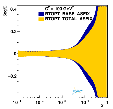
The total sea quark -PDFs are defined by . In Figs. 6 and 7 we plot the partial ratio of gluon distributions over the -PDF to show the impact of adding charm cross section H1-ZEUS combined data to HERA I and II combined data, at = 4, 5, 100 and 10000 GeV2 in the RT and RTOPT schemes and for the two different scenarios. Clearly, these impacts can be seen only in the second scenario.




VII Summary
Up to 36 percent of the cross sections at HERA originate from processes with charm quarks in the final state. In this QCD analysis we investigated the simultaneous impact of charm quark cross section H1-ZEUS combined data on the PDFs and on the determination of the strong coupling.
We chose the full HERA run I and II DIS charged and neutral current data as a base data set and developed our QCD analysis at next-to-leading order in both RT and RTOPT schemes and for two separate scenarios using the HERAPDF parametrization form.
The sensitivity of PDF uncertainties to reduced charm quark cross section H1-ZEUS combined data at next-to-leading order, especially when in our second scenario we take the strong coupling, , as an extra free parameter, is reported in this QCD analysis.
This analysis shows a dramatic reduction of some PDF uncertainties and good agreement of the strong coupling constant, , with the world average value, when the reduced charm quark cross section H1-ZEUS combined data are included.
As we mentioned, the strong coupling, , plays a central role in the pQCD factorization theorem and the result of this QCD-analysis emphasis on its dramatic correlation with the PDFs reveals the impact of the charm flavour contribution.
According our QCD analysis, in going from the RT scheme to the RTOPT scheme, we get % and % improvement in the fit quality, without and with the charm flavour contribution, respectively. Also, we show that in going from the RT scheme to the RTOPT scheme, we get % and % improvement in the strong coupling value, without and with the charm flavour contribution, respectively.
A standard LHAPDF library file of this QCD analysis at next-to-leading order is available and can be obtained from the author via e-mail.
References
- [1] O. Behnke, A. Geiser and M. Lisovyi, Prog. Part. Nucl. Phys. 84, 1 (2015) [arXiv:1506.07519 [hep-ex]].
- [2] H. Abramowicz et al. [H1 and ZEUS Collaborations], Eur. Phys. J. C 73, no. 2, 2311 (2013) [arXiv:1211.1182 [hep-ex]].
- [3] S. J. Brodsky, P. Hoyer, C. Peterson and N. Sakai, Phys. Lett. 93B, 451 (1980).
- [4] V. M. Abazov et al. [D0 Collaboration], Phys. Lett. B 714, 32 (2012) [arXiv:1203.5865 [hep-ex]].
- [5] V. M. Abazov et al. [D0 Collaboration], Phys. Rev. Lett. 102, 192002 (2009) [arXiv:0901.0739 [hep-ex]].
- [6] V. M. Abazov et al. [D0 Collaboration], Phys. Lett. B 719, 354 (2013) [arXiv:1210.5033 [hep-ex]].
- [7] V. M. Abazov et al. [D0 Collaboration], Phys. Lett. B 737, 357 (2014) [arXiv:1405.3964 [hep-ex]].
- [8] T. Aaltonen et al. [CDF Collaboration], Phys. Rev. D 81, 052006 (2010) [arXiv:0912.3453 [hep-ex]].
- [9] T. Aaltonen et al. [CDF Collaboration], Phys. Rev. Lett. 111, no. 4, 042003 (2013) [arXiv:1303.6136 [hep-ex]].
- [10] H. Abramowicz et al. [H1 and ZEUS Collaborations], Eur. Phys. J. C 75, no. 12, 580 (2015) [arXiv:1506.06042 [hep-ex]].
- [11] xFitter, An open source QCD fit framework. http://xFitter.org [xFitter.org] [arXiv:1410.4412 [hep-ph]].
- [12] A. Sapronov [HERAFitter Team Collaboration], J. Phys. Conf. Ser. 608, no. 1, 012051 (2015).
- [13] K. Daum, S. Riemersma, B. W. Harris, E. Laenen and J. Smith, In *Hamburg 1995/96, Future physics at HERA* 89-101 [hep-ph/9609478].
- [14] T. Sjostrand, L. Lonnblad and S. Mrenna, hep-ph/0108264.
- [15] A. Aktas et al. [H1 Collaboration], Eur. Phys. J. C 48, 715 (2006) [hep-ex/0606004].
- [16] A. De Roeck and R. S. Thorne, Prog. Part. Nucl. Phys. 66, 727 (2011) [arXiv:1103.0555 [hep-ph]].
- [17] R. D. Ball, L. Del Debbio, S. Forte, A. Guffanti, J. I. Latorre, J. Rojo and M. Ubiali, Nucl. Phys. B 838, 136 (2010) [arXiv:1002.4407 [hep-ph]].
- [18] F. D. Aaron et al. [H1 Collaboration], Eur. Phys. J. C 71, 1769 (2011) Erratum: [Eur. Phys. J. C 72, 2252 (2012)] [arXiv:1106.1028 [hep-ex]].
- [19] W. K. Tung, H. L. Lai, A. Belyaev, J. Pumplin, D. Stump and C.-P. Yuan, JHEP 0702, 053 (2007) [hep-ph/0611254].
- [20] F. D. Aaron et al. [H1 and ZEUS Collaborations], JHEP 1001, 109 (2010) [arXiv:0911.0884 [hep-ex]].
- [21] J. Engelen and P. Kooijman, Prog. Part. Nucl. Phys. 41, 1 (1998).
- [22] A. Cooper-Sarkar, J. Phys. G 39, 093001 (2012) [arXiv:1206.0894 [hep-ph]].
- [23] S. Frixione, M. L. Mangano, P. Nason and G. Ridolfi, Phys. Lett. B 319, 339 (1993) [hep-ph/9310350].
- [24] G. Marchesini, B. R. Webber, G. Abbiendi, I. G. Knowles, M. H. Seymour and L. Stanco, Comput. Phys. Commun. 67, 465 (1992).
- [25] H. Jung, Comput. Phys. Commun. 86, 147 (1995).
- [26] T. Sjostrand, Comput. Phys. Commun. 39, 347 (1986).
- [27] T. Sjostrand and M. Bengtsson, Comput. Phys. Commun. 43, 367 (1987).
- [28] L. Lonnblad, Comput. Phys. Commun. 71, 15 (1992).
- [29] E. A. Kuraev, L. N. Lipatov and V. S. Fadin, Sov. Phys. JETP 44, 443 (1976) [Zh. Eksp. Teor. Fiz. 71, 840 (1976)].
- [30] M. Ciafaloni, Nucl. Phys. B 296, 49 (1988).
- [31] H. Jung and G. P. Salam, Eur. Phys. J. C 19, 351 (2001) [hep-ph/0012143].
- [32] M. Beneke, Phys. Lett. B 344, 341 (1995) [hep-ph/9408380].
- [33] K. A. Olive et al. [Particle Data Group], Chin. Phys. C 38, 090001 (2014).
- [34] B. Schmidt and M. Steinhauser, Comput. Phys. Commun. 183, 1845 (2012) [arXiv:1201.6149 [hep-ph]].
- [35] S. Alekhin and S. Moch, Phys. Lett. B 699, 345 (2011) [arXiv:1011.5790 [hep-ph]].
- [36] J. Gao, M. Guzzi and P. M. Nadolsky, Eur. Phys. J. C 73, no. 8, 2541 (2013) [arXiv:1304.3494 [hep-ph]].
- [37] A. D. Martin, R. G. Roberts, W. J. Stirling and R. S. Thorne, Eur. Phys. J. C 4, 463 (1998) [hep-ph/9803445].
- [38] J. Pumplin, D. R. Stump, J. Huston, H. L. Lai, P. M. Nadolsky and W. K. Tung, JHEP 0207, 012 (2002) [hep-ph/0201195].
- [39] S. Chekanov et al. [ZEUS Collaboration], Phys. Rev. D 67, 012007 (2003) [hep-ex/0208023].
- [40] A. Vafaee and A. N. Khorramian, Nucl. Phys. B 921, 472 (2017).
- [41] M. Botje, Comput. Phys. Commun. 182, 490 (2011) [arXiv:1005.1481 [hep-ph]].
- [42]
V. N. Gribov and L. N. Lipatov,
Sov. J. Nucl. Phys. 15, 438 (1972)
[Yad. Fiz. 15, 781 (1972)];
L. N. Lipatov, Sov. J. Nucl. Phys. 20, 94 (1975) [Yad. Fiz. 20, 181 (1974)];
Y. L. Dokshitzer, Sov. Phys. JETP 46, 641 (1977) [Zh. Eksp. Teor. Fiz. 73, 1216 (1977)];
G. Altarelli and G. Parisi, Nucl. Phys. B 126, 298 (1977). - [43] H. L. Lai, M. Guzzi, J. Huston, Z. Li, P. M. Nadolsky, J. Pumplin and C.-P. Yuan, Phys. Rev. D 82, 074024 (2010) [arXiv:1007.2241 [hep-ph]].
- [44] S. Alekhin, J. Blumlein, S. Klein and S. Moch, arXiv:0908.3128 [hep-ph].
- [45] R. D. Ball et al. [NNPDF Collaboration], Nucl. Phys. B 809, 1 (2009) Erratum: [Nucl. Phys. B 816, 293 (2009)] [arXiv:0808.1231 [hep-ph]].
- [46] A. Mironov and A. Morozov, JHEP 1004, 040 (2010) [arXiv:0910.5670 [hep-th]].
- [47] J. C. Collins, Phys. Rev. D 58, 094002 (1998) [hep-ph/9806259].
- [48] A. D. Martin, W. J. Stirling and R. S. Thorne, Phys. Lett. B 636, 259 (2006) [hep-ph/0603143].
- [49] S. Forte, E. Laenen, P. Nason and J. Rojo, Nucl. Phys. B 834, 116 (2010) [arXiv:1001.2312 [hep-ph]].
- [50] A. D. Martin, W. J. Stirling, R. S. Thorne and G. Watt, Eur. Phys. J. C 63, 189 (2009) [arXiv:0901.0002 [hep-ph]].
- [51] R. S. Thorne, Phys. Rev. D 73, 054019 (2006) [hep-ph/0601245].
- [52] R. S. Thorne, Phys. Rev. D 86, 074017 (2012) [arXiv:1201.6180 [hep-ph]].
- [53] F. James and M. Roos, Comput. Phys. Commun. 10, 343 (1975).