On Fractionally-Supervised Classification: Weight Selection and Extension to the Multivariate -Distribution
Abstract
Recent work on fractionally-supervised classification (FSC), an approach that allows classification to be carried out with a fractional amount of weight given to the unlabelled points, is further developed in two respects. The primary development addresses a question of fundamental importance over how to choose the amount of weight given to the unlabelled points. The resolution of this matter is essential because it makes FSC more readily applicable to real problems. Interestingly, the resolution of the weight selection problem opens up the possibility of a different approach to model selection in model-based clustering and classification. A secondary development demonstrates that the FSC approach can be effective beyond Gaussian mixture models. To this end, an FSC approach is illustrated using mixtures of multivariate -distributions.
Keywords: Fractionally-supervised classification; weight selection; multivariate -distribution.
1 Introduction
In a typical classification application, some of the observations are unlabelled and the objective is to predict the labels of the unlabelled points, for details see McNicholas (2016a). In such situations, classification is generally semi-supervised or supervised (also called discriminant analysis). These two species of classification differ in whether any weight is given to the unlabelled points in the prediction of their labels. In semi-supervised classification, the labelled and unlabelled points are given equal weight; however, in supervised classification, the unlabelled points are given zero weight. Furthermore, it is possible to either give all the weight to the unlabelled points or treat all the points as unlabelled. This third, and well known, species of classification is called unsupervised classification or cluster analysis. These three species of classification are well established; yet, in any given scenario, it might be the case that labelled or unlabelled observations are more important when building a classifier.
Vrbik and McNicholas (2015) introduce a general approach, called fractionally-supervised classification (FSC), where classification can be carried out with a fractional amount of weight — anything between none and all — being given to the unlabelled points. This approach allows for an intermediate solution between the three different species of classification. Moreover, although it was conceived in the model-based paradigm with the use of Gaussian mixture models and weighted likelihood, discussed in detail in Section 2, it is more generally applicable and will be illustrated herein for -mixtures.
Vrbik and McNicholas (2015) show that FSC oftentimes improves classification performance when compared to the three different species of classification; however, the problem over how to choose the appropriate amount of weight to give the unlabelled points remains unanswered. Vrbik and McNicholas (2015) discussed a few different options to choose the appropriate weight but all of these procedures were deemed undesirable. Vrbik and McNicholas (2015) ultimately decided to use the adjusted Rand index (Hubert and Arabie, 1985, ARI;) to choose the weight; however, while this approach was sufficient to illustrate that FSC can be very effective, it is not viable in practice because it assumes knowledge of the labels that are treated as unknown in the analysis. The main contribution of the present work is to determine a weight selection criterion that can be used in real problems, where there are genuinely unlabelled points. The secondary contribution of this paper is the demonstration of FSC for non-Gaussian mixture models, in particular the multivariate -distribution.
The remainder of this paper is laid out as follows. In Section 2, a detailed discussion of mixture models, FSC and weighted likelihood, as well as a brief discussion of the multivariate -distribution is presented. Then, FSC with the multivariate -distribution is laid out (Section 3) and a detailed discussion on weight selection criteria is presented (Section 4). In Section 5, simulations and demonstrations using real data are presented and we conclude with a discussion and suggestions for future work (Section 6).
2 Background
2.1 Finite Mixture Models and Model-Based Clustering
McNicholas (2016a) traces the relationship between mixture models and clustering back as far as Tiedeman (1955). The first use of finite mixture models for model-based clustering is generally regarded to be by Wolfe (1965) and, in the intervening years, model-based clustering has become a popular approach for clustering (McNicholas, 2016b, a recent review is given by). A finite mixture model assumes that an observation comes from a population with subgroups. The density function of is given by
| (1) |
where , with , are called the mixing proportions, are the component densities, and .
Because of its mathematical tractability, the Gaussian mixture model has been looked at extensively in the literature. In addition to Wolfe (1965), other examples of earlier work in the area of model-based clustering using Gaussian mixtures include Baum et al. (1970), Scott and Symons (1971) and Orchard and Woodbury (1972). For more details on the history of model based clustering, see McNicholas (2016b). More recently, there has also been a fair amount of work using non-Gaussian mixtures such as the -distribution (Peel and McLachlan, 2000; Andrews and McNicholas, 2011a; Andrews and McNicholas, 2011b; Andrews and McNicholas, 2012; Steane et al., 2012; Lin et al., 2014, e.g.,) and skewed distributions (Lin, 2010; Vrbik and McNicholas, 2012; Vrbik and McNicholas, 2014; Lee and McLachlan, 2013; Lee and McLachlan, 2014; Franczak et al., 2014; Franczak et al., 2015; Dang et al., 2015; Lin et al., 2016; Murray et al., 2014a; Murray et al., 2014b; Murray et al., 2017a; Murray et al., 2017b). Related to this work, an interesting vein of work has been carried out on cluster-weighted models (Ingrassia et al., 2012; Subedi et al., 2013; Ingrassia et al., 2015; Subedi et al., 2015; Punzo and McNicholas, 2017, CWMs; e.g.,).
2.2 Three Species of Classification
Let the matrix be a data matrix, where the are -dimensional vectors and is the number of data points. We can then split into two sub-matrices and , where are data points with known labels, and are observations with unknown labels. Then write . Also, define , to be a matrix of indicator vectors. Specifically, we define , were are -dimensional vectors with elements 0 or 1. For convenience, we will denote element of by where
We can likewise define in the same manner. Furthermore, for are analogous to for the unlabelled observations. Define to be our set of observed data, and to be our complete-data. We can furthermore denote the observed data corresponding to labelled observations by , and the data corresponding to unlabelled observations by .
Using the above notation, we can now describe the three species of classification. The first species is discriminant analysis, which makes use of only labelled data to build a classifier. The likelihood function in the case of a discriminant analysis can be written as
| (2) |
The second species is cluster analysis, and can take on one of two forms. The first form is the one that we will primarily consider, and makes use of only unlabelled data points and ignores the labelled points. In this case, the likelihood function is given by
| (3) |
The second form of the cluster analysis utilizes both labelled and unlabelled points, but treats the labelled points as unlabelled.
The third species is semi-supervised classification. This makes use of all of the observed data and treats labelled and unlabelled points equally when building a classifier. The likelihood function for semi-supervised classification is given by the product of and to give
| (4) |
2.3 Fractionally-Supervised Classification
Introduced by Vrbik and McNicholas (2015), FSC allows for a solution intermediate to the three species of classification. This is achieved by introducing the weight to labelled observations, and to unlabelled observations, where . Using these weights, the most natural form of the weighted observed likelihood can be written as
| (5) |
where is the th element of . Although does not necessarily have to equal , we will make the assumption that . We can then write the complete-data log-likelihood function as
| (6) |
The expectation-maximization (EM) algorithm (Dempster et al., 1977) can then be used to maximize (6). The EM algorithm is an iterative algorithm that, on each iteration, consists of a conditional expectation (E-) step and the subsequent maximization of the expectation (M-step). We first initialize the parameters, and we denote this by . Iteration of the EM algorithm proceeds as follows.
| (7a) | ||||
| (7b) | ||||
| (7c) | ||||
| and return to (7a). | ||||
As was shown in Vrbik and McNicholas (2015), in the case of a Gaussian mixture model, steps (7a) and (7b) simplify to the following.
| E-Step: Update | ||||
| M-Step: Update the estimates of , and by calculating | ||||
This simplified form of the EM algorithm will prove useful when we discuss the EM algorithm in the case of a FSC with mixture of multivariate -distributions (Section 3).
We note that the three different species of classification fall out naturally as special cases of FSC. If , then all of the weight is given to the labelled observations, and the unlabelled observations are ignored. In this case, we are performing discriminant analysis. If , then the labelled and unlabelled observations are given equal weight, and we are then performing semi-supervised classification. Finally, if , then no weight is given to the labelled observations, and thus we are performing a cluster analysis (on the unlabelled observations). As mentioned in Section 1, the main unresolved issue with FSC is the selection of the weight .
2.4 The Multivariate -Distribution
The -dimensional -distribution with degrees of freedom, location parameter and scale matrix , arises as a special case of a normal scale mixture (Peel and McLachlan, 2000). Specifically, we can write the normal scale mixture as
| (9) |
where denotes the multivariate Gaussian density with mean and covariance matrix , and is small. We can then rewrite (9) as
where
| (10) |
and is the gamma function. Note that (10) is the probability density function of a gamma random variable. The resulting density for the multivariate -distribution is
| (11) |
where is the squared Mahalanobis distance. Maximum likelihood estimation for -mixtures, in the context of model-based clustering, utilizes the introduction of latent variables such that
2.5 Parsimonious Models
The eigen-decomposition of a matrix is widely used in both mathematics and multivariate statistics. In the context of mixture models, we can write a covariance, or scale, matrix in the form where is a constant, is a diagonal matrix with entries that are proportional to the eigenvalues, and is a matrix of eigenvectors. We can then impose the following constraints: where is the identity matrix (Banfield and Raftery, 1993; Celeux and Govaert, 1995). Celeux and Govaert (1995) employ combinations of the above constraints to the covariance matrices in a Gaussian mixture model to form a family of 14 Gaussian parsimonious clustering models (GPCMs). Of these 14 models, 12. are extended to the -distribution by Andrews and McNicholas (2012), with the result known as the tEIGEN family. These 12 models, together with the option to constrain , leads to 24 different models in the tEIGEN family. The current form of the tEIGEN package (Andrews et al., 2016) in R (R Core Team, 2016) supports all 14 GPCM scale structures and hence a family of 28 tEIGEN models, which are summarized in Table 3 (Appendix A).
2.6 Model Selection Criteria
We now discuss a couple of criteria that are commonly used to select an appropriate parsimonious model. The most common approach is the Bayesian information criterion (Schwarz, 1978, BIC;), which is given by
where is the maximized observed likelihood, is the number of free parameters, and is the total number of data points. The BIC has been frequently used for parsimonious model selection, e.g., Fraley and Raftery (1998) and McNicholas and Murphy (2008). Another criterion that is widely used is the integrated completed likelihood (Biernacki et al., 2000, ICL;), which penalizes the BIC for classification uncertainty. The ICL can be approximated using the BIC:
where
3 FSC for -Mixtures
Before we discuss FSC for -mixtures, we note that there is an alternative form of the weighted likelihood; for completeness, this is discussed in Appendix B. The main complication when using -mixtures, compared to using Gaussian mixtures, is the update for the degrees of freedom. This update, unfortunately, has no closed form and has to be calculated using numerical methods. The incomplete weighted observed likelihood when using multivariate component densities is
where is the density for the multivariate -distribution defined in (11). To find , we use a multicycle ECM algorithm similar to Andrews and McNicholas (2012). After initializing and , iteration of the multicycle ECM algorithm would proceed as follows:
| E-Step: Update | ||||
| (12a) | ||||
| (12b) | ||||
| closed form as | ||||
| form and have to be calculated using numerical methods. In the unconstrained case, | ||||
| (13a) | ||||
| where | ||||
| uniroot function in R to solve (13a). | ||||
We take this time to note that, except for the inclusion of the weights, the multicycle ECM algorithm described here is exactly the same as that described in Andrews and McNicholas (2012).
We perform k-means clustering (MacQueen, 1967) with 50 random starts to initialize the ECM algorithm, and the Aitken acceleration (Aitken, 1926) procedure described in McNicholas et al. (2010) as our convergence criteria. Because of the updates for the degrees of freedom, fitting FSC with a -mixture becomes more computationally expensive than fitting a Gaussian model. However, because of the heavier tails of the -distribution, the -mixture is more robust to outlying observations.
4 Weight Selection Criteria
The ARI compares two different partitions of a dataset and, in the classification paradigm, a value of 1 corresponds to perfect classification, whereas a value of 0 indicates that the classification solution is as would be expected if the labels were randomly assigned. In Section 1, we point out that Vrbik and McNicholas (2015) use the ARI as a weight selection criteria for FSC. However, this is only useful when exploring the overall performance of FSC in simulations and datasets where all the labels are known (but some are treated as unknown). In a real classification scenario, not all the labels will be known and hence the ARI could not be used to select the weight . We, therefore, try other criteria for weight selection.
The first criteria we consider are the BIC and ICL. The results are not shown here but suffice it to say that various analyses revealed both of these criteria to be monotone in and a boundary point was always chosen. Three different classification-based criteria are considered: the entropy, an alternative form of the entropy (Celeux and Soromenho, 1996), and the criterion (Bensmail et al., 1997).
In our case, the entropy can be written
| (14) |
where
and taking . The entropy in (14) is always negative, unless there is no uncertainty in the clustering solution, in which case it is . When using this criterion, we choose the optimal weight to correspond to the maximum value of .
An alternative form of the entropy is sometimes used that eliminates the MAP. The resulting criterion, in our case, is given by
Once again, we choose the optimal weight to correspond to the maximum value of . The third, and final, classification-based criterion that we consider is the criterion. In our case, this is given by
We observe that is always positive and, if there is no uncertainty in the classification solution, then . Again, we choose the optimal weight to correspond to the maximum value of .
In addition to these three classification-based criteria, we consider two non-parametric criteria. Before the BIC became popular, the sum of squares matrix was used as a basis for criteria to choose the number of groups in a model (see Gordon, 1981, Sec. 3.3, for discussion). Assuming that our data matrix has been partitioned into groups, we can define the total sum of squares matrix to be
Using a decomposition of we can write
where is the within cluster sum of square matrix defined as
where is the sample mean of group , and B is the between cluster sum of squares matrix defined as
where is the grand mean. Although the principle of using the sum of squares matrix was considered all the way back in the 1960s (Edwards and Cavalli-Sforza, 1965; Friedman and Rubin, 1967, e.g.,), it is still visible within the modern literature (Andrews and McNicholas, 2014, e.g.,). Herein (Section 5.5), two different criteria that use the within cluster sum of squares matrix are tried. The first criterion is based on minimizing the trace of , i.e., , and the second criterion is based on minimizing the determinant of , i.e., .
5 Analyses
5.1 Specifying the Number of Groups
For the purposes of our simulations and data analyses, we assume that the number of groups is equal to the number of components or classes present in the labelled points. However, this could be potentially problematic. For one, there could be a group present in the population that is not represented in the labelled data — this may be more likely if only a small proportion of the data points are labelled. Although perhaps less likely, it is also possible for the true number of groups to be less than that indicated by the labels. The former problem can be handled by fitting FSC with a different number of groups in the cluster analysis component of the likelihood, and then using a criterion such as the BIC or ICL to choose the number of groups. The latter case, however, would need to be treated more carefully; likely in conjunction with a subject matter (data) expert.
5.2 Simulations
Simulations are performed, similar to those in Vrbik and McNicholas (2015), to demonstrate FSC with the multivariate -distribution. In all, 100 datasets are simulated, each with 200 data points and two groups. The first group follows a distribution, where , and
The second group is taken from a distribution, where , , and
In this case, one group has a multivariate -distribution, while the other group is approximately Gaussian, i.e., is quite large. This time, we take and the same percentages of labelled data as previously. In Figure 1, we show example datasets for each .

To choose the weights for FSC, we consider 11 candidate values of ; specifically, , where . Then, the ARI is calculated for each of these weights for the 100 datasets and the average ARI is computed for each weight. The weight with the highest average ARI is chosen. The resulting FSC solution for each weight is denoted by FSC. Furthermore, for the FSC solution with the chosen weight resulting from the highest average ARI, the notation FSCARI is used. Finally, in the special cases corresponding to the three species of classification , the FSC solution is denoted by FSCclust, FSCclass and FSCDA, respectively.
In Figure 2, we give line plots for the case when , where the average ARI is plotted against the percentage of labelled data for each candidate weight. Further, a black dotted line is used to show the result for FSCARI with the corresponding chosen weight shown above each point. The left plot shows the results when using all the weights and the right plot singles out the three different species of classification and FSCARI. The standard errors are calculated by taking the ARI for all 100 datasets of the chosen weight of FSCARI and calculating one (darker grey) and two (lighter grey) standard deviations from the mean ARI.

For , we notice that the line for FSCclust does not appear because the average ARI for each percentage of labelled data is quite small in comparison to the other weights (see Figure 2). Furthermore, for all other values of , FSCclust has the worst performance at higher percentages of labelled data, which is somewhat expected. We also see that all of the chosen weights correspond to a non-species solution. Furthermore, it is interesting to point out that, for lower percentages of labelled data, more weight is given to the labelled points and, at higher percentages, with the exception of %, less weight is given to the labelled observations. Similar results are given in Figure 3–6, where similar plots are shown for the other values of . For the remaining values of , of the 36 different cases, the chosen weight corresponds to a species of classification only nine times. Of these nine occurrences, eight of them correspond to semi-supervised classification, one corresponds to a discriminant analysis, and none of them correspond to a cluster analysis.


Estimation
In addition to classification performance, we also consider the accuracy of the parameter estimates. Parameter estimates for FSCARI from our most recent simulation are considered, for 20%, 50%, and 80% of points labelled and . The results (Table 1) show that the estimates are very close to the actual values in all cases. We note that there is a lot of variability in the estimate for — this is to be expected because the second component is approximately Gaussian.
| (sd) | (sd) | (sd) | (sd) | (sd) | (sd) | |
|---|---|---|---|---|---|---|
| 20% | ||||||
| () | ||||||
| 50% | ||||||
| () | ||||||
| 80% | ||||||
| () | ||||||
5.3 Simulation with Three Groups
Finally, we perform a simulation with three groups. We follow the same procedure as the simulations previously discussed, this time with 100 observations in each group for a total of 300 observations for each of the 100 datasets, once again all from bivariate -mixtures. The first two groups are simulated from exactly the same distributions as the previous simulations with . For the third group, we took , and
A typical dataset is shown in Figure 7, where the three groups are moderately well separated but there this is still some overlap. In Figure 8, we show line plots, as before, and see that one of the three species is selected in only two of the nine cases.


5.4 Application to Datasets
We now look at a few datasets and compare the performance of FSC using a -mixture and FSC with a Gaussian mixture. We took 100 random splits for each dataset for each percentage of labelled data, . We used the same criterion as in the simulations, i.e., the ARI, to choose the optimal weight. As with the simulations we use a completely unconstrained model for both the covariance structure and, in the case of the -mixtures, the degrees of freedom. For completeness, we note that we are not necessarily able to perform a discriminant analysis when the percent labelled is low or a cluster analysis when the percent labelled is high.
Iris Data
The Anderson Iris data contains four different attributes of three different species of iris and is available in the R package datasets. The measurements (in centimetres) are the sepal length and width, and the petal length and width. The results are depicted in Figure 9. On the left hand side, we show the results for the -mixture, and on the right hand side we show the results for the Gaussian mixture. Comparing these two plots, we see that the overall classification performance is similar between the -mixture and the Gaussian mixture. Moreover, except at %, the weights chosen for both the and Gaussian mixtures are very similar if not exactly the same.

Crabs Data
The crabs dataset consists of 5 measurements on four different types of rock crabs (two species, male and female in each species) and are available in the R package MASS (Venables and Ripley, 2002). These measurements are the frontal lobe size, carapace length and width, and the rear length and width. The results (Figure 10) show that, as for the iris data, the classification performance for the and Gaussian mixtures are similar. Moreover, the weights chosen are very similar. It is interesting to note that almost all the weights are around 0.5

Wine Data
The wine dataset from the R package gclus (Hurley, 2004) considers 13 characteristics of three different classes of wine. One interesting aspect of the results (Figure 11) is that, until one gets to the higher proportions of labelled data, the -mixture performs slightly better than the Gaussian mixture. Another thing to note is that, similar to the crabs data, the cluster analysis does not perform well in comparison to the other values of . Finally, the chosen weights for the - and Gaussian mixtures are fairly similar and tend to choose larger weights for the labelled observations at all proportions.

Bankruptcy Data
The bankruptcy data, found in the R package MixGHD (Tortora et al., 2015), consider the financial situation of 66 American firms: each firm was labelled as either bankrupt or financially sound. The results (Figure 12) show a greater difference between the - and Gaussian mixtures when compared to the other datasets we have looked at. First, note the chosen weights. The weights chosen using a -mixture are very different than those chosen when using the Gaussian mixture. The second item to note is that, similar to the wine data, the -mixture gives better classification performance at lower percentages of labelled points. Finally, we note the difference in variability. For the Gaussian mixture, at lower percentages, we see a lot more variability in the error bars than for the -mixture. Also, in general, there is more variability between the different weights for the Gaussian mixture. This could suggest that the selection of the weight should be treated a bit more carefully for the Gaussian mixture in this case, as the selection of a non-optimal weight can result in decreased classification performance. This is especially true, once again, at lower percentages of labelled points.

5.5 Weight Selection Criteria for Parsimonious Models
In Section 4, five different weight selection criteria are discussed. In this section, we compare the performance of these criteria by considering FSC on -mixtures for the wine, bankruptcy, crabs and iris datasets. We take 50 different splits for each dataset, with 80% of data labelled and use a mixture of multivariate -distributions. We take the same candidate weights as before (see Section 5.2). For each candidate weight, we choose the model — i.e., the value of and the covariance structure (Table 3, Appendix A) — using the BIC, and then calculate each of weight selection criteria mentioned earlier. We then choose the optimal weight, based on each of the selection criteria, and calculate the ARI. Also, we consider the highest ARI of all the weights after choosing the model to evaluate the overall performance of each of the criteria. In Figure 13, we show box plots of the resulting ARI values using each of the criteria, as well as the box plot for the distribution of the highest ARI.
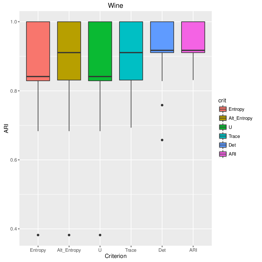
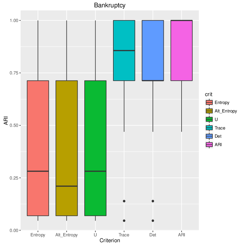
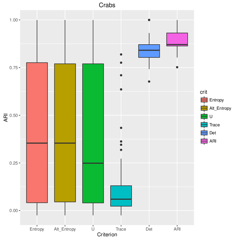
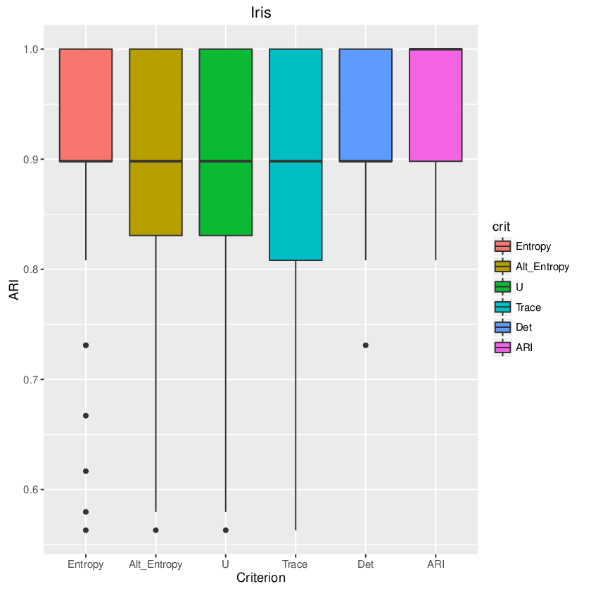
The distributions of the ARI values for the three classification-based criteria show that the resulting ARI from the chosen weight is generally much lower than if we were to use the highest ARI. Moreover, the variability is generally much higher and especially so for the bankruptcy and crabs data. On the other hand, performs well in comparison to the three classification-based criteria for the wine and bankruptcy data. Furthermore, in the case of the bankruptcy data, it performs the best of all five criteria, when comparing the medians, and has a distribution closest to that of the highest ARI. However, in the case of the crabs data, it performs very poorly, and has the worst performance of the five criteria. For the iris data, the performance is similar to the alternative entropy and criteria. Finally, we see that performs well for all of the datasets. In the case of the wine data, except for a couple of outliers, the distribution is very similar to that for the highest ARI — this is quite remarkable when one considers that the ARI assumes knowledge of the true labels. Furthermore, performs the best of all of the proposed criteria in all of the datasets except for the bankruptcy data. In this case, performs better, but the inter-quartile ranges are very similar. Therefore, we propose as a criterion to select the weight in FSC.
The Determinant as a Model Selection Criterion
We have already seen that appears to be an effective selection criterion for the weight in FSC. Now, we consider the possibility of using this criterion for model selection in general. To further explore this idea, we once again consider the four datasets and perform 50 random splits with 80% of the data points having known labels. This time, we consider two different procedures. In the first procedure, we proceed as before and choose the model based on the BIC, and then the weight using . In the second, we choose the model based on and then the weight also based on . We once again take the ARI values after choosing the model and the weight using one of these two procedures, and we take the maximum ARI value amongst all of the weights. In Figure 14, we show box plots of the distributions of the ARI values. In (a) we show the results for the first procedure and, in (b), we show the results for the second procedure.
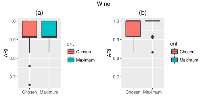
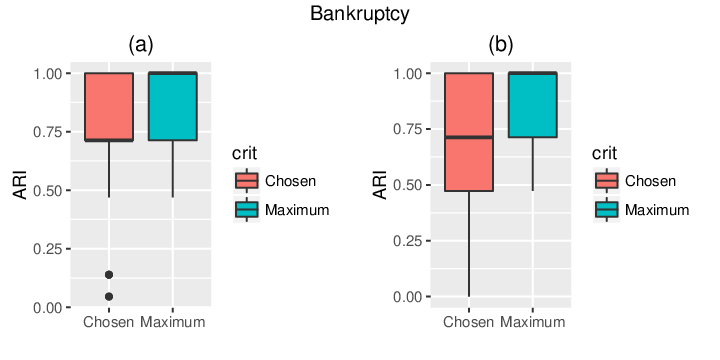

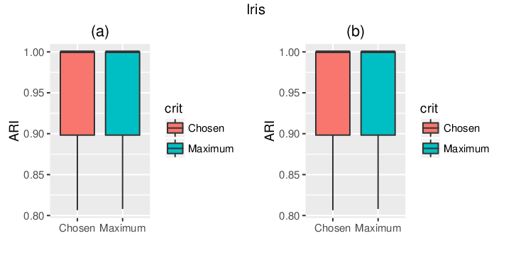
There are a few interesting items to note. First, for the wine dataset, we see that when using to choose the model, the distribution of the maximum ARI has a lot less variability. Also, these maximum ARI values are generally larger after using to choose the model. One final note on the wine dataset is that the median ARI values using procedure 2 is higher than those from procedure 1. For the bankruptcy data, we see that the distribution of the maximum ARI is the same regardless of using the BIC or to choose the model. However, after choosing the weight, we see that the distribution of the ARI values for procedure 2 shows more variability than procedure 1. In the case of the crabs data, we see that the distribution of the ARI for the selected model and weight are approximately the same for both procedures; however, the maximum ARI is generally better when using the BIC to choose the model. Finally, for the Iris data, all of the distributions are very similar. The results are inconclusive in that neither procedure outperformed the other; however, the fact that the BIC did not outperform for model selection is remarkable. In fact, the possibility of using for model selection in model-based clustering, as alternative to the BIC, is worthy of further consideration.
5.6 Justification for a Cluster Analysis
If some of the points are labelled, it may not be immediately clear as to why a cluster analysis should even be considered. However, there are situations in which performing a cluster analysis is just as good, if not better, than putting more weight on the labelled observations. In Figure 15, we show two different situations where this would be the case. In Table 2, we look at the ARI and for each of the weights for the two different cases. In the first case, only 10% of the points are labelled, and all labelled points are around the intersection of the two clusters. In this case, we see from the ARI and determinant values that we would only want give very little weight, or no weight, to the labelled observations.

| First Case | Second Case | |||||
|---|---|---|---|---|---|---|
| Weight | ARI | Det. | ARI | Det. | ||
| 0 | 0.9341 | 81006 | 1 | 82849 | ||
| 0.1 | 0.9341 | 81006 | 1 | 82849 | ||
| 0.2 | 0.9341 | 81006 | 1 | 82849 | ||
| 0.3 | 0.9126 | 81984 | 1 | 82849 | ||
| 0.4 | 0.9126 | 81984 | 1 | 82849 | ||
| 0.5 | 0.9126 | 81984 | 1 | 82849 | ||
| 0.6 | 0.8914 | 84250 | 1 | 82849 | ||
| 0.7 | 0.8914 | 84250 | 1 | 82849 | ||
| 0.8 | 0.8914 | 84250 | 1 | 82849 | ||
| 0.9 | 0.0075 | 178858 | 1 | 82849 | ||
| 1 | 187192 | 1 | 82849 | |||
In the first case, we see that a cluster analysis is actually better than using higher weights, and just as good as using smaller weights. In the second case, 90% of the points are labelled, and the unlabelled points lie on the outside of the two clusters. From the ARI and values (Table 2), it is clear that all weights give perfect classification, including a cluster analysis, and thus a cluster analysis would perform just as well as the other weights in this case.
6 Conclusions and Future Work
The major contribution of this paper is to encourage the use of as a weight selection criterion in FSC. Although based on old ideas, and ideas that have not been fashionable for some time, this criteria is shown to outperform alternatives such as the near-ubiquitous BIC for weight selection. Furthermore, it performs comparably to the BIC in the model selection stage. As a secondary contribution, the FSC approach is shown to be mathematically tractable and effective for mixtures of multivariate -distributions. For example, in our simulations, the selected weight very rarely corresponded to one of the three traditional species of classification. Furthermore, in our real data analyses, the use of a mixture of multivariate -distributions was shown to either perform as well as or, in the case of the wine and bankruptcy datasets, better than the mixture of multivariate Gaussian distributions. This is likely due, at least in part, to the -distribution being more robust to outliers than the Gaussian distribution. It is not unreasonable to expect that the FSC will also perform well with other non-Gaussian mixtures — the reader is referred to the recent review paper of McNicholas (2016b) for some discussion of non-Gaussian mixtures.
Future work will investigate using as an alternative to the BIC for model selection in model-based clustering and classification in general. Using the FSC approach in a wider range of situations will also be explored. For example, FSC could be applied in the area of item response theory.
Acknowledgements
This work is supported by a Vanier CGS-D scholarship from the Natural Sciences and Engineering Research Council of Canada (Gallaugher) and the Canada Research Chairs program (McNicholas).
References
- Aitken (1926) Aitken, A. C. (1926). A series formula for the roots of algebraic and transcendental equations. Proceedings of the Royal Society of Edinburgh 45, 14–22.
- Andrews and McNicholas (2011a) Andrews, J. L. and P. D. McNicholas (2011a). Extending mixtures of multivariate t-factor analyzers. Statistics and Computing 21(3), 361–373.
- Andrews and McNicholas (2011b) Andrews, J. L. and P. D. McNicholas (2011b). Mixtures of modified t-factor analyzers for model-based clustering, classification, and discriminant analysis. Journal of Statistical Planning and Inference 141(4), 1479–1486.
- Andrews and McNicholas (2012) Andrews, J. L. and P. D. McNicholas (2012). Model-based clustering, classification, and discriminant analysis via mixtures of multivariate -distributions: The EIGEN family. Statistics and Computing 22(5), 1021–1029.
- Andrews and McNicholas (2014) Andrews, J. L. and P. D. McNicholas (2014). Variable selection for clustering and classification. Journal of Classification 31(2), 136–153.
- Andrews et al. (2016) Andrews, J. L., J. R. Wickins, N. M. Boers, and P. D. McNicholas (2016). teigen: Model-Based Clustering and Classification with the Multivariate t Distribution. R package version 2.2.0.
- Banfield and Raftery (1993) Banfield, J. D. and A. E. Raftery (1993). Model-based Gaussian and non-Gaussian clustering. Biometrics 49(3), 803–821.
- Baum et al. (1970) Baum, L. E., T. Petrie, G. Soules, and N. Weiss (1970). A maximization technique occurring in the statistical analysis of probabilistic functions of Markov chains. Annals of Mathematical Statistics 41, 164–171.
- Bensmail et al. (1997) Bensmail, H., G. Celeux, A. Raftery, and C. Robert (1997). Inference in model-based cluster analysis. Statistics and Computing 7, 1–10.
- Biernacki et al. (2000) Biernacki, C., G. Celeux, and G. Govaert (2000). Assessing a mixture model for clustering with the integrated completed likelihood. IEEE Transactions on Pattern Analysis and Machine Intelligence 22(7), 719–725.
- Celeux and Govaert (1995) Celeux, G. and G. Govaert (1995). Gaussian parsimonious clustering models. Pattern Recognition 28(5), 781–793.
- Celeux and Soromenho (1996) Celeux, G. and G. Soromenho (1996). An entropy criterion for assessing the number of clusters in a mixture model. Journal of Classification 13, 195–212.
- Dang et al. (2015) Dang, U. J., R. P. Browne, and P. D. McNicholas (2015). Mixtures of multivariate power exponential distributions. Biometrics 71(4), 1081–1089.
- Dempster et al. (1977) Dempster, A. P., N. M. Laird, and D. B. Rubin (1977). Maximum likelihood from incomplete data via the EM algorithm. Journal of the Royal Statistical Society: Series B 39(1), 1–38.
- Edwards and Cavalli-Sforza (1965) Edwards, A. W. F. and L. L. Cavalli-Sforza (1965). A method for cluster analysis. Biometrics 21, 362–375.
- Fraley and Raftery (1998) Fraley, C. and A. E. Raftery (1998). How many clusters? Which clustering methods? Answers via model-based cluster analysis. The Computer Journal 41(8), 578–588.
- Franczak et al. (2014) Franczak, B. C., R. P. Browne, and P. D. McNicholas (2014). Mixtures of shifted asymmetric Laplace distributions. IEEE Transactions on Pattern Analysis and Machine Intelligence 36(6), 1149–1157.
- Franczak et al. (2015) Franczak, B. C., C. Tortora, R. P. Browne, and P. D. McNicholas (2015). Unsupervised learning via mixtures of skewed distributions with hypercube contours. Pattern Recognition Letters 58(1), 69–76.
- Friedman and Rubin (1967) Friedman, H. P. and J. Rubin (1967). On some invariant criteria for grouping data. Journal of the American Statistical Association 62, 1159–1178.
- Gordon (1981) Gordon, A. D. (1981). Classification. London: Chapman and Hall.
- Hubert and Arabie (1985) Hubert, L. and P. Arabie (1985). Comparing partitions. Journal of Classification 2(1), 193–218.
- Hurley (2004) Hurley, C. (2004). Clustering visualizations of multivariate data. Journal of Computational and Graphical Statistics 13(4), 788–806.
- Ingrassia et al. (2015) Ingrassia, S., S. C. Minotti, A. Punzo, and G. Vittadini (2015). The generalized linear mixed cluster-weighted model. Journal of Classification 32(1), 85–113.
- Ingrassia et al. (2012) Ingrassia, S., S. C. Minotti, and G. Vittadini (2012). Local statistical modeling via the cluster-weighted approach with elliptical distributions. Journal of Classification 29(3), 363–401.
- Lee and McLachlan (2014) Lee, S. and G. J. McLachlan (2014). Finite mixtures of multivariate skew t-distributions: some recent and new results. Statistics and Computing 24, 181–202.
- Lee and McLachlan (2013) Lee, S. X. and G. J. McLachlan (2013). On mixtures of skew normal and skew t-distributions. Advances in Data Analysis and Classification 7(3), 241–266.
- Lin (2010) Lin, T.-I. (2010). Robust mixture modeling using multivariate skew t distributions. Statistics and Computing 20(3), 343–356.
- Lin et al. (2016) Lin, T.-I., G. J. McLachlan, and S. X. Lee (2016). Extending mixtures of factor models using the restricted multivariate skew-normal distribution. Journal of Multivariate Analysis 143, 398–413.
- Lin et al. (2014) Lin, T.-I., P. D. McNicholas, and J. H. Hsiu (2014). Capturing patterns via parsimonious t mixture models. Statistics and Probability Letters 88, 80–87.
- MacQueen (1967) MacQueen, J. (1967). Some methods for classification and analysis of multivariate observations. In Proceedings of the Fifth Berkeley Symposium on Mathematical Statistics and Probability, Volume 1: Statistics, Berkeley, pp. 281–297. University of California Press.
- McNicholas (2016a) McNicholas, P. D. (2016a). Mixture Model-Based Classification. Boca Raton: Chapman & Hall/CRC Press.
- McNicholas (2016b) McNicholas, P. D. (2016b). Model-based clustering. Journal of Classification 33(3), 331–373.
- McNicholas and Murphy (2008) McNicholas, P. D. and T. B. Murphy (2008). Parsimonious Gaussian mixture models. Statistics and Computing 18(3), 285–296.
- McNicholas et al. (2010) McNicholas, P. D., T. B. Murphy, A. F. McDaid, and D. Frost (2010). Serial and parallel implementations of model-based clustering via parsimonious Gaussian mixture models. Computational Statistics and Data Analysis 54(3), 711–723.
- Murray et al. (2014a) Murray, P. M., R. B. Browne, and P. D. McNicholas (2014a). Mixtures of skew-t factor analyzers. Computational Statistics and Data Analysis 77, 326–335.
- Murray et al. (2017a) Murray, P. M., R. B. Browne, and P. D. McNicholas (2017a). Hidden truncation hyperbolic distributions, finite mixtures thereof, and their application for clustering. Journal of Multivariate Analysis 161, 141–156.
- Murray et al. (2017b) Murray, P. M., R. B. Browne, and P. D. McNicholas (2017b). A mixture of SDB skew-t factor analyzers. Econometrics and Statistics 3, 160–168.
- Murray et al. (2014b) Murray, P. M., P. D. McNicholas, and R. B. Browne (2014b). A mixture of common skew- factor analyzers. Stat 3(1), 68–82.
- Orchard and Woodbury (1972) Orchard, T. and M. A. Woodbury (1972). A missing information principle: Theory and applications. In L. M. Le Cam, J. Neyman, and E. L. Scott (Eds.), Proceedings of the Sixth Berkeley Symposium on Mathematical Statistics and Probability, Volume 1: Theory of Statistics, pp. 697–715. Berkeley: University of California Press.
- Peel and McLachlan (2000) Peel, D. and G. J. McLachlan (2000). Robust mixture modelling using the t distribution. Statistics and Computing 10(4), 339–348.
- Punzo and McNicholas (2017) Punzo, A. and P. D. McNicholas (2017). Robust clustering in regression analysis via the contaminated Gaussian cluster-weighted model. Journal of Classification 34(2), 249–293.
- R Core Team (2016) R Core Team (2016). R: A Language and Environment for Statistical Computing. Vienna, Austria: R Foundation for Statistical Computing.
- Schwarz (1978) Schwarz, G. (1978). Estimating the dimension of a model. The Annals of Statistics 6(2), 461–464.
- Scott and Symons (1971) Scott, A. J. and M. J. Symons (1971). Clustering methods based on likelihood ratio criteria. Biometrics 27, 387–397.
- Steane et al. (2012) Steane, M. A., P. D. McNicholas, and R. Yada (2012). Model-based classification via mixtures of multivariate t-factor analyzers. Communications in Statistics – Simulation and Computation 41(4), 510–523.
- Subedi et al. (2013) Subedi, S., A. Punzo, S. Ingrassia, and P. D. McNicholas (2013). Clustering and classification via cluster-weighted factor analyzers. Advances in Data Analysis and Classification 7(1), 5–40.
- Subedi et al. (2015) Subedi, S., A. Punzo, S. Ingrassia, and P. D. McNicholas (2015). Cluster-weighted t-factor analyzers for robust model-based clustering and dimension reduction. Statistical Methods and Applications 24(4), 623–649.
- Tiedeman (1955) Tiedeman, D. V. (1955). On the study of types. In S. B. Sells (Ed.), Symposium on Pattern Analysis. Randolph Field, Texas: Air University, U.S.A.F. School of Aviation Medicine.
- Tortora et al. (2015) Tortora, C., R. P. Browne, B. C. Franczak, and P. D. McNicholas (2015). MixGHD: Model Based Clustering, Classification and Discriminant Analysis Using the Mixture of Generalized Hyperbolic Distributions. R package version 1.8.
- Venables and Ripley (2002) Venables, W. N. and B. D. Ripley (2002). Modern Applied Statistics with S (Fourth ed.). New York: Springer. ISBN 0-387-95457-0.
- Vrbik and McNicholas (2012) Vrbik, I. and P. D. McNicholas (2012). Analytic calculations for the EM algorithm for multivariate skew-t mixture models. Statistics and Probability Letters 82(6), 1169–1174.
- Vrbik and McNicholas (2014) Vrbik, I. and P. D. McNicholas (2014). Parsimonious skew mixture models for model-based clustering and classification. Computational Statistics and Data Analysis 71, 196–210.
- Vrbik and McNicholas (2015) Vrbik, I. and P. D. McNicholas (2015). Fractionally-supervised classification. Journal of Classification 32(3), 359–381.
- Wolfe (1965) Wolfe, J. H. (1965). A computer program for the maximum likelihood analysis of types. Technical Bulletin 65-15, U.S. Naval Personnel Research Activity.
Appendix A tEIGEN Models
| Model | No. of Free Covariance Parameters | ||||
|---|---|---|---|---|---|
| CIIC | C | I | I | C | 1+1 |
| CIIU | C | I | I | U | |
| UIIC | U | I | I | C | |
| UIIU | U | I | I | U | |
| CICC | C | I | C | C | |
| CICU | C | I | C | U | |
| UICC | U | U | C | C | |
| UICU | U | I | C | U | |
| CIUC | C | I | U | C | |
| CIUU | C | I | U | U | |
| UIUC | U | I | U | C | |
| UIUU | U | I | U | U | |
| CCCC | C | C | C | C | [ |
| CCCU | C | C | C | U | [ |
| UCCC | U | C | C | C | [ |
| UCCU | U | C | C | U | [ |
| CUCC | C | U | C | C | |
| CUCU | C | U | C | U | |
| UUCC | U | U | C | C | |
| UUCU | U | U | C | U | |
| CCUC | C | C | U | C | [ |
| CCUU | C | C | U | U | [ |
| CUUC | C | U | U | C | |
| CUUU | C | U | U | U | |
| UCUC | U | C | U | C | |
| UCUU | U | C | U | U | |
| UUUC | U | U | U | C | |
| UUUU | U | U | U | U |
Appendix B Alternative Form of the Likelihood
B.1 Alternative Likelihood
We have already seen that the observed weighted likelihood can be written as in (5) and, analogous to (6), the associated complete-data weighted likelihood can be written as
| (15) |
Dempster et al. (1977) state that when integrating the complete-data likelihood over the space of unknown quantities, in our case , it is desired that the result should be the observed likelihood. The observed likelihood as given in (5), however, does not satisfy this property. Indeed,
| (16) |
where
Clearly, this is not the same as the form given in (5). Therefore, to maintain the relationship between the complete and incomplete weighted likelihood as presented in Dempster et al. (1977), we consider using the form of the incomplete weighted likelihood given in (16) and denote this by .
Note that there are two extreme cases that should be considered separately. The first extreme case is when :
which is equivalent to (16) when . The second extreme case, which turns out to be more interesting, is when :
which is the same as , the observed likelihood for a discriminant analysis. However, in (16), when ,
| (17) |
When we are performing a discriminant analysis and so the form of the observed and weighted likelihoods should be the same, which is clearly not the case. Therefore, when , we use for our observed likelihood.
For both the original and altered observed likelihoods, the complete-data likelihood is identical. Therefore, if we were to take a Gaussian mixture model, the updates in the M-step would be the same as those given in Vrbik and McNicholas (2015), regardless of whether the original or alternative likelihood were used. However, the updates for in the E-step would become
B.2 Simulation Comparing the Original and Altered Likelihoods
We perform simulations to compare the performance of the original and altered likelihoods. We simulate 100 datasets with 300 samples: 150 of these sample belong to one group which follows a , and the remaining 150 belong to another group which follows a , where and
We take corresponding to different levels of clustering difficulty. For each dataset, we consider , where is the percentage of labelled data.
To choose the weights for FSC, we looked at 11 different values of . These values were taken to be , where . We then calculate the ARI for each of these weights for the 100 datasets and take the average ARI for each weight. We then choose the weight that had the highest average ARI. We denote the resulting FSC solution for each weight by FSC. Furthermore, denote by FSCARI the FSC solution with the chosen weight resulting from the highest average ARI. Finally, in the special cases corresponding to the three species of classification , we denote the FSC solution by FSCclust, FSCclass and FSCDA, respectively.
In Figures 16 and 17, we show different line plots for and , respectively. In each plot, the average ARI is plotted against the percentage of labelled data . A dotted black line is used to show the result for FSCARI with the corresponding chosen weight shown above each point. The first row in each plot shows the results when using all the weights, and the second row singles out the three different species of classification and FSCARI The standard errors were calculated by taking the ARI for all 100 datasets of the chosen weight of FSCARI and calculating one (darker grey) and two (lighter grey) standard deviations from the mean ARI.


In general, the overall classification performance between the altered and original likelihoods are similar. The chosen weights for FSCARI, however, differ between the two forms of the likelihood. For , this difference is less pronounced than for . More specifically, for , the difference between the weights for all but 10%, 30% and 50% differ by at most 0.1 if they are not exactly the same. For , however, the differences between the chosen weights are greater, and there are fewer proportions for which the difference is small. We also see that at lower percentages of labelled data, there is more variability in the average ARI between the different weights. In conclusion, although the choice of the weights are different between the two likelihoods, the overall classification performance when using the chosen weight in each case are very similar. Moreover, the altered form is not strictly a likelihood. Accordingly, we will henceforth use the original, and more natural form, form of the likelihood for FSC.