Exact computation of a manifold metric, via Lipschitz Embeddings and Shortest Paths on a Graph

Timothy Chu^* Affiliation: CMU Email: timothyzchu@gmail.com Gary L. Miller ^†^†thanks: Partially supported by NSF CCF-1637523 Affiliation: CMU Email: glmiller@cs.cmu.edu
Donald R. Sheehy ^†^†thanks: Partially supported by NSF CCF-1652218 Affiliation: North Carolina State University Email: don.r.sheehy@gmail.com

Abstract

Data-sensitive metrics adapt distances locally based the density of data points with the goal of aligning distances and some notion of similarity. In this paper, we give the first exact algorithm for computing a data-sensitive metric called the nearest neighbor metric. In fact, we prove the surprising result that a previously published $3$ -approximation is an exact algorithm.

The nearest neighbor metric can be viewed as a special case of a density-based distance used in machine learning, or it can be seen as an example of a manifold metric. Previous computational research on such metrics despaired of computing exact distances on account of the apparent difficulty of minimizing over all continuous paths between a pair of points.

We leverage the exact computation of the nearest neighbor metric to compute sparse spanners and persistent homology. We also explore the behavior of the metric built from point sets drawn from an underlying distribution and consider the more general case of inputs that are finite collections of path-connected compact sets.

The main results connect several classical theories such as the conformal change of Riemannian metrics, the theory of positive definite functions of Schoenberg, and screw function theory of Schoenberg and Von Neumann. We also develop some novel proof techniques based on the combination of screw functions and Lipschitz extensions that may be of independent interest.

1 Introduction

The profound success of nonlinear methods in machine learning such as kernels methods, density-based distances, and neural nets reveals that although data are often represented as points in $\mathbb{R}^{n}$ , the shortest path between two points is not a straight line. It is widely believed that a more useful metric on the data points would have the property that two points in a dense cluster will be close in some underlying metric, even if the Euclidean distance is far [AvL12, CFM+15, VB03, BRS11]. That is, distances are scaled inversely according to the density of the data along a path between points. We call such a metric data-sensitive.

Data-sensitive metrics arise naturally in machine learning, and are implicitly central in celebrated methods such as $k$ -NN graph methods, manifold learning, level-set methods, single-linkage clustering, and Euclidean MST-based clustering (see Section 5 and Appendix A for details). The construction of appropriate data-sensitive metrics is an active area of research. We consider a simple data-sensitive metric with an underlying manifold structure called the nearest neighbor metric. This metric was first introduced in [CFM+15]. It and its close variants have been studied in the past by multiple researchers [HDHI16, CFM+15, SO05, BRS11, VB03]. In this paper, we show how to compute the nearest neighbor metric exactly for any dimension, which solves one of the most important and challenging problems for any manifold-based metric.

The starting point will be the nearest neighbor function $\mathbf{r}_{P}$ for the data set $P$ :

\mathbf{r}_{P}(z)=4\min_{x\in p}\|x-z\|,

where the factor of $4$ normalizes and simplifies expressions later. This function is also known as the distance function to the set $P$ and is the basic object of study in the critical point theory of distance functions, a generalization of Morse Theory [Gro93]. This theory has found many recent uses in computational geometry [CL08, CCSL09] as it is a natural way to infer underlying structure from a sample of points. We have a similar goal of inferring underlying structure when we use $\mathbf{r}_{P}$ as a cost function for a density-based distance defined as follows (see also Section 4 for explicit inference results).

Definition 1.1

Given a continuous cost function $c:\mathbb{R}^{k}\rightarrow\mathbb{R}$ , we define the density-based cost of a path $\gamma$ relative to $c$ as:

\ell_{c}(\gamma)=\int_{0}^{1}c(\gamma(t))\|\gamma^{\prime}(t)\|dt.

Here, the path $\gamma$ is defined as a continuous map $\gamma:[0,1]\to\mathbb{R}^{k}$ . Let $\mathrm{path}(a,b)$ denote the set of piecewise- $C_{1}$ paths from $a$ to $b$ . We then define the density-based distance between two points $a,b\in\mathbb{R}^{k}$ as

d_{c}(a,b)\inf_{\gamma\in\mathrm{path}(a,b)}\ell_{c}(\gamma)

This is a slight simplification of the density-based distances from [SO05] which included other requirements to facilitate approximation. Conceptually, the density-based cost of a path is the weighted path length, where each infinitesimal path piece is weighted according to $c$ . The cost $c$ is usually some function of an underlying density $f$ (the natural choice would be $c(x)=f(x)^{-\frac{1}{k}}$ ). Density-based distances have been notable in the machine learning setting for over a decade [SO05, BRS11]. To build a data-sensitive metric from density-based distances, we would like a cost function $c$ that is small when close to the data set, and large when far away. The nearest neighbor function $\mathbf{r}_{P}$ is the most natural candidate, and has been traditionally used as a proximity measure between points and a data set in both the geometry and machine learning settings [BRS11]. It has been used as such in nearest neighbor (and $k$ -NN) classification, $k$ -means/medians/center clustering, finite element methods, and any of the numerous methods that use Voronoi diagrams or Delaunay triangulation as intermediate data structures.

Definition 1.2

Given any finite set $P\subset\mathbb{R}^{k}$ , the nearest neighbor cost function is $\ell_{N}:=\ell_{\mathbf{r}_{P}}$ and the nearest neighbor metric is $\mathbf{d}_{N}:=\mathbf{d}_{\mathbf{r}_{P}}$ . That is, it’s the density-based distance with cost function $\mathbf{r}_{P}$ .

Refer to caption — Figure 1: In this figure we have a collection of points. The length or cost of the green curve between the two blue points is the integral along the curve scaled by the distance to the nearest point.

The nearest neighbor metric, and density-based distances in general, are examples of manifold geodesics [SO05, TdSL00]. Manifold geodesics of data sets are defined by embedding points into a manifold and computing the infimum length path in the manifold. Within computer science, dozens of foundational papers in machine learning and surface reconstruction rely on manifold-based metrics to perform clustering, classification, regression, surface reconstruction, persistent homology, and more [TdSL00, CFM+15, VB03, BRS11, SO05, ELZ02, AvL12, Lux07]. Manifold geodesics predate computer science, and are the cornerstone of many fields of physics and mathematics. Exactly computing geodesics is fundamental to countless areas of physics including: the brachistochrone and minimal-drag-bullet problem of Bernoulli and Newton [Ber96], exactly determining a particle’s trajectory in classical physics (Hamilton’s Principle of Least Action) [CH53], computing the path of light through a non-homogeneous medium (Snell’s law), finding the evolution of wave functions in quantum mechanics over time (Feynman path integrals [Fey48]), and determining the path of light in the presence of gravitational fields (General Relativity, Schwarzschild metric) [Sch16, SW97]. In mathematics, manifold geodesics appear in many branches of higher mathematics including differential equations, differential geometry, Lie theory, calculus of variations, algebraic geometry, and topology.

One of the most significant problems on any manifold geodesic is how to compute its length. Exact computation of manifold metrics is considered a fundamental problem in mathematics and physics, dating back for four centuries: entire fields of mathematics, including the celebrated calculus of variations, have arisen to tackle this [CH53]. Historically, mathematicians placed strong emphasis on exact computation as opposed to constant factor approximations [CH53]. An algorithmic problem on manifold geodesics, with modern origins, is to $(1+\varepsilon)$ approximate these metrics efficiently on a computer. The core difficulty in the first problem is that geodesics are the minimum cost path out of an uncountable number of paths that can travel ’anywhere’ on the manifold structure. This makes exactly computing these metrics challenging, even in the case of the nearest neighbor metric for just four fixed points in two dimensions (the authors are unaware of any easy method for this simplified task). Calculus of variations can show that the optimal nearest neighbor path is piecewise hyperbolic, but this is generally insufficient to exactly compute the nearest neighbor metric—there are point sets where there are many differentiable, piecewise hyperbolic paths between two data points with different costs.

In this paper, we solve both problems: we exactly compute the Nearest Neighbor metric in all cases, and we $(1+\varepsilon)$ approximate it quickly. Our approach is based on a novel embedding of the data into high dimensions where the geodesics are straight lines. Then we use a Lipschitz extension theorem to relate the lengths of the shortest paths in the original space and the embedding. We combine these tools to prove that the nearest neighbor metric is exactly equal to a shortest path distance on a geometric graph, the so-called edge-squared metric, in all cases. This allows us to compute the nearest-neighbor metric exactly for any given point set in polynomial time, and it is the only known (non-trivial) density-based distance that can be computed by a discrete algorithm.

Definition 1.3

For $x\in\mathbb{R}^{d}$ , let $\|x\|$ denote the Euclidean norm. For a set of points $P\subset\mathbb{R}^{d}$ : the edge-squared metric for $a,b\in P$ is

\mathbf{d}_{2}(a,b)=\inf_{(p_{0},\ldots,p_{k})}\sum_{i=1}^{k}\|p_{i}-p_{i-1}\|^{2},

where the infimum is over sequences of points $p_{0},\ldots,p_{k}\in P$ with $p_{0}=a$ and $p_{k}=b$ .

Theorem 1.1

The nearest neighbor metric and edge squared metric are equivalent for any set $P$ in arbitrary dimension that is the finite collection of compact path-connected sets.

This in particular covers the case of $n$ points in $n-1$ dimension. The exact equality is realized when the nearest neighbor path is piecewise linear, traveling straight from data point to data point. The edge squared metric has been previously studied by multiple researchers in machine learning and power-efficient wireless networks, but previously has only been linked to the nearest neighbor metric by a fairly weak 3-approximation [CFM+15]. There are several reasons why it is surprising that these metrics are equal:

1.

The optimal nearest neighbor path for two points not in the dataset is generally composed of hyperbolic arcs. This holds true even when the dataset is a single point, and was established by [CFM+15] using tools in Riemannian surfaces and the complex plane. Meanwhile, our Theorem implies an optimal nearest neighbor path for two data points (in a dataset of any size) is piecewise linear!
2.

There are simple and natural variants of the nearest neighbor metric, for which no analog of Theorem 1.1 is known nor suspected. For example, if one considers powers (other than one) of the distance function as a cost, a corresponding graph-based metric is known to exist only for sets of size at most two.
3.

For just three points in a right triangle configuration, there exist an uncountable suite of optimal-cost paths between the two endpoints of the hypotenuse. Each path in this uncountable suite is piecewise hyperbolic, but, surprisingly, they all have the exact same cost as the edge-squared distance. Thus, there shortest paths may not even be unique.
4.

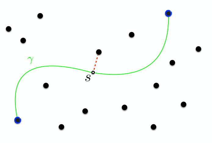
The finite union of compact path-connected geometric bodies in arbitrary dimension can have extremely complicated geometry, and the Voronoi diagram on which the nearest neighbor metric depends is poorly understood for even three of these bodies in two dimension. There is no other restriction on the compact geometric objects, and they need not be convex or even simply connected, see figure 2.

Figure 2: In this figure we have a collection of compact bodies in black. The length or cost of the green curve between the two blue points is the integral along the curve scaled by the distance to the nearest body. A curve may traverse a body at no cost. Theorem 1.1 establishes that the shortest path curve between two points goes straight from compact body to compact body.

We can now tackle a second problem of interest for manifold geodesics, which is efficiently $(1+\varepsilon)$ approximating them. In this paper, we show that the nearest neighbor metric admits $(1+\epsilon)$ spanners computable in nearly-linear time, with linear size, for any point set in constant dimension. Remarkably, these spanners are significantly sparser and faster to compute than the theoretically optimal Euclidean spanners with the same approximation constant, and nearly match the sparsity of the best known Euclidean Steiner spanners. Moreover, if the point set comes from a well-behaved probability distribution in constant dimension (a foundational assumption in machine learning [HDHI16]), we show that the nearest neighbor metric has perfect $1$ -spanners of nearly linear size. The latter result is impossible for many non-density sensitive metrics, such as the Euclidean metric. Both results rely on Theorem 1.1, and significantly improve the nearest neighbor spanners of Cohen et al in [CFM+15].

Theorem 1.1 and our spanner theorems solve two core problems of interest for the nearest neighbor metric: exactly computing it for any dimension, and approximating it quickly for both general point sets and point sets arising from a well-behaved probability distribution in constant dimension. This is the first work we know of that computes a manifold metric exactly without calculus of variations, and we hope that our tools can be useful for other metric computations and approximations.

1.1 Contributions and Past Work

Our primary contribution is Theorem 1.1, which lets us exactly compute the nearest neighbor metric. This significantly strengthens a core result of Cohen et al [CFM+15]. This theorem should be considered quite surprising: it equates the nearest neighbor metric with the edge-squared metric, even when the point set is a collections of compact, path-connected objects in arbitrarily large dimension. There are no restrictions on the convexity or simple-connectedness of such objects, so in general the Voronoi diagram of these objects (on which the nearest neighbor metric critically depends) can be extremely complicated.

Besides for exactly computing the nearest neighbor metric, we present the following theorems on approximate computation:

Theorem 1.2

For any set of points in $\mathbb{R}^{d}$ for constant $d$ , there exists a $(1+\varepsilon)$ spanner of the nearest neighbor metric with size $O\left(n\varepsilon^{-d/2}\right)$ computable in time $O\left(n\log n+n\varepsilon^{-d/2}\log{\frac{1}{\varepsilon}}\right)$ . The $\log{\frac{1}{\varepsilon}}$ term goes away given access to an algorithm computing floor function in $O(1)$ time.

Theorem 1.3

Suppose points $P$ in Euclidean space are drawn i.i.d from a Lipschitz probability density bounded above and below by a constant, with support on a smooth, connected, compact manifold with intrinsic dimension $d$ with boundary of bounded curvature. Then w.h.p. the $k$ -NN graph of $P$ for $k=O(2^{d}\ln n)$ and edges weighted with Euclidean distance squared, is a $1$ -spanner of the nearest neighbor metric on $P$ .

These theorems rely on Theorem 1.1 and considerably strengthen the spanner results on the nearest neighbor metric from [CFM+15]. They critically rely on Theorem 1.1, which show it suffices to compute spanners of the edge-squared metric. Previously, sparse spanners of the edge-squared metric were shown to exist in two dimensions via Yao graphs and Gabriel graphs [LWW01], but these did not generalize well to constant dimension: Yao graphs are not very efficient to compute, and Gabriel graphs can have quadratically many edges even in $3$ dimensions [CEG+94]. The spanners we produce are sparser than the theoretical optimal for Euclidean spanners [LS19].

Theorem 1.3 proves that a $1$ -spanner of the nearest neighbor metric can be found assuming points are samples from a probability density, by using a $k$ - $NN$ graph for appropriate $k$ . Our result is tight when $d$ is constant. This is not possible for Euclidean distance, as a $1$ -spanner is almost surely the complete graph. Although the restrictions on the probability density may seem limiting, they are in fact quite flexible and standard in machine learning theory and practice [HDHI16, AvL12]. For example, although they do not cover the case of a Gaussian (unbounded support), they do cover the case of a Gaussian where the very thin tail is cut off, and this recovers most of the relevant data in a Gaussian distribution. Past work on similar results include [BBSW05, GBQ03].

Theorem 1.1 will additionally allow us to compute the persistent homology of $\mathbf{d}_{N}$ , a task useful for topological data analysis [ELZ02]. We also show how the nearest neighbor metric generalizes Euclidean distance and maximum-edge Euclidean MST distance [LWW01]

The core mathematical contribution of our work is the statement and proof of Theorem 1.1. The techniques to prove our other results are simpler and mostly leverage Theorem 1.1 and past work. We have included them nonetheless to provide a more complete picture of the nearest neighbor metric, and to provide possible directions for future work.

1.2 Definitions and Preliminaries

In this section, we establish additional definitions for our paper. These are mostly of interest for our spanner and persistent homology results, and are not strictly necessary for Theorem 1.1.

Spanners: For real value $t\geq 1$ , a $t$ -spanner of a weighted graph $G$ is a subgraph $S$ such that $d_{G}(x,y)\leq d_{S}(x,y)\leq t\cdot d_{G}(x,y)$ where $d_{G}$ and $d_{S}$ represent the shortest path distance functions between vertex pairs in $G$ and $S$ . Spanners of Euclidean distances, and general graph distances, have been studied extensively, and their importance as a data structure is well established. [Che86, Vai91, CK93, HPIS13].

$k$ -nearest neighbor graphs: The $k$ -nearest neighbor graph ( $k$ -NN graph) for a set of objects $V$ is a graph with vertex set $V$ and an edge from $v\in V$ to its $k$ most similar objects in $V$ , under a given distance measure. In this paper, the underlying distance measure is Euclidean, and the edge weights are Euclidean distance squared. $k$ -NN graph constructions are a key data structure in machine learning [DCL11, CFS09], clustering [Lux07], and manifold learning [TdSL00].

Gabriel Graphs: The Gabriel graph is a graph where two vertices $p$ and $q$ are joined by an edge if and only if the disk with diameter $pq$ has no other points of $S$ in the interior. The Gabriel graph is a subgraph of the Delaunay triangulation [Sri15], and a $1$ -spanner of the edge-squared metric [Sri15]. Gabriel graphs will be used in the proof of Theorem 1.3.

Persistent Homology: Persistent homology is a popular tool in computational geometry and topology to ascribe quantitative topological invariants to spaces that are stable with respect to perturbation of the input. In particular, it’s possible to compare the so-called persistence diagram of a function defined on a sample to that of the complete space [CO08]. These two aspects of persistence theory—the intrinsic nature of topological invariants and the ability to rigorously compare the discrete and the continuous—are both also present in our theory of nearest neighbor metrics. Indeed, our primary motivation for studying these metrics was to use them as inputs to persistence computations for problems such as persistence-based clustering [CGOS13] or metric graph reconstruction [ACC+12].

2 Outline

Section 3 contains the proof of Theorem 1.1, equating the edge-squared metric and nearest neighbor metric in all cases. It should be noted that our proof is robust enough to handle not just finite point sets, but also countably infinite collections of disjoint path-connected, compact sets. Remarkably, there is no restriction on the convexity or simply-connectedness of these sets.

As an example of using the nearest neighbor metric to compute intrinsic structure, Section 4 shows how Theorem 1.1 allows us to compute the persistent homology of the nearest neighbor metric.

Section 5 introduces the $p$ -power metrics. We show that Euclidean spanners and Euclidean MSTs are special cases of $p$ -power spanners. We show how clustering algorithms including $k$ -means, level-set methods, and single linkage clustering, are special cases of clustering with $p$ -power metrics. $p$ -power metrics are identical to the Neighbor metric when $p=2$ . This is further detailed in Appendix A.

Section 6.2 outlines a proof of Theorem 1.2, and compares our spanner to new lower bounds on the sparsity of $(1+\varepsilon)$ -spanners of the Euclidean metric. We outline a proof of Theorem 1.3 in Section 6.1 and discuss its implications.

Conclusions and open questions are in Section 7. Full proofs for Theorems 1.3, 1.2 are contained in the Appendix.

3 Exactly Computing the nearest neighbor metric

In this section, we prove Theorem 1.1 on finite point sets, and explain in Section 3.1 that our proof strategy applies to finite collections of path-connected compact bodies.

First, lets observe what happens when $P$ has only two points $a$ and $b$ , $\mathbf{d}_{2}(a,b)=\mathbf{d}_{N}(a,b)$ . This reduces to a high school calculus exercise as the minimum path $\gamma$ will be a straight line between the points and the nearest neighbor metric is

	$\displaystyle\mathbf{d}_{N}(a,b)$	$\displaystyle=4\int_{0}^{1}\mathbf{r}_{P}(\gamma(t))\\|\gamma^{\prime}(t)\\|dt$
		$\displaystyle=8\int_{0}^{\frac{1}{2}}t\\|a-b\\|^{2}dt=\\|a-b\\|^{2}=\mathbf{d}_{2}(a,b).$

Now it is easy to observe that the nearest neighbor metric is never greater than the edge-squared distance, as proven in the following lemma.

Lemma 3.1

For all $s,p\in P$ , we have $\mathbf{d}_{N}(s,p)\leq\mathbf{d}_{2}(s,p)$ .

Fix any points $s,p\in P$ . Let $q_{0},\ldots,q_{k}\in P$ be such that $q_{0}=s$ , $q_{k}=p$ and

\mathbf{d}_{2}(s,p)=\sum_{i=1}^{k}\|q_{i}-q_{i-1}\|^{2}.

Let $\psi_{i}(t)=tq_{i}+(1-t)q_{i-1}$ be the straight line segment from $q_{i-1}$ to $q_{i}$ . Observe that $\ell(\psi_{i})=\|q_{i}-q_{i-1}\|^{2}/4$ , by the same argument as in the two point case. Then, let $\psi$ be the concatenation of the $\psi_{i}$ and it follows that

\mathbf{d}_{2}(s,p)=4\ell(\psi)\geq 4\inf_{\gamma\in\mathrm{path}(s,p)}\ell(\gamma)=\mathbf{d}_{N}(s,p).

By Lemma 3.1, it suffices to show that $\mathbf{d}_{N}(a,b)\geq\mathbf{d}_{2}(a,b)$ for all $a,b\in P$ .

Let $P\subset\mathbb{R}^{d}$ be a set of $n$ points. Pick any source point $s\in P$ . Order the points of $P$ as $p_{1},\ldots,p_{n}$ so that

\mathbf{d}_{2}(s,p_{1})\leq\cdots\leq\mathbf{d}_{2}(s,p_{n}).

This will imply that $p_{1}=s$ . It will suffice to show that for all $p_{i}\in P$ , we have $\mathbf{d}_{2}(s,p_{i})=\mathbf{d}_{N}(s,p_{i})$ . There are three main steps:

1.

We first show that when $P$ is a subset of the vertices of an axis-aligned box, $\mathbf{d}=\mathbf{d}_{N}$ . In this case, shortest paths for $\mathbf{d}$ are single edges and shortest paths for $\mathbf{d}_{N}$ are straight lines.
2.

We then show how to lift the points from $\mathbb{R}^{d}$ to $\mathbb{R}^{n}$ by a Lipschitz map $m$ that places all the points on the vertices of a box and preserves $\mathbf{d}_{2}(s,p)$ for all $p\in P$ .
3.

Finally, we show how the Lipschitz extension of $m$ is also Lipschitz as a function between nearest neighbor metrics. We combine these pieces to show that $\mathbf{d}\leq\mathbf{d}_{N}$ . As $\mathbf{d}\geq\mathbf{d}_{N}$ (Lemma 3.1), this will conclude the proof that $\mathbf{d}=\mathbf{d}_{N}$ .

The key to the second step, to be elaborated in Section 3.0.2, is that if you take points on a line and raise the pairwise distances to the $1/2$ power, you get points on a box. This is a special case of the general theory on screw functions developed by Von Neumann and Schoenberg, which asserts a far more general criterion on when functions applied to pairwise distances between points on a line can be embedded into Euclidean space [NS41].

3.0.1 Boxes

Let $Q$ be the vertices of a box in $\mathbb{R}^{n}$ . That is, there exist some positive real numbers $\alpha_{1},\ldots,\alpha_{n}$ such that each $q\in Q$ can be written as $q=\sum_{i\in I}\alpha_{i}e_{i}$ , for some $I\subseteq[n]$ .

Let the source $s$ be the origin. Let $\mathbf{r}_{Q}:\mathbb{R}^{n}\to\mathbb{R}$ be the distance function to the set $Q$ . Setting $r_{i}(x):=\min\{x_{i},\alpha_{i}-x_{i}\}$ (a lower bound on the difference in the $i$ th coordinate to a vertex of the box), it follows that

(3.1)

\mathbf{r}_{Q}(x)\geq\sqrt{\sum_{i=1}^{n}r_{i}(x)^{2}}.

Let $\gamma:[0,1]\to\mathbb{R}^{n}$ be a curve in $\mathbb{R}^{n}$ . Define $\gamma_{i}(t)$ to be the projection of $\gamma$ onto its $i$ th coordinate. Thus,

(3.2)

r_{i}(\gamma(t))=\min\{\gamma_{i}(t),\alpha_{i}-\gamma_{i}(t)\}

and

(3.3)

\|\gamma^{\prime}(t)\|=\sqrt{\sum_{i=1}^{n}\gamma_{i}^{\prime}(t)^{2}}.

We can bound the length of $\gamma$ as follows. For simplicity of exposition we only present the case of a path from the origin to the far corner, $p=\sum_{i=1}^{n}\alpha_{i}e_{i}$ .

	$\displaystyle\ell(\gamma)$	$\displaystyle=\int_{0}^{1}\mathbf{r}_{Q}(\gamma(t))\\|\gamma^{\prime}(t)\\|dt$
		[by definition]
		$\displaystyle\geq\int_{0}^{1}\left(\sqrt{\sum_{i=1}^{n}r_{i}(\gamma(t))^{2}}\sqrt{\sum_{i=1}^{n}\gamma_{i}^{\prime}(t)^{2}}\right)dt$
		[by (3.1) and (3.3)]
		$\displaystyle\geq\sum_{i=1}^{n}\int_{0}^{1}r_{i}(\gamma(t))\gamma_{i}^{\prime}(t)dt$
		[by Cauchy-Schwarz]
		$\displaystyle\geq\sum_{i=1}^{n}\left(\int_{0}^{\ell_{i}}\gamma_{i}(t)\gamma_{i}^{\prime}(t)dt+\int_{\ell_{i}^{\prime}}^{1}(\alpha_{i}-\gamma_{i}(t))\gamma_{i}^{\prime}(t)dt\right)$
		[by (3.2) where $\gamma_{i}(\ell_{i})=\alpha_{i}/2$ for the first time
		and $\gamma_{i}(\ell_{i}^{\prime})=\alpha_{i}/2$ for the last time.]
		$\displaystyle=\sum_{i=1}^{n}2\int_{0}^{\ell_{i}}\gamma_{i}(t)\gamma_{i}^{\prime}(t)dt$
		[by symmetry]
		$\displaystyle\geq\sum_{i=1}^{n}\frac{\alpha_{i}^{2}}{4}$
		[by basic calculus]

It follows that if $\gamma$ is any curve that starts at $s$ and ends at $p=\sum_{i=1}^{n}\alpha_{i}e_{i}$ , then $\mathbf{d}_{N}(s,p)=\mathbf{d}_{2}(s,p)$ .

3.0.2 Lifting the points to $\mathbb{R}^{n}$

Define a mapping $m:P\to\mathbb{R}^{n}$ . We do this by adding the points $p_{1},\ldots,p_{n}$ , as defined above, one point at a time. For each new point we will introduce a new dimension. We start by setting $m(p_{1})=0$ and by induction:

(3.4)

m(p_{i})=m(p_{i-1})+\sqrt{\mathbf{d}_{2}(s,p_{i})-\mathbf{d}_{2}(s,p_{i-1})}e_{i},

where the vectors $e_{i}$ are the standard basis vectors in $\mathbb{R}^{n}$ . A similar embedding works for some other functions and was extensively studied by Schoenberg and Von Neumann in the theory of screw functions.

Lemma 3.2

For all $p_{i},p_{j}\in P$ , we have

(i)

$\|m(p_{j})-m(p_{i})\|=\sqrt{|\mathbf{d}_{2}(s,p_{j})-\mathbf{d}_{2}(s,p_{i})|}$ , and
(ii)

$\|m(s)-m(p_{j})\|^{2}\leq\|m(p_{i})\|^{2}+\|m(p_{i})-m(p_{j})\|^{2}$ .

Proof of (i). Without loss of generality, let $i\leq j$ . Then, by the definition of $m$ , expanding the norm, and telescoping the sum, we get the following.

		$\displaystyle\\|m(p_{j})-m(p_{i})\\|$
		$\displaystyle=\left\\|\sum_{k=i+1}^{j}\sqrt{\mathbf{d}_{2}(s,p_{k})-\mathbf{d}_{2}(s,p_{k-1})}e_{k}\right\\|$
		$\displaystyle=\sqrt{\sum_{k=i+1}^{j}(\mathbf{d}_{2}(s,p_{k})-\mathbf{d}_{2}(s,p_{k-1}))}$
		$\displaystyle=\sqrt{\mathbf{d}_{2}(s,p_{j})-\mathbf{d}_{2}(s,p_{i})}.$

Proof of (ii). As $m(s)=0$ , it suffice to observe that

$\displaystyle\\|m(p_{j})\\|^{2}$	$\displaystyle=\mathbf{d}_{2}(s,p_{j})$	$\displaystyle\left[\text{\small{by \emph{(i)}}}\right]$
	$\displaystyle\leq\mathbf{d}_{2}(s,p_{i})+\|\mathbf{d}_{2}(s,p_{j})-\mathbf{d}_{2}(s,p_{i})\|$
	$\displaystyle=\\|m_{(}p_{i})\\|^{2}+\\|m(p_{i})-m(p_{j})\\|^{2}$	$\displaystyle\left[\text{\small{by \emph{(i)}}}\right]$

We can now show that $m$ has all of the desired properties.

Proposition 3.1

Let $P\subset\mathbb{R}^{d}$ be a set of $n$ points, let $s\in P$ be a designated source point, and let $m:P\to\mathbb{R}^{n}$ be the map defined as in (3.4). Let $\mathbf{d}^{\prime}$ denote the edge squared metric for the point set $m(P)$ in $\mathbb{R}^{n}$ . Then,

(i)

$m$ is $1$ -Lipschitz as a map between Euclidean metrics,
(ii)

$m$ maps the points of $P$ to the vertices of a box, and
(iii)

$m$ preserves the edge squared distance to $s$ , i.e. $\mathbf{d}^{\prime}(m(s),m(p))=\mathbf{d}_{2}(s,p)$ for all $p\in P$ .

Proof of (i). To prove the Lipschitz condition, fix any $a,b\in P$ and bound the distance as follows.

$\displaystyle\\|m(a)-m(b)\\|$	$\displaystyle=\sqrt{\|\mathbf{d}_{2}(s,a)-\mathbf{d}_{2}(s,b)\|}$	$\displaystyle\left[\text{\small{Lem.~\ref{lem:m_and_dist}(i)}}\right]$
	$\displaystyle\leq\sqrt{\mathbf{d}_{2}(a,b)}$	$\displaystyle\left[\text{\small{triangle ineq.}}\right]$
	$\displaystyle\leq\\|a-b\\|.$	$\displaystyle\left[\text{\small{by def. of $\mathbf{d}_{2}$}}\right]$

Proof of (ii). That $m$ maps $P$ to the vertices of a box is immediate from the definition. The box has side lengths $\|m_{i}-m_{i-1}\|$ for all $i>1$ and $p_{i}=\sum_{k=1}^{i}\|m_{k}-m_{k-1}\|e_{k}$ .

Proof of (iii). We can now show that the edge squared distance to $s$ is preserved. Let $q_{0},\ldots,q_{k}$ be the shortest sequence of points of $m(P)$ that realizes the edge-squared distance from $m(s)$ to $m(p)$ , i.e., $q_{0}=m(s)$ , $q_{k}=m(p)$ , and

\mathbf{d}^{\prime}(m(s),m(p))=\sum_{i=1}^{k}\|m(q_{i})-m(q_{i-1})\|^{2}.

If $k>1$ , then Lemma 3.2(ii) implies that removing $q_{1}$ gives a shorter sequence. Thus, we may assume $k=1$ and therefore, by Lemma 3.2(i),

\mathbf{d}^{\prime}(m(s),m(p))=\|m(s)-m(p)\|^{2}=\mathbf{d}_{2}(s,p).

3.0.3 The Lipschitz Extension

Proposition 3.1 and the Kirszbraun theorem on Lipschitz extensions imply that we can extend $m$ to a $1$ -Lipschitz function $f:\mathbb{R}^{d}\to\mathbb{R}^{n}$ such that $f(p)=m(p)$ for all $p\in P$ [Kir34, Val45, Bre81].

Lemma 3.3

The function $f$ is also $1$ -Lipschitz as mapping from $\mathbb{R}^{d}\to\mathbb{R}^{n}$ with both spaces endowed with the nearest neighbor metric.

We are interested in two distance functions $\mathbf{r}_{P}:\mathbb{R}^{d}\to\mathbb{R}$ and $\mathbf{r}_{f(P)}:\mathbb{R}^{n}\to\mathbb{R}$ . Recall that each is the distance to the nearest point in $P$ or $f(P)$ respectively.

$\displaystyle\mathbf{r}_{f(P)}(f(x))$	$\displaystyle=\min_{q\in f(P)}\\|q-f(x)\\|$	$\displaystyle\left[\text{\small{by definition}}\right]$
	$\displaystyle=\min_{p\in P}\\|f(p)-f(x)\\|$	$\displaystyle\left[\text{\small{$q\in f(P)$}}\right]$
	$\displaystyle\leq\min_{p\in P}\\|p-x\\|$	$\displaystyle\left[\text{\small{$f$ is $1$-Lipschitz}}\right]$
	$\displaystyle=\mathbf{r}_{P}(x).$	$\displaystyle\left[\text{\small{by definition}}\right]$

For any curve $\gamma:[0,1]\to\mathbb{R}^{d}$ and for all $t\in[0,1]$ , we have $\|(f\circ\gamma)^{\prime}(t)\|\leq\|\gamma^{\prime}(t)\|$ . It then follows that

	$\displaystyle\ell^{\prime}(f\circ\gamma)$	$\displaystyle=\int_{0}^{1}\mathbf{r}_{f(P)}(f(\gamma(t)))\\|(f\circ\gamma)^{\prime}(t)\\|dt$
(3.5)			$\displaystyle\leq\int_{0}^{1}\mathbf{r}_{P}(\gamma(t))\\|\gamma^{\prime}(t)\\|dt=\ell(\gamma),$

where $\ell^{\prime}$ denotes the length with respect to $\mathbf{r}_{f(P)}$ . Thus, for all $a,b\in P$ ,

$\displaystyle\mathbf{d}_{N}(a,b)$	$\displaystyle=4\inf_{\gamma\in\mathrm{path}(a,b)}\ell(\gamma)$	$\displaystyle\left[\text{\small{by definition}}\right]$
	$\displaystyle\geq 4\inf_{\gamma\in\mathrm{path}(a,b)}\ell^{\prime}(f\circ\gamma)$	$\displaystyle\left[\text{\small{by \eqref{eq:curves_shorten}}}\right]$
	$\displaystyle\geq 4\inf_{\gamma^{\prime}\in\mathrm{path}(f(a),f(b))}\ell^{\prime}(\gamma^{\prime})$	$\displaystyle\left[\text{\small{$f\circ\gamma$ is a path}}\right]$
	$\displaystyle=\mathbf{d}_{N}(f(a),f(b)).$	$\displaystyle\left[\text{\small{by definition}}\right]$

We now restate Theorem 1.1 for convenience, and prove it.

Theorem 3.1

For any point set $P\subset\mathbb{R}^{d}$ , the edge squared metric $\mathbf{d}$ and the nearest neighbor metric $\mathbf{d}_{N}$ are identical.

Fix any pair of points $s$ and $p$ in $P$ . Define the Lipschitz mapping $m$ and its extension $f$ as in (3.4). Let $\mathbf{d}^{\prime}$ and $\mathbf{d}_{N}^{\prime}$ denote the edge-squared and nearest neighbor metrics on $f(P)$ in $\mathbb{R}^{n}$ .

$\displaystyle\mathbf{d}_{2}(s,p)$	$\displaystyle=\mathbf{d}^{\prime}(m(s),m(p))$	$\displaystyle\left[\text{\small{Proposition~\ref{prop:m_is_good}(iii)}}\right]$
	$\displaystyle=\mathbf{d}_{N}^{\prime}(m(s),m(p))$	$\displaystyle\left[\text{\small{$f(P)$ are vertices of a box}}\right]$
	$\displaystyle\leq\mathbf{d}_{N}(s,p)$	$\displaystyle\left[\text{\small{Lemma~\ref{lem:dist_N_lipschitz}}}\right]$

We have just shown that $\mathbf{d}\leq\mathbf{d}_{N}$ and Lemma 3.1 states that $\mathbf{d}\geq\mathbf{d}_{N}$ , so we conclude that $\mathbf{d}=\mathbf{d}_{N}$ as desired.

3.1 From Finite Sets to Finite Collections of Compact Path-Connected Bodies

All of our proof steps hold for finite collections of compact, path-connected bodies in arbitrarily large dimension. Our Lipschitz map $m$ can still be extended to a Lipschitz map $f$ in this setting, largely due to the generality of the Kirszbraun theorem. In this case, the pre-image of the contractive map is the set of all points belonging to some body. Meanwhile, the image is a finite set of points, the corners of a multi-dimensional box. Thus our construction of $m$ contracts each convex body into a single point, and the image of our compact bodies under $f$ is still a finite point set on the corners of a box. Therefore, the remainder of our theorem proof goes through unchanged.

This result is rather remarkable: path-connected compact sets in high dimensional space can have extremely convoluted geometry, and the Voronoi diagrams on these collections (on which the nearest neighbor metric depends) can be massively complex. The key is that our Lipschitz map is robust enough to handle objects of considerable geometric complexity.

4 Persistent Homology of the Nearest-neighbor Geodesic Distance

In this section, we show how to compute the so-called persistent homology [ELZ02] of the nearest neighbor metric in two different ways, one ambient and the other intrinsic. The latter relies on Theorem 1.1 and would be quite surprising without it.

The input for persistence computation is a filtration—a nested sequence of spaces, usually parameterized by a real number $\alpha\geq 0$ . The output is a set of points in the plane called a persistence diagram that encodes the birth and death of topological features like connected components, holes, and voids.

The Ambient Persistent Homology

Perhaps the most popular filtration to consider on a Euclidean space is the sublevel set filtration of the distance to a sample $P$ . This filtration is $(F_{\alpha})_{\alpha\geq 0}$ , where

F_{\alpha}:=\{x\in\mathbb{R}^{d}\mid\mathbf{r}_{P}(x)\leq\alpha\},

for all $\alpha\geq 0$ . If one wanted to consider instead the nearest neighbor metric $\mathbf{d}_{N}$ , one gets instead a filtration $(G_{\alpha})_{\alpha\geq 0}$ , where

G_{\alpha}:=\{x\in\mathbb{R}^{d}\mid\min_{p\in P}\mathbf{d}_{N}(x,p)\leq\alpha\},

for all $\alpha\geq 0$ .

Both the filtrations $(F_{\alpha})$ and $(G_{\alpha})$ are unions of metric balls. In the former, they are Euclidean. In the latter, they are the metric balls of $\mathbf{d}_{N}$ . These balls can look very different, for example, for $\mathbf{d}_{N}$ , the metric balls are likely not even convex. However, these filtrations are very closely related.

Lemma 4.1

For all $\alpha\geq 0$ , $F_{\alpha}=G_{2\alpha^{2}}$ .

The key to this exercise is to observe that the nearest point $p\in P$ to a point $x$ is also the point that minimizes $\mathbf{d}_{N}(x,p)$ . To prove this, we will show that for any $p\in P$ and any path $\gamma\in\mathrm{path}(x,p)$ , we have $\ell(\gamma)\geq\frac{1}{2}\mathbf{r}_{P}(x)^{2}$ . Consider any such $x$ , $p$ , and $\gamma$ . The euclidean length of $\gamma$ must be at least $\mathbf{r}_{P}(x)$ , so we will assume that $\|\gamma^{\prime}\|=\mathbf{r}_{P}(x)$ and will prove the lower bound on the subpath starting at $x$ of length exactly $\mathbf{r}_{P}(x)$ . This will imply a lower bound on the whole path. Because $\mathbf{r}_{P}$ is $1$ -Lipschitz, we have $\mathbf{r}_{P}(\gamma(t))\geq(1-t)\mathbf{r}_{P}(x)$ for all $t\in[0,1]$ . It follows that

	$\displaystyle\ell(\gamma)$	$\displaystyle=\int_{0}^{1}\mathbf{r}_{P}(\gamma(t))\\|\gamma^{\prime}(t)\\|dt$
		$\displaystyle\geq\mathbf{r}_{P}(x)^{2}\int_{0}^{1}(1-t)dt=\frac{1}{2}\mathbf{r}_{P}(x)^{2}$

The bound above applies to any path from $x$ to a point $p\in P$ , and so,

\mathbf{d}_{N}(x,p)=4\inf_{\gamma\in\mathrm{path}(x,p)}\ell(\gamma)\geq 2\mathbf{r}_{P}(x).

If $p$ is the nearest neighbor of $x$ in $P$ , then $\mathbf{d}_{N}(x,p)=2\mathbf{r}_{P}(x)$ , by taking the path to be a straight line. It follows that $\min_{p\in P}\mathbf{d}_{N}(x,p)=2\mathbf{r}_{P}(x)$ .

The preceding lemma shows that the two filtrations are equal up to a monotone change in parameters. By standard results in persistent homology, this means that their persistence diagrams are also equal up to the same change in parameters. This means that one could use standard techniques such as $\alpha$ -complexes [ELZ02] to compute the persistence diagram of the Euclidean distance and convert it to the nearest neighbor metric afterwards. Moreover, one observes that the same equivalence will hold for variants of the nearest neighbor metric that take other powers of the distance.

Intrinsic Persistent Homology

Recently, several researchers have considered intrinsic nerve complexes on metric data, especially data coming from metric graphs [AAF+16, GGP+17]. These complexes are defined in terms of the intersections of metric balls in the input. The vertex set is the input point set. The edges at scale $\alpha$ are pairs of points whose $\alpha$ -radius balls intersect. In the intrinsic Čech complex, triangles are defined for three way intersections, tetrahedra for four-way intersections, etc.

In Euclidean settings, little attention was given to the difference between the intrinsic and the ambient persistence, because a classic result, the Nerve Theorem [Bor48], and its persistent version [CO08] guaranteed there is no difference. The Nerve theorem, however, requires the common intersections to be contractible, a property easily satisfied by convex sets such as Euclidean balls. However, in many other topological metric spaces, the metric balls might not be so well-behaved. In particular, the nearest neighbor metric has metric balls which may take on very strange shapes, depending on the density of the sample. This is similarly true for graph metrics. So, in these cases, there is a difference between the information in the ambient and the intrinsic persistent homology.

Theorem 4.1

Let $P\subset\mathbb{R}^{d}$ be finite and let $\mathbf{d}_{N}$ be the nearest neighbor metric with respect to $P$ . The edges of the intrinsic Čech filtration with respect to $\mathbf{d}_{N}$ can be computed exactly in polynomial time.

The statement is equivalent to the claim that $\mathbf{d}_{N}$ can be computed exactly between pairs of points of $P$ , a corollary of Theorem 3.1. Two radius $\alpha$ balls will intersect if and only of the distance between their centers is at most $2\alpha$ . The bound on the distance necessarily implies a path and the common intersection will be the midpoint of the path.

5 Relating the nearest neighbor metric to Euclidean MSTs, Euclidean Spanners, and More

The nearest neighbor metric, as seen in Theorem 1.1, is equal to the edge-squared metric. This allows us to connect this manifold distance to a graph distance, which we will in turn show is a generalization of maximum-edge distance on minimum spanning trees. The results in this section are quite simple to prove, but we nonetheless believe they are important properties of the Nearest Neighbor metric and its variants.

The edge-squared metric on a Euclidean point set, as we recall, is defined by taking the Euclidean distances squared and finding the shortest paths. We could have taken any such power $p$ of the Euclidean distances. We will soon see that taking $p=1$ gives us the Euclidean distance, and finding spanners of the graph as $\lim p\rightarrow\infty$ is the Euclidean MST problem. Let the $p$ -power metric be defined on a Euclidean point set by taking Euclidean distances to the power of $p$ , and performing all-pairs shortest path on the resulting distance graph.

Theorem 5.1

For all $q>p$ , any $1$ -spanner of the $p$ -power metric is a $1$ -spanner of the $q$ -power metric on the same point set

A $1$ -spanner of the $q$ -power metric can be made by taking edges $uv$ where

(5.6)

\displaystyle\min_{p_{0}=u,\ldots p_{k}=v,k\not=1}\sum_{k}||p_{i}-p_{i-1}||^{q}>||u-v||^{q}.

If $\sum_{i=1}^{k}||p_{i}-p_{i-1}||^{q}>||u-v||^{q}$ for any points $p_{1},\ldots p_{k}$ , then $\sum_{i=1}^{k}||p_{i}-p_{i-1}||^{p}>||u-v||^{p}$ for any $q>p$ . Thus, for all such edges $uv$ satisfying Equation 5.6:

\min_{p_{0}=u,\ldots p_{k}=v,k\not=1}\sum_{k}||p_{i}-p_{i-1}||^{p}>||u-v||^{p}.

Such edges $uv$ must be included in any $1$ -spanner of the $p$ -power metric.

Corollary 5.1

Let $P$ be a set of points in Euclidean space drawn i.i.d. from a Lipschitz probability density bounded above and below, with support on a smooth, compact manifold with intrinsic dimension $d$ , bounded curvature, and smooth boundary of bounded curvature. Then the $k$ -NN graph on $P$ when $k=O(2^{d}\log n)$ is a $1$ -spanner of the $p$ -power metric for every $p\geq 2$ , w.h.p.

This follows from combining Theorem 1.3 and Theorem 5.1.

5.1 Relation to the Euclidean MST problem

Definition 5.1

Let the normalized $p$ -power metric between two points in $\mathbb{R}^{d}$ be the $p$ -power metric between the two points, raised to the $\frac{1}{p}$ power. Define the normalized $\infty$ -power metric as the limit of the normalized $p$ -power metric as $p\rightarrow\infty$ .

Lemma 5.1

The Euclidean MST is a $1$ -spanner for the normalized $\infty$ -power metric.

This lemma follows from basic properties of the MST. The normalized $p$ -power metrics give us a suite of metrics such that $p=1$ is the Euclidean distance and $p=\infty$ gives us the distance of the longest edge on the unique MST-path. Setting $p=2$ gives the edge-squared metric, which sits between the Euclidean and max-edge-on-MST-path distance. Theorem 5.1 establishes that minimal $1$ -spanners of the (normalized) $p$ -power metric are contained in each other, as $p$ varies from $1$ to $\infty$ . The minimal spanner for a general point set when $p=1$ is the complete graph, and the Euclidean MST is the minimal spanner for $p=\infty$ . Thus:

Theorem 5.2

For points in $\mathbb{R}^{d}$ , every $1$ -spanner of the $p$ -power metric on that set of points contains every Euclidean MST.

Corollary 5.2

Every $1$ -spanner for the Nearest Neighbor metric contains every Euclidean MST.

5.2 Generalizing Single Linkage Clustering, Level Sets, and k-Centers clustering

If our point set is drawn from a well-behaved probability density, then the normalized edge-power metrics converge to a nice geodesic distance detailed in [HDHI16]. When $p=1$ , clustering with this metric is the same as Euclidean metric clustering ( $k$ -means, $k$ -medians, $k$ -centers), and when $p=\infty$ , clustering with this metric is the same as the single-linkage clustering and the widely used level-set method [Wis69, GR69, EKSX96, ABKS99]. Thus, clustering with normalized edge-power metrics generalizes these two very popular methods, and interpolates between their advantages. Definitions of the level-set method and a full discussion are contained in Appendix A

6 Spanners for the nearest neighbor metric

In this section, we prove our theorems on spanners of the nearest neighbor metric. The proofs of these theorems mostly leverage Theorem 1.1 and past work on geometric spanners. We have nonetheless included them for completeness, and to illustrate that spanners of manifold distances like the nearest neighbor metric can have interesting properties not found in Euclidean spanners (assuming no Steiner points).

6.1 Exact-spanners of nearest neighbor metric in the Probability Density Setting

Theorem 1.3 states that for $k=O(2^{d}\log n)$ , the $k$ -NN graph of $n$ points drawn i.i.d from a nicely behaved probability distribution is a $1$ -spanner of the nearest neighbor metric. This section is dedicated to outlining a proof of this Theorem, the full result which will be in Appendix C. This result is clearly impossible for Euclidean distances, whose $1$ -spanner is the complete graph almost surely. Our theorem implies any off-the-shelf $k$ -nearest neighbor graph generator can compute edge-squared metric. We strongly rely on Theorem 1.1 for this result, and the fact that Gabriel graphs are $1$ -spanners of the edge-squared metric.

First, let us assume that the support of our probability density $D$ has the same dimension as our ambient space. This simplifies our calculations without changing the problem much. Then, we note that as our number of sample points get large, the density inside a $k$ -NN ball around any point $x$ (the ball with radius $k^{th}$ -NN distance, center at $x$ ) looks like the uniform distribution on that ball, possibly intersected with a halfspace. The bounding plane of our halfspace represents the boundary of our density $D$ .

For simplicity in the outline, let’s suppose that $D$ is convex. If we condition on the radius of the $k$ -NN ball, then the $k-1^{st}$ nearest neighbors of $x$ are distributed roughly according to the above distribution, described by the ball intersected with a halfspace. For any other point $p$ in $D$ , we project $p$ onto the $k$ -NN ball to point $p^{\prime}$ , and show that the ball $p^{\prime}x$ contains a $k^{th}$ nearest neighbor w.h.p, when $k=O(2^{d}\log n)$ . This implies ball with diameter $px$ contains a $k^{th}$ nearest neighbor of $x$ , and thus $px$ is not necessary in any $1$ -spanner of the edge-squared metric. Then we take union bound over all $x$ . A rigorous proof of Theorem 1.3 requires careful analysis, and is contained in Section C. Our proof can be tweaked to show:

Theorem 6.1

Given a Lipschitz distribution bounded above and below with support on convex set $C\subset\mathbb{R}^{d}$ , the $k$ -NN graph is Gabriel w.h.p. for $k=O(2^{d}\log n)$ .

6.2 Fast, Sparse Spanner for the Edge-Squared Metric

Now we outline a proof for Theorem 1.2, which shows that one can construct a $(1+\varepsilon)$ nearest neighbor metric spanner of size $O(n\varepsilon^{-d/2})$ in time $O\left(n\log n+n\varepsilon^{-d/2}\log\left(\frac{1}{\varepsilon}\right)\right)$ , for points in constant dimensional space. The full proof is in Appendix B. We critically rely on Theorem 1.1 for this work, which shows a spanner for the edge-squared metric is equivalent to a spanner for the nearest neighbor metric.

Note that this spanner is sparser and faster in terms of epsilon dependency than the theoretical optimal spanner for Euclidean distances [LS19]. We rely extensively on well-separated pair decompositions (WSPDs), and this outline assumes familiarity with that notation. For a comprehensive set of definitions and notations on well separated pairs, refer to any of [CK95, AM16, CK93, ADM+95]. Our proof consists of three parts.

1.

Showing that connecting a $(1+O(\delta^{2}))$ -approximate shortest edge in a $1/\delta$ well separated pair for all the pairs in the decomposition gives a $1+O(\delta^{2})$ edge-squared spanner. The processing for this step takes $O(n\log n+\delta^{-d}n)$ time.
2.

Previous work contains an algorithm computing $1+O(\delta^{2})$ -approximate shortest edge in a $1/\delta$ well separated pair for all the pairs in a WSPD, and takes $O(1)$ time per pair. The pre-processing for this step will be bounded by $O(\delta^{-d}n\log\left(\frac{1}{\delta}\right))$ time. The $\log\left(\frac{1}{\delta}\right)$ factor goes away given a fast floor function. This procedure was first introduced in [CK95].
3.

Putting these two together, and setting $\epsilon=\delta^{2}$ gives us a $1+\epsilon$ spanner with $O(\epsilon^{-d/2}n)$ edges in $O(n\log n+\epsilon^{-d/2}n)$ time.

Full details of this proof are contained in Appendix B

7 Conclusions and Open Questions

We examined the nearest neighbor metric and showed how to compute it exactly, as well as find sparse data structures efficiently for approximate computation in practice. Many problems remain open.

First: are there generalizations of these metrics, for which our proof techniques will still hold? The nearest neighbor metric has many natural generalizations, including the $k^{th}$ nearest neighbor or powers of the nearest neighbor function.

Can we efficiently compute $o(\log n)$ -spanners of the nearest neighbor metric in high dimension, such the the spanners have a nearly linear number of edges? The existence of such spanners has been studied for Euclidean metrics in [HPIS13], where the stretch obtained is $\sqrt{\log n}$ .

Does computing $k$ -NN graphs with approximate nearest neighbor methods give $1$ -spanners of the edge-squared metric with high probability? Approximate nearest neighbors have been studied extensively [LMGY04, CFS09, DCL11], including locality-sensitive hashing for high dimensional point sets [AIL+15] and more [Laa18]. Recent work by Andoni et al. [ANN+18] showed how to compute approximate nearest neighbors for any non-Euclidean norm. Perhaps there is a rigorous theory about data-sensitive metrics generated from any such norm? Similar to how the edge-squared metric is generated from the Euclidean distance.

It remains an open question how well clustering or classification with nearest neighbor metrics performs on real-world data. Experiments have been done by Bijral, Ratliff, and Srebro in [BRS11]. Theorem 1.3 implies that future experiments can be done using any k-nearest-neighbor graph. We believe that the interest in alternative metrics on Euclidean data will continue to be a rich source of interesting problems.

A Nearest Neighbor Metric and Edge-Power Metrics relate to Single Linkage Clustering, Level Sets, and k-Centers clustering

Many popular clustering algorithms, including $k$ -centers, $k$ -means, and $k$ -medians clustering, use Euclidean distance as a measure of distance between points in $\mathbb{R}^{d}$ . These methods are useful when clusters are spherical and well-separated. However, it is believed by practitioners that data-sensitive distances more accurately capture intrinsic distances between data [AvL12].

The celebrated single-linkage clustering algorithm [GR69, YV17], which is clustering based on an MST, is a widely used tool in machine learning, and gets around many of the problems of the Euclidean distance clustering. In single-linkage clustering, two points are considered similar if the maximum length edge on the path between them in the MST is small. This turns out to be equivalent to computing the normalized $\infty$ -power metric between the two points. Therefore, single linkage clustering can be seen as clustering using the normalized $\infty$ -power metric. Generally, normalized $p$ -power metrics can be seen as an intermediary between Euclidean distances ( $1$ -power metrics) and Euclidean MST-based clustering.

Clustering with $p$ -power metric relates to another popular clustering method in machine learning, known as level-set clustering. Loosely speaking, level set clustering involves finding an estimate for the probability density that points are drawn from, finding a cut threshold $t$ , and then taking as clusters all regions with probability density $>t$ . Level set clustering has appeared in many incarnations [Wis69, Stu03, Stu07], including the celebrated and widely used DBScan method [EKSX96] and its considerable number of variations [ABKS99]. It is known that level-set clustering is related to single-linkage clustering, as the latter is an approximation of the former [Wis69, Stu07]. Level-set methods have the advantage that they can find arbitrarily shaped clusters [EKSX96], but can cause two points that are very close in Euclidean distance to be considered far apart.

Clustering with the $p$ -power metric incorporates the advantages of both Euclidean distance clustering and level set clustering, as it is both data-sensitive and takes into account overall Euclidean distance between two points. Here, $p$ can be toggled to change the sensitivity of the metric to the underlying density. As the number of samples drawn from our probability density grows large, it has been proven that the behavior of normalized $p$ -power metrics converges to a natural geodesic distance on the underlying probability density [HDHI16]. Clustering with this geodesic distance for $p=1$ is exactly Euclidean clustering, and for $p=\infty$ is exactly the level set method. Thus, clustering with $p$ -power metric converges to a clustering method that smoothly interpolates between Euclidean-distance clustering and level set clustering.

B Proving Faster and Sparser-than-Euclidean Approximate Spanners

In this appendix, we finish the proof of Theorem 1.2 based on the outline given in Section 6.2.

B.1 $1+O(\delta^{2})$ spanners can be generated from a $1/\delta$ WSPD

Definition B.1

Let $e$ be a critical edge in a shortest path metric on any graph if the (possibly-not-unique) shortest path between the endpoints of $e$ is the edge $e$ .

Lemma B.1

The set of critical edges on any graph forms a $1$ -spanner of the shortest path metric.

The above lemma is known in the literature.

To check that any graph $H$ is a $(1+O(\delta^{2})$ spanner of any graph $G$ , it suffices to prove that all critical edges in the edge-squared metric have a stretch no larger than $1+O(\delta^{2})$ . Let $G$ be the edge-squared graph arising from points $P\subset\mathbb{R}^{d}$ . Build a well-separated pair decomposition on P, with pairs given as $\{A_{1},B_{1}\},\{A_{2},B_{2}\},\ldots\{A_{m},B_{m}\}$ . Create a spanner $H$ as follows: for each pair $\{A_{i},B_{i}\}$ , connect an edge $\{a,b\},a\in A_{i},b\in B_{i}$ such that the Euclidean distance between $a$ and $b$ is a $(1+c\delta^{2})$ approximation of the shortest distance between point sets $A_{i}$ and $B_{i}$ , for some constant $c$ independent of $i$ . This can be accomplished in $O(1)$ time assuming a preprocessing step of $O(\delta^{-d}\log\left(\frac{1}{\delta}\right)$ time, as noted in Callahan’s paper on constructing a Euclidean MST [CK95]. Do this for all $1\leq i\leq m$ .

For each critical edge $(s,t)$ , consider the well-separated pair $\{A,B\}$ that $(s,t)$ is part of. Let $s\in A$ and $t\in B$ . Let $(a,b)$ be a $(1+c\delta^{2})$ -approximate shortest edge between $A$ and $B$ ( $a\in A,b\in B$ ). Scale $||a-b||_{2}$ to be 1. $A$ and $B$ have Euclidean radius at most $\delta$ , by the definition of a well separated pair. By induction on Euclidean distance, $H$ is an edge-squared $2$ -spanner of the edge-squared metric for all points in $A$ and $B$ and all points in $B$ (assuming sufficiently small $\delta$ ).

Lemma B.2

	$\displaystyle dist_{H}(s,t)$	$\displaystyle\leq dist_{H}(s,a)+dist_{H}(a,b)+dist_{H}(b,t)$
		$\displaystyle\leq 1+O(\delta^{2})$

We know $dist_{H}(a,b)$ = 1 by our scaling, and

dist_{H}(s,a)\leq 2\cdot(dist_{G}(s,a))\leq 2\cdot||s-a||^{2}\leq 8\delta^{2}

The first inequality follows by the inductive hypothesis that $H$ is a 2-spanner of $G$ in $A$ . The third inequality follows since both $s$ and $a$ are contained in a ball of radius $\delta$ .

The same bound applies for $dist_{H}(b,t)$ .

Lemma B.3

(1+c\delta^{2})(dist_{G}(s,t))\geq dist_{G}(a,b)=1

\Rightarrow dist_{G}(s,t)\geq\frac{1}{1+c\delta^{2}}

Lemma B.3 follows from the fact that $(a,b)$ is a $(1+c\delta^{2})$ approximate shortest distance between $A$ and $B$ .

Therefore

	$\displaystyle stretch_{H}(s,t)$	$\displaystyle\leq\frac{dist_{H}(s,t)}{dist_{G}(s,t)}$
		$\displaystyle\leq(1+16\delta^{2})(1+c\delta^{2})$
		$\displaystyle=1+O(\delta^{2})$

Thus we have proven that $H$ is a $1+16\delta^{2}$ spanner. Now set $\epsilon=\delta^{2}$ , which completes proof of Theorem 1.2.

C Spanners in the Probability Density Setting: Full Proof

We prove Theorem 1.3 in full. Through this section, we assume that $D$ is a probability density function with support on smooth connected compact manifold with intrinsic dimension $d$ embedded in ambient space $\mathbb{R}^{s}$ , with smooth boundary of bounded curvature. This probability density function is further assumed to be bounded above and below, and to be Lipschitz. For simplicity, we assume that $s=d$ , and we can prove all our results when $s>d$ by taking coordinate charts from the manifold into Euclidean space. We will show at the end of the section that if the distribution is supported on a convex set of full dimension in the ambient space, then the $k$ -NN graph is Gabriel for the same $k$ . It is not difficult to see that Gabriel graphs are $1$ -spanners of the edge-squared metric [Sri15].

Lemma C.1

Let $M$ be a compact object in $\mathbb{R}^{d}$ , whose boundary is a smooth manifold of dimension $d-1$ with bounded curvature. Let $\mathbb{B}$ be any ball with sufficiently small radius $r_{B}$ with center in $M$ , that intersects the boundary of $D$ at some point $x$ . Let $H$ be the halfspace tangent to $M$ at $x$ containing the center of the ball.

For any point $Q\in M$ , let $Q^{\prime}$ be the point in $B$ closest to $Q$ . If $d(Q^{\prime},H)/r_{B}>c$ for arbitrary constant $c$ , then $d(Q,H)\geq c^{\prime}$ for some constant $c^{\prime}$ .

This is a basic fact about the smoothness and bounded curvature of the boundary.

Lemma C.2

Pick $n$ points from $D$ . W.h.p, any two points in $Support(D)$ with Euclidean distance $\geq\Omega(1)$ have nearest neighbor metric of $o(1)$ .

This is implicit in [HDHI16].

Lemma C.3

For any ball $\mathbb{B}$ with center $O$ and any point $Q^{\prime}$ on the boundary of $B$ , let $B_{Q^{\prime}O}$ be the ball with diameter $Q^{\prime}O$ . Let $H$ be any halfspace containing $O$ . If $d(Q^{\prime},H)/r_{B}\leq c$ for some constant $c$ possibly depending on the dimension $d$ , then $\vol(\mathbb{B}_{Q^{\prime}O}\cap H)\geq\frac{1-c^{\prime}}{2^{d}}\vol(\mathbb{B}\cap H)$ for some constant $c^{\prime}$ , where $c^{\prime}$ goes to $0$ as $c$ goes to $0$ .

First, let us consider the case where $d(Q^{\prime}H)=0$ , that is, $Q^{\prime}$ is contained in halfspace $H^{\prime}$ . In this case, dilating $B_{Q^{\prime}O}\cap H$ by a factor of $2$ about point $Q^{\prime}$ gives a superset of $B\cap H$ , as $B_{Q^{\prime}O}$ maps to $B$ and $H$ maps to a halfspace strictly containing $H$ . In this case, $\vol(\mathbb{B}_{Q^{\prime}O}\cap H)\geq\frac{1}{2^{d}}\vol(\mathbb{B}\cap H)$ as desired. The case when $d(Q^{\prime},H)/r_{B}$ is bounded follows in a straightforward manner.

This leads us to our following theorem:

Theorem C.1

For any $n$ point set $P$ picked i.i.d from $D$ , consider any point $O$ . Let $\mathbb{B}$ be the $k$ -NN ball of $O$ . Let $Q\in Support(D)$ be any point outside $\mathbb{B}$ , and let the closest point to $Q$ in $\mathbb{B}$ be $Q^{\prime}$ . For a point $x$ inside $B$ on the boundary of $D$ (assuming such a point exists), let $H$ be the tangent halfplane containing the center of $\mathbb{B}$ .

Then: either $d(Q^{\prime},H)/r_{B}\leq c^{\prime}$ for some constant $c^{\prime}$ or there exists a constant $c$ where $|QO|>c$ . Here, $c$ and $c^{\prime}$ are independent of the number of points chosen, and $c^{\prime}$ can be set arbitrarily small.

In the latter case, w.h.p. $QO$ is not in the edge-squared $1$ -spanner. In the former case, setting $c^{\prime}$ to be a very small constant $\epsilon$ lets us say:

(C.1)

\displaystyle\vol(\mathbb{B}_{Q^{\prime}O}\cap H)\geq\frac{1-\epsilon}{2^{d}}\vol(\mathbb{B}\cap H),

or equivalently:

(C.2)		$\displaystyle\operatorname*{\mathbb{P}}_{x\sim D}\left[x\in\mathbb{B}_{QO}\|x\in\mathbb{B}\right]$
(C.3)	$\displaystyle\geq$	$\displaystyle\operatorname*{\mathbb{P}}_{x\sim D}\left[x\in\mathbb{B}_{Q^{\prime}O}\|x\in\mathbb{B}\right]$
(C.4)	$\displaystyle\geq$	$\displaystyle\frac{1-\varepsilon-o(1)}{2^{d}}$

Expression C.3 $>$ Expression C.4 follows from Equation C.1, and the fact that the radius of the $k$ -NN ball goes to $0$ as $n$ gets large, and thus the probability density of sampling $x$ from $D$ conditioned on $x$ being in $\mathbb{B}$ approaches the uniform density in $\mathbb{B}\cap Support(D)$ . Also, $B\cap H$ approaches $B\cap Support(D)$ as the radius of $B$ goes to $0$ .

Expression C.2 $>$ Expression C.3 since $\mathbb{B}_{QO}\supset B_{Q^{\prime}O}$ . (Here, the $k$ -NN ball $B$ w.r.t. point $O$ is defined as the ball centered at $O$ with radius equal to the distance of the $k^{th}$ nearest neighbor to $O$ ).

Note that the $k-1$ nearest neighbors of $O$ , conditioned only on the radius of $B$ , are distributed equivalently to $k-1$ i.i.d samples of $D$ conditioned on containment in $\mathbb{B}$ . It follows that for any point $Q$ outside $B$ and in the support of $D$ , where $|QO|<c$ :

	$\displaystyle\operatorname*{\mathbb{P}}_{P\sim D^{k}}\left[QO\text{ is not Gabriel w.r.t. $P$}\|Q\not\in B\right]$
	$\displaystyle\geq 1-\left(1-\frac{1-\varepsilon-o(1)}{2^{d}}\right)^{k}$

Thus, setting $\epsilon=0.1$ and $k>O(\log n/2^{d})$ , and factoring in the case where $|QO|>c$ , then w.h.p.:

\operatorname*{\mathbb{P}}_{P\sim D^{k}}\left[QO\text{ is not critical w.r.t. $P$}|Q\not\in B\right]

Here, we recall that an edge $AB$ is Gabriel with respect to a point set $P$ if and only if $\mathbb{B}_{AB}$ does not contain any points in $P$ . Note that every non-Gabriel edge is non-critical, where a critical edge is an edge that must be in the $1$ -spanner (as in Definition B.1). Thus taking the union bound over $Q,O\in P$ gives us that no edge outside the $k$ -NN graph is critical w.h.p, and thus the $k$ -NN graph contains all critical edges and is a $1$ -spanner w.h.p.

This proves Theorem 1.3 when the support of $D$ has the same intrinsic dimension as the ambient space. If the support of $D$ has dimension $d<d^{\prime}$ (where $d^{\prime}$ is the ambient dimension of the space), simply take coordinate charts from $D$ onto $\mathbb{R}^{d}$ and the previous arguments will still carry through . We should note that if no point $x$ inside $B$ on the boundary of $D$ exists, then we can ignore $H$ and all the steps of the proof still follow.

References

[AAF⁺16] Michal Adamszek, Henry Adams, Florian Frick, Chris Peterson, and Corrine Previte-Johnson. Nerve complexes of circular arcs. Discrete & Computational Geometry, 56(2):251–273, 2016.
[ABKS99] Mihael Ankerst, Markus M. Breunig, Hans-Peter Kriegel, and Jorg Sander. Optics: Ordering points to identify cluster structure. In ACM SIGMOD International Conference on Management of Data, 1999.
[ACC⁺12] Mridul Aanjaneya, Frédéric Chazal, Daniel Chen, Marc Glisse, Leonidas Guibas, and Dmitriy Morozov. Metric graph reconstruction from noisy data. International Journal of Computational Geometry and Applications (IJCGA), 22(04):305–325, 2012.
[ADM⁺95] Sunil Arya, Gautam Das, David M. Mount, Jeffrey S. Salowe, and Michiel Smid. Euclidean spanners: Short, thin, and lanky. In Proceedings of the Twenty-seventh Annual ACM Symposium on Theory of Computing, STOC ’95, pages 489–498, New York, NY, USA, 1995. ACM.
[AIL⁺15] Alexandr Andoni, Piotr Indyk, Thijs Laarhovn, Ilya Razenshteyn, and Ludwig Schmidt. Practical and optimal lsh for angular distance. In 29th Annual Conference on Neural Information Processing Systems (NIPS), 2015.
[AM16] Sunil Arya and David M. Mount. A fast and simple algorithm for computing approximate euclidean minimum spanning trees. In Proceedings of the Twenty-seventh Annual ACM-SIAM Symposium on Discrete Algorithms, SODA ’16, pages 1220–1233, Philadelphia, PA, USA, 2016. Society for Industrial and Applied Mathematics.
[ANN⁺18] Alexandr Andoni, Assaf Naor, Aleksandar Nikolov, Ilya Razenshteyn, and Erik Waingarten. Navigating nets: Simple algorithms for proximity search. In 59th Annual Symposium on Foundations of Computer Science (FOCS), 2018.
[AvL12] Morteza Alamgir and Ulrike von Luxburg. Shortest path distance in random $k$ -nearest neighbor graphs. In Proceedings of the 29th International Conference on Machine Learning, 2012.
[BBSW05] Paul Balister, Bela Bollobas, Amites Sarkar, and Mark Walters. Connectivity of random k-nearest-neighbour graphs. Advances in Applied Probability, 37(1):1–24, 2005.
[Ber96] Johann Bernoulli. Brachistochrone problem. Acta Eruditorum, June 1696.
[Bor48] Karol Borsuk. On the imbedding of systems of compacta in simplicial complexes. Fund. Math., 35:217–234, 1948.
[Bre81] Ulrich Brehm. Extensions of distance reducing mappings to piecewise congruent mappings on $\ell^{m}$ . Journal of Geometry, 16(1):187–193, 1981.
[BRS11] Avleen Singh Bijral, Nathan D. Ratliff, and Nathan Srebro. Semi-supervised learning with density based distances. In Fabio Gagliardi Cozman and Avi Pfeffer, editors, UAI, pages 43–50. AUAI Press, 2011.
[CCSL09] Frédéric Chazal, David Cohen-Steiner, and André Lieutier. A sampling theory for compact sets in Euclidean space. Discrete & Computational Geometry, 41:461–479, 2009.
[CEG⁺94] Bernard Chazelle, Herbert Edelsbrunner, Leonidas J. Guibas, John E. Hershberger, Raimund Seidel, and Micha Sharir. Selecting heavily covered points. SIAM J. Comput., 23(6):1138–1151, 1994.
[CFM⁺15] Michael B. Cohen, Brittany Terese Fasy, Gary L. Miller, Amir Nayyeri, Donald R. Sheehy, and Ameya Velingker. Approximating nearest neighbor distances. In Proceedings of the Algorithms and Data Structures Symposium, 2015.
[CFS09] Jie Chen, Hawren Fang, and Yousef Saad. Fast approximate knn graph construction for high dimensional data via recursive lanczos bisection. Journal of Machine Learning Research, 10:1989–2012, 2009.
[CGOS13] Frédéric Chazal Chazal, Leonidas J. Guibas, Steve Y. Oudot, and Primoz Skraba. Persistence-based clustering in riemannian manifolds. J. ACM, 60(6:41):97–106, 2013.
[CH53] Richard Courant and David Hilbert. Methods of Mathematical Physics. Interscience Publishers, Inc., 1953.
[Che86] P Chew. There is a planar graph almost as good as the complete graph. In Proceedings of the Second Annual Symposium on Computational Geometry, SCG ’86, pages 169–177, New York, NY, USA, 1986. ACM.
[CK93] Paul B. Callahan and S. Rao Kosaraju. Faster algorithms for some geometric graph problems in higher dimensions. In Proceedings of the Fourth Annual ACM-SIAM Symposium on Discrete Algorithms, SODA ’93, pages 291–300, Philadelphia, PA, USA, 1993. Society for Industrial and Applied Mathematics.
[CK95] Paul B. Callahan and S. Rao Kosaraju. A decomposition of multidimensional point sets with applications to k-nearest-neighbors and n-body potential fields. J. ACM, 42(1):67–90, January 1995.
[CL08] Frédéric Chazal and André Lieutier. Smooth manifold reconstruction from noisy and non-uniform approximation with guarantees. Computational Geometry: Theory and Applications, 40:156–170, 2008.
[CO08] Frédéric Chazal and Steve Y. Oudot. Towards persistence-based reconstruction in Euclidean spaces. In Proceedings of the 24th ACM Symposium on Computational Geometry, pages 232–241, 2008.
[DCL11] Wei Dong, Moses Charikar, and Kai Li. Efficient k-nearest neighbor graph construction for generic similarity measures. In Proceeding of the International Conference on World Wide Web, pages 577-586, 2011.
[EKSX96] Martin Ester, Hans-Peter Kriegel, Jorg Sander, and Xiaowei Xu. A density-based algorithm for discovering clusters a density-based algorithm for discovering clusters in large spatial databases with noise. In Proceedings of the Second International Conference on Knowledge Discovery and Data Mining, KDD’96, pages 226–231. AAAI Press, 1996.
[ELZ02] Herbert Edelsbrunner, David Letscher, and Afra Zomorodian. Topological persistence and simplification. Discrete & Computational Geometry, 4(28):511–533, 2002.
[Fey48] R. P. Feynman. Space-time approach to non-relativistic quantum mechanics. Rev. Mod. Phys, 20(367), 1948.
[GBQ03] Jose Maria Gonzalez-Barrios and Aldofo J. Quiroz. A clustering procedure based on the comparison between the k nearest neighbors graph and the minimal spanning tree. Statistics and Probability Letters, 2003.
[GGP⁺17] Ellen Gasparovic, Maria Gommel, Emilie Purvine, Bei Wang, Yusu Wang, and Lori Ziegelmeier. A complete characterization of the 1-dimensional intrinsic cech persistence diagrams for metric graphs. https://arxiv.org/abs/1702.07379, 2017.
[GR69] J. C. Gower and G. J. S. Ross. Minimum spanning trees and single linkage cluster analysis. Journal of the Royal Statistical Society. Series C (Applied Statistics), 18(1):54–64, 1969.
[Gro93] Karsten Grove. Critical point theory for distance functions. Proceedings of the Symposia in Pure Mathematics, 54(3):357–385, 1993.
[HDHI16] Sung Jin Hwang, Steven B. Damelin, and Alfred O. Hero III. Shortest path through random points. Ann. Appl. Probab., 26(5):2791–2823, 10 2016.
[HPIS13] Sariel Har-Peled, Piotr Indyk, and Anastasios Sidiropoulos. Euclidean spanners in high dimensions. In SODA, 2013.
[Kir34] M. Kirszbraun. Über die zusammenziehende und lipschitzsche transformationen. Fundamenta Mathematicae, 22(1):77–108, 1934.
[Laa18] Thijs Laarhoven. Graph-based time-space trade-offs for approximate near neighbors. In Symposium on Computational Geometry, 2018.
[LMGY04] Ting Liu, Andrew W. Moore, Alexander Gray, and Ke Yang. An investigation of practical approximate nearest neighbor algorithms. In Proceedings of the 17th International Conference on Neural Information Processing Systems, NIPS’04, pages 825–832, Cambridge, MA, USA, 2004. MIT Press.
[LS19] Hung Le and Shay Solomon. Truly optimal euclidean spanners. FOCS, 2019.
[Lux07] Ulrike Von Luxburg. Tutorial on spectral clustering. Statistics and Computing, 17(4), 2007.
[LWW01] Xiang-Yang Li, Peng-Jun Wan, and Yu Wang. Power efficient and sparse spanner for wireless ad hoc networks. In Proceedings Tenth International Conference on Computer Communications and Networks, 2001.
[NS41] J. Von Neumann and I. J. Schoenberg. Fourier integrals and metric geometry. Transactions of the American Mathematical Society, 50(2):226–251, Sep 1941.
[Sch16] Karl Schwarzschild. Uber das gravitationsfeld eines massenpunktes nach der einsteinschen theorie. Sitzungsberichte der Deutschen Akademie der Wissenschaften zu Berlin, 1916.
[SO05] Sajama and Alon Orlitsky. Estimating and computing density based distance metrics. In ICML ’05, pages 760–767, New York, NY, USA, 2005. ACM.
[Sri15] Prashant Sridhar. An experimental study into spectral and geometric approaches to data clustering. Master’s thesis, Carnegie Mellon University, October 2015. CMU CS Tech Report CMU-CS-15-149.
[Stu03] Werner Stuetzle. Estimating the cluster tree of a density by analyzing the minimal spanning tree of a sample. Journal of Classification, 20(1):025–047, May 2003.
[Stu07] Werner Stuetzle. A generalized single linkage method for estimating the cluster tree of a density. 2007.
[SW97] H. J. Sussmann and J. C. Willems. 300 years of optimal control: from the brachystochrone to the maximum principle. IEEE Control Systems Magazine, 17(3):32–44, June 1997.
[TdSL00] Joshua B. Tenenbaum, Vin de Silva, and John C. Langford. A global geometric framework for nonlinear dimensionality reduction. Science, 290(5500):2319–2323, 2000.
[Vai91] Pravin M. Vaidya. A sparse graph almost as good as the complete graph on points in k dimensions. Discrete & Computational Geometry, 6(3):369–381, Sep 1991.
[Val45] F. A. Valentine. A lipschitz condition preserving extension for a vector function. American Journal of Mathematics, 67(1):83–93, 1945.
[VB03] Pascal Vincent and Yoshua Bengio. Density sensitive metrics and kernels. In Snowbird Workshop, 2003.
[Wis69] D. Wishart. Mode analysis: A generalization of the nearest neighor which reduces chaining effects. 1969.
[YV17] Grigory Yaroslavtsev and Adithya Vadapalli. Massively parallel algorithms and hardness for single linkage clustering under $l_{p}$ distances. Arxiv. ACM, 2017.