Heterogeneous Networked Data Recovery from Compressive Measurements Using a Copula Prior
Abstract
Large-scale data collection by means of wireless sensor network and internet-of-things technology poses various challenges in view of the limitations in transmission, computation, and energy resources of the associated wireless devices. Compressive data gathering based on compressed sensing has been proven a well-suited solution to the problem. Existing designs exploit the spatiotemporal correlations among data collected by a specific sensing modality. However, many applications, such as environmental monitoring, involve collecting heterogeneous data that are intrinsically correlated. In this study, we propose to leverage the correlation from multiple heterogeneous signals when recovering the data from compressive measurements. To this end, we propose a novel recovery algorithm—built upon belief-propagation principles—that leverages correlated information from multiple heterogeneous signals. To efficiently capture the statistical dependencies among diverse sensor data, the proposed algorithm uses the statistical model of copula functions. Experiments with heterogeneous air-pollution sensor measurements show that the proposed design provides significant performance improvements against state-of-the-art compressive data gathering and recovery schemes that use classical compressed sensing, compressed sensing with side information, and distributed compressed sensing.
Index Terms:
Compressed sensing, side information, copula functions, air-pollution monitoring, wireless sensor networks.I Introduction
The emerging paradigm of smart cities has triggered the development of new application domains, such as environmental monitoring and smart mobility. These applications typically involve large-scale wireless sensor networks (WSNs) and internet-of-things (IoT) devices collecting and communicating massive amounts of environmental data, related to air pollution, temperature, and humidity. An air-pollution monitoring system11 1 One can visit the websites of the European Environment Agency (EEA) (http://www.eea.europa.eu/themes/air/air-quality) and the USA Environmental Protection Agency (https://www.epa.gov/aqs)., for example, involves wireless devices spread in an urban area communicating measurements on several air pollutants, including carbon monoxide (CO), nitrogen dioxide (), ozone (), and sulfur dioxide (). Such data types have very different ranges and marginal statistics, but are intrinsically correlated.
This work shows how to effectively leverage the dependencies among diverse (alias, heterogeneous) data types in order to significantly reduce data-rates in the network. This reduction translates into power savings at the wireless nodes or IoT devices, which operate under austere limitations in energy resources. Efficient designs should, nevertheless, exploit intra- and inter-data dependencies at the decoder so as to conserve the computational effort at the wireless sensors and to diminish energy-demanding inter-sensor communication. Moreover, in order to safeguard power savings, devices should communicate over small distances through multi-hop wireless transmissions [3], namely, from neighbor to neighbor, rather than directly to a sink. Finally, as information is sent over error-prone wireless channels, data collection and recovery schemes should provide for robustness against communication noise.
I-A Prior Work
Related studies on the problem of data collection and recovery for WSNs proposed to reduce data rates by grouping nodes with correlated readings into clusters [4, 5] or by allowing a small subset of nodes to transmit data carrying most of the information in the network [6]. Alternative studies focused on conventional data compression techniques involving differential pulse-code modulation (DPCM) followed by entropy encoding [7, 8]. Other solutions considered collaborative wavelet transform coding [9] or offered a flexible selection between a distributed wavelet transform and a distributed prediction based scheme [10, 11]. These techniques, however, require additional inter-sensor communication, increasing the transmission of overhead information over the network.
An alternative strategy adheres to distributed source coding (DSC) [12], a paradigm that leverages inter-sensor (spatial) data correlation via joint decoding. DSC is a promising technique for WSNs as it shifts the computational burden towards the sink node and delivers code constructs that are robust against communication errors [12]. However, extending DSC to the multiterminal case is known to be a challenging problem in practice [13, 14, 15].
Compressed sensing (CS) [16, 17] addresses the problem of data aggregation in WSNs by enabling data to be recovered from a small set of linear measurements [18]. CS involves solving an inverse problem at the decoder, for which several algorithms have been proposed, including orthogonal matching pursuit (OMP) [19], iterative thresholding [20], belief propagation (BP) [21], and approximate message passing (AMP) [22].
Considering a single-hop network, Haupt et al. [23] proposed CS-based data aggregation through synchronized amplitude-modulated transmissions of randomized sensor readings. Alternatively, Duarte et al. [24] proposed distributed compressed sensing (DCS), where random measurements are transmitted from each sensor and the data are jointly recovered at the sink by leveraging the spatiotemporal correlations. Furthermore, the authors of [25, 26] proposed a CS-based data aggregation method that used principal component analysis (PCA) to capture the spatiotemporal correlations in the data.
Assuming multi-hop transmission, Luo et al. [27] proposed a compressive data gathering method that alleviated the need for centralized control and complicated routing. They also presented measurement designs that limit the communication cost without jeopardising the data recovery performance. As an alternative solution, Lee et al. [28] proposed spatially-localized projection design by clustering neighboring nodes.
I-B Contributions
Prior studies on networked data aggregation via (distributed) compressed sensing [24, 25, 26, 27] considered homogeneous data sources, namely, they proposed to leverage the spatiotemporal correlations within signals of the same type. Many applications, however, involve sensors of heterogeneous modalities measuring diverse yet correlated data (e.g., various air pollutants, temperature, or humidity). In this work, we propose a novel compressive data reconstruction method that exploits both intra- and inter-source dependencies, leading to significant performance improvements. Our specific contributions are as follows:
- •
We propose a new heterogeneous networked data recovery method, which builds upon the concept of Bayesian CS with belief propagation [21]. Our algorithm advances over this concept by incorporating multiple side-information signals, gleaned from heterogeneous correlated sources. This is in contrast to previous studies [29, 30, 31, 32], which consider signal recovery aided by a single side information signal.
- •
Previous CS approaches describe the dependency among homogeneous sensor readings using the sparse common component plus innovations model [24]; simple additive models [33]; or joint Gaussian mixture models [32]. Unlike these studies, we model the dependency among heterogeneous data sources using copula functions [34, 35] and we explore copula-based graphical models—based on belief propagation [36]—for data recovery. Copula functions model the marginal distributions and the dependence structure among the data separately; as such, they capture complex dependencies among diverse data more accurately than existing approaches.
- •
Experimentation using synthetic data as well as diverse air-pollution sensor measurements from the USA Environmental Protection Agency [37] shows that, for a given data rate, the proposed method reduces the reconstruction error of the recovered data with respect to classical CS [27], CS with side information [29], and DCS [24] based methods. Alternately, for a given reconstruction quality, the method offers significant rate savings, thereby resulting in less network traffic and reduced energy consumption at the wireless devices. Furthermore, the proposed design offers increased robustness against imperfections in the communication medium compared to the classical CS [27] and DCS [24] based methods.
I-C Outline
The paper continues as follows: Section II gives the background of the work and Section III details the proposed data recovery method. Section IV describes the copula-based statistical model for expressing the dependencies among diverse data types, whereas Section V elaborates on the proposed belief-propagation algorithm. Experimental results are provided in Section VI, whereas Section VII concludes the work.
II Background
II-A Compressed Sensing
Compressed Sensing (CS) builds upon the fact that many signals have sparse representations, i.e., they can be written as , where is a dictionary matrix, and is a -sparse vector (it has at most nonzero entries). Suppose we observe linear measurements from : , where is a sensing (or encoding) matrix, and . CS theory states that if satisfies the mutual coherence property [38], the Restricted Isometry Property [39], or the Null Space Property [40], then (and thus ) can be recovered by solving
| (1) |
In particular, is the only solution to (1) whenever the number of measurements is sufficiently large. When the measurements are noisy, i.e., , where represents additive noise, can be recovered by solving instead
| (2) |
where controls the trade-off between sparsity and reconstruction fidelity. Instead of assuming that is strictly sparse (i.e., ), several works [21] (including this one) focus on compressible signals, i.e., signals whose coefficients decay exponentially, when sorted in order of decreasing magnitude.
II-B Compressed Sensing with Side Information
CS can be modified to leverage a signal correlated to the signal of interest, called side information, which is provided a priori to the decoder, in order to aid reconstruction [29, 30, 31, 32, 41]. In CS with side information, the decoder aims to reconstruct from the measurements , the matrix , and a side information vector that is correlated with . The work in [29, 30, 31] provides guarantees for a particular way of integrating side information into CS. In particular, one adds to the objective of (1) the -norm of the difference between the optimization variable and the side information , yielding the - minimization problem:
| (3) |
Other studies considered prior information in the form of knowledge about the sparsity structure of [42, 43, 44, 45] and derived sufficient conditions for exact reconstruction [42]. The authors of [46] proposed to recover the difference between the signal of interest and the side information, which was assumed to be sparser than the signal itself.
II-C Distributed Compressed Sensing
DCS [24] assumes a joint sparsity model to describe the spatiotemporal dependencies among homogeneous signals. The sensor signals , are assumed to have a representation , where is a sparse component common to all signals, is a sparse innovation component unique to each signal, and is the sparsifying basis. Each sensor independently encodes the measured signal by projecting it onto a sensing matrix and transmits the low-dimensional measurements to the sink. The sink, in turn, jointly reconstructs the signals by solving:
where , contains the measurements from all the sensors, and the vector to be recovered, contains the common and all the innovation components. Also,
where is associated to sensor . Note that the -th block equation of corresponds to the measurements of sensor : .

II-D Compressive Data Gathering for WSNs
The compressive data gathering approach in [18, 27] adheres to a multi-hop communication scenario in which each node relays a weighted sum of sensor readings to a neighboring node. Specifically, consider a network of nodes and let denote a scalar reading of node . As shown in Fig. 1, node generates a pseudorandom number — using its network address as the seed of a pseudorandom number generator — and transmits the value to node . Subsequently, node generates , computes the weighted sum and sends it to node . In sum, node generates , computes the value , adds it to the sum of the previous relayed values, and sends to node . The sink node thus receives . After repeating the procedure times, for , the sink obtains
| (4) |
where is the vector of measurements, is the column vector of pseudorandom numbers generated by node , and is the vector of the node readings. Given the seed value and the addresses of the nodes, the sink can replicate and recover the data using standard CS recovery algorithms [19, 22, 21]. The study in [27] modified the sensing matrix in (4) as , where is the identity matrix and is a pseudorandom Gaussian matrix. This means that the first nodes transmit their original readings directly to node , which leads to a reduced number of transmissions in the network.
Alternatively, in the approach of [26], each node transmits with probability its reading directly to the sink. In this way, the sink collects measurements , where is a very sparse binary matrix with one element equal to 1 per row and at most one element equal to 1 per column, while all the other elements are zero. The sink then solves (1) to recover the readings from all the nodes in the network.

III CS for Heterogeneous Networked Data
State-of-the-art compressive data gathering and recovery solutions [18, 26, 24, 27] leverage the spatiotemporal correlation among homogeneous sensor readings, collected by a given sensing modality. However, current WSN and IoT setups involve diverse sensing devices gathering heterogeneous data; for instance, different air pollution measurements (CO, , , ) are collected in an environmental monitoring setup. We propose a design that jointly reconstructs heterogeneous correlated data from compressive measurements, by leveraging both intra- and inter-source data dependencies.
Consider a network comprising wireless devices, each of which equipped with sensors that monitor diverse, but statistically dependent, data types; for example, if the sensors measure the concentration of CO, , , and , then . Let denote the reading at sensor of data type , and let be the vector collecting all the readings of data type . We assume that is sparse or compressible in a given orthonormal basis ; that is, , where is the compressible representation of . In our experiments in Section VI-B1, will be the discrete cosine transform (DCT) as, among several other common transforms, this is the one that yields the sparsest representation of pollution data.
The data gathering schemes [18, 27, 26] that were reviewed in Section II-D can be readily extended to address the collection of heterogeneous data. Fig. 2 shows how we modify the multi-hop scheme of [27]. Specifically, we assume that the communication network is a line graph, starting at node and ending at node . Node , in turn, is connected to the sink node. The measurements of data type are collected and transmitted as was described in Section II-D: node measures , and transmits to node , where is randomly generated; node , in turn, measures , generates , computes , and transmits the sum to node ; and so on. The process is repeated times, each time for different realizations of . The sink then obtains the vector of measurements for source :
| (5) |
which has length . Whenever the communication medium and the receiver of the sink have imperfections, (5) can be modified to , where is additive white Gaussian noise (AWGN) [18]. The collection and transmission of measurements of the other data types is performed in the exact same way, either sequentially or concurrently.
Unlike the studies in [18, 27, 26], the sensing matrix we consider here is , where is a sparse Rademacher matrix [21], and is the transpose of . Each measurement vector in (5) can then be written as , where because is orthonormal. Bearing a similarity with low-density parity-check matrices[47], sparse Rademacher matrices have only few non-zero entries, which are either or , with equal probability. As shown in [21], they can lead to accurate and fast belief-propagation-based CS decoding, as opposed to dense Gaussian matrices [16, 17]. Similarly to the work in [21], the row weight and the column weight of are kept very low—with respect to the dimension of the row and the column, respectively—and are assumed to be constant. Note that our selection for requires all nodes to know the matrices and , which can be accomplished by having all the nodes share a seed for generating the random entries of ; and, if required, the matrix can easily be pre-stored.
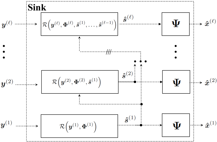
After receiving the measurements for all data types , the sink then proceeds to the data recovery stage, which is the focus of our paper, and is shown schematically in Fig. 3. Our method operates in stages, with the sink reconstructing the vectors sequentially, i.e., first , then , until . When reconstructing , the sink uses the measurements that were relayed, , the matrix , as well as the previously reconstructed vectors , which play the role of multiple side information.
Standard CS recovery algorithms [19, 22, 21], as proposed by [18, 27, 26], would require recovering each sparse vector independently from the other vectors, based only on the measurement vector . This fails to leverage inter-source correlations. We will refer to this approach as the baseline solution. Alternatively, one can apply DCS [24] to recover the ensemble of sparse vectors using the ensemble of measurements vectors and the matrices . However, as shown in our experimental results, DCS does not efficiently capture the underlying dependencies among heterogeneous data, such as various air pollutants, which have different statistical properties.
The method we propose, in contrast, leverages diverse correlated signals through copula functions [34, 35]. Copula functions, explained in detail in Section IV-A, are elements of a statistical framework to effectively capture dependencies between random variables. As will be explained in Section V, we use copula functions to integrate knowledge from other data types in the reconstruction of a given data type or, in other words, as a way to integrate multiple side information. Our experiments in Section VI show that it is exactly because it uses multiple side information signals at the recovery stage that our scheme outperforms the state-of-the-art methods in [24, 27, 29, 30, 31].
IV Statistical Modelling Using Copulas
We now describe how to model statistically heterogeneous data using copula functions. Let denote the random variable associated with the reading of source , and let be one of its realizations. In general, the data sources we consider are not independent, meaning their joint probability density function (pdf) does not factor into the product of its marginals. We will represent this joint pdf as , where is a random vector and its realization.22 2 Notice the difference in notation with respect to , which collects the samples observed from data type . We assume that each sensor observes , an independent realization of . In other words, is an i.i.d. copy of . This implies
| (6) |
We will see next how a copula function enables working with the marginals of the joint pdfs in (6), even though, as we saw before, these pdfs do not factor into the product of their marginals.
IV-A Introduction to Copulas
Suppose the random vector is supported on a continuous set and has joint cumulative distribution function (cdf)
We will denote the marginal cdfs by . The probability integral transform [48] states that, independently of the distribution of , the random variable always has uniform distribution over .
The copula function of the random vector is defined on the unit hypercube as the joint cdf of , that is,
| (7) |
where . Namely, a copula is a multivariate cdf whose marginals have uniform distribution. The following result was seminal in the development of the theory of copula functions.
Theorem IV.1 (Sklar’s theorem [34])
For any -dimensional joint cdf whose marginals are continuous, there exists a unique -dimensional copula function such that
| (8) |
The implications of Theorem IV.1 are best seen after taking the -th cross partial derivative of (8):
| (9) |
where denotes the copula density, and is the pdf of . Expression (9) tells us that the joint pdf of dependent random variables can be written as the product of the marginal pdfs, as if the variables were independent, times the copula density, which acts as a correction term. In other words, the copula density alone captures all the dependencies of the random variables. This means that finding a good model for the joint pdf boils down to finding not only accurate models for the marginal pdfs, but also an appropriate copula function to effectively capture the dependencies in the data.
IV-B Copula Families
There exist several bivariate and multivariate copula families [49, 50, 35], typically categorized into implicit and explicit. Implicit copulas have densities with no simple closed-form expression, but are derived from well known distributions. An example is the Elliptical copulas, which are associated to elliptical distributions (for example, the multivariate normal distribution), and have the advantage of providing symmetric densities. This makes them appropriate for high-dimensional distributions. Table I shows the expressions for the two mostly used Elliptical copulas: the Gaussian, and the Student’s -copula [34]. The expression for the Gaussian copula uses a standard multivariate normal distribution parameterized by the correlation matrix . In turn, the expression for the Student’s -copula uses a standard multivariate -distribution, parameterized by the correlation matrix and by the degrees of freedom . The diagonal entries of the correlation matrices are , and the non-diagonal are equal to the estimated Spearman’s values.
| Name | Parameters | Functions | |
|---|---|---|---|
| Gaussian | : correlation matrix | standard multivariate normal distribution | |
| standard univariate normal distribution | |||
| Student | correlation matrix | standard multivariate -distribution | |
| degrees of freedom | univariate -distribution |
Explicit copulas have densities with simple closed-form expressions but, being typically parameterized by few parameters, lack some modeling flexibility. The most popular explicit copulas are the Archimedean, which are parameterized by a single parameter . Specifically, an Archimedean copula is defined as [35]:
| (10) |
where is a continuous, strictly decreasing, convex function such that . The function is called generator and its pseudo-inverse, defined by
| (11) |
has to be strictly-monotonic of order [51]. Table II shows the distributions of the most popular Archimedean copulas: the Clayton, the Frank, and the Gumbel copulas [52].
For both families, the estimation of the copula parameters, e.g., the correlation matrix, is performed using training data. This will be described in detail in Section VI.
| Name | Parameter Range | Generator | |
|---|---|---|---|
| Clayton | |||
| Frank | |||
| Gumbel |
IV-C Marginal Statistics
As shown in (9), a consequence of Sklar’s theorem (Theorem IV.1) is that copula functions enable us to work with the marginal pdfs of a random vector even when its components are not independent. We will consider the following pdfs when we model the distribution of each component.
- 1.
Laplace distribution
(12) where is the scaling parameter and is the mean value for the -th data type, with .
- 2.
Cauchy (or Lorentz) distribution
(13) where is a scale parameter specifying the half-width at half-maximum, and is the location parameter.
- 3.
Non-parametric distribution via kernel density estimation (KDE) [53]
(14) where is the number of samples from data type . We use the Gaussian kernel because of its simplicity and good fitting accuracy. We also select different smoothing parameters for different data types, .
V Copula-based Belief Propagation
We now describe our reconstruction algorithm, executed at the sink node. As mentioned, the sparse vectors are reconstructed sequentially: first, , then , and so on. The reconstruction of each thus uses not only the respective measurements , but also the previously reconstructed data types as side information.
We adopt the framework of Bayesian CS [21, 54], as it naturally handles our joint statistical characterization of the correlated modalities. We start by computing the posterior distribution of the random vector , representing the sparse vectors of coefficients of data type , given the respective measurements and the first data types:
| (15) | ||||
| (16) | ||||
| (17) | ||||
| (18) |
where we excluded the arguments of the pdfs for notational simplicity. From (15) to (16), we just applied Bayes’s theorem and omitted constant terms. From (16) to (17), we used the assumption that measurements from data type given realizations of all the previous data types depend only on the value of ; in other words, the process is Markovian. Finally, from (17) to (18), we used the assumption that measurement noise at different sensors is independent, and also that each sensor observes independent realizations of the random vector (cf. Section IV). Obtaining an estimate of by minimizing the mean-squared-error or via maximum a posteriori (MAP) is challenging due to the complexity of the posterior distribution in (18). Therefore, as in [21], we use the belief propagation algorithm [36].
Our approach modifies the algorithm in [21] to take into account the previously reconstructed signals in the reconstruction of . Fig. 4 represents the factor graph associated with (18). A factor graph represents the factorization of an expression by using two types of nodes: variable nodes and factor nodes. Variable nodes are associated to the variables of the expression, in this case, the components of the vector , …, and, in Fig. 4, are represented with circles. The factor nodes are associated to the intermediate factors in the expression, in this case, the terms in (18) and, in Fig. 4, are represented with squares. Specifically, the leftmost squares in the figure represent the terms in the product , and the rightmost squares represent terms in the product .
Notice that when there is no measurement noise in the acquisition of the measurements , each factor becomes
| (19) |
where is the Dirac delta function. When the measurement noise is, for example, AWGN, then in (19) is replaced by the density of the normal distribution. Therefore, in Fig. 4, the edges from the variable nodes to the leftmost factor nodes represent the connections defined by measurement equation (cf. Section III): there is an edge between factor and variable whenever . Recall also that the nonzero entries of are .
Regarding the connections with the rightmost factor nodes in Fig. 4, notice that (9) implies that each term can be expressed as the marginal pdf times a correction term that captures information from the previously reconstructed data types. Indeed, assuming we have access to estimates of , for , there holds
| (20) | ||||
| (21) | ||||
| (22) |
where for . From (20) to (21) we used the definition of conditional density, and from (21) to (22) we simply used (9). Expression (22) depends only on and thus explains the edges from the variables nodes to the rightmost factor nodes in Fig. 4.
Belief propagation is an iterative algorithm in which each variable node sends a message to its neighbors (which are only factor nodes), and each factor node sends a message to its neighbors (which are only variable nodes). Here, represents either , for , or , for . In our case, a belief propagation message is a vector that discretizes a continuous probability distribution. For example, suppose the domain of the pdfs is , but we expect the values of the variables to be concentrated around . We can partition into bins around , e.g., . The message, in this case, would be a -dimensional vector whose entries are the probabilities that a random variable belongs to the respective bin. For instance, all the messages to and from variable node are vectors of probabilities, , which are iteratively updated and represent our belief for the (discretized) pdf of . Note, in particular, that all vectors have the same length and that all the messages to and from a variable node depend on that variable only. We represent a message from variable to factor at iteration as , and a message from factor to variable as . The messages are updated as follows:33 3 See, e.g., [21] for a more detailed account on belief propagation algorithms, including a derivation of these formulas. Note also that, for simplicity, we omit normalizing constants.
| (23) | ||||
| (24) |
where denotes the sum over all variables but , and a “product” between messages is the pointwise product between the respective vectors.
We run the message passing algorithm (23)-(24) for iterations. To obtain the final estimate of each , we first compute the vector
and select as the mid-value of the bin corresponding to the largest entry of . This gives us each component of the estimated vector of coefficients . In turn, the estimated readings are computed as .
VI Experiments
We evaluate the data recovery performance of the proposed copula-based design using synthetic data (cf. Section VI-A) as well as actual sensor readings taken from the air pollution database of the US Environmental Protection Agency (EPA) [37] (cf. Section VI-B). Furthermore, in Section VI-C, we study the impact of the proposed method on the energy consumption of the wireless devices.
VI-A Results on Synthetic Data
In order to evaluate the proposed copula-based method, we simulate the approach described in Section III. We consider the vectorized readings of two statistically dependent data types collected at a given time instance by a WSN and their compressible representations in a basis . Following existing stochastic models [55] for the generation of spatially-correlated WSN data, we assume that both and are Gaussian. We also assume that is stationary (its variance is constant across readings), while is piece-wise stationary (its variance varies across groups of readings). Taking as the DCT basis, it can be fairly assumed that the coefficients in are Gaussian, whereas the coefficients in follow the Laplace distribution44 4 As shown in [56], the Laplace distribution emerges under the assumption that the variance across the group of readings is exponentially distributed. [56]. To simulate this scenario, we generate , as follows: We draw two coupled i.i.d. uniform random vectors , with , from the bivariate Clayton or Frank copula [52]. The length of each uniform random vector is and the copulas are parameterized by and , respectively. We consider different values for and , corresponding to weak, moderate, and strong dependency, respectively. We then generate the entries of by applying the inverse cdf of with to the entries of ; similarly, the entries of are generated by applying the inverse cdf of with to the entries of . We obtain measurements —the column weight of is set to —and we assess the reconstruction of . We vary the number of measurements from to and, for each , we perform independent trials—each with a different and —and we report the average relative error as a function of .
We compare the recovery performance of two methods: the baseline method—which recovers from via Bayesian CS with belief propagation [21]—and the proposed copula-based method that recovers using and . In both methods, the length of each message vector carrying the pdf samples in the belief propagation algorithm is set to and the number of iterations to 50. In order to have a fair comparison with CS, we account for a copula mismatch in our method. Namely, we use the bivariate Gaussian copula to model the dependency between the data, where the correlation matrix is fitted on the generated data using maximum likelihood estimation [57], even though the true relation between data types is generated with the Clayton or Frank copula.
The experimental results, depicted in Fig. 5, show that—despite the copula mismatch—the proposed algorithm manages to leverage the dependency among the diverse data and thus, to systematically improve the reconstruction performance compared to the classical method [21]. The performance improvements are increasing with the amount of dependency between the signals, reaching average relative error reductions of up to 72.90% and 64.09%, for the Clayton () and the Frank copula (), respectively.
VI-B Results on Real Air Pollution Data
The AQS (Air Quality System) database of EPA [37] aggregates air quality measurements taken by more than monitoring stations, which collect hourly or daily measurements of the concentrations of six pollutants: ozone , particulate matter (PM10 and PM2.5), carbon monoxide (CO), nitrogen dioxide , sulfur dioxide , and lead (Pb). We consider a network architecture comprising a sink and nodes, where each node is equipped with sensors to measure the concentration of CO, NO2 and SO2 in the air. Using the node coordinates in the EPA database, we simulate such networks55 5 Each network is formed by nodes within only one of the following states: CA, NV, AZ, NC, SC, VA, WV, KY, TN, MA, RI, CT, NY, NJ, MD. by assuming that the transmission adheres to LoRa [58], according to which the node distance does not exceed km in urban areas and km in rural areas. From the database, we take values for each of the three pollutants—i.e., CO, NO2 and SO2—collected during the year 2015. The data are equally divided into a training and an evaluation set, without overlap.
| DCT | Haar | Daubechies-2 | Daubechies-4 | ||
|---|---|---|---|---|---|
| 0.1 | 28.8 | 19.1 | 25.50 | 23.80 | |
| 48.50 | 35.80 | 46.30 | 44.00 | ||
| 74.10 | 67.00 | 77.50 | 77.30 | ||
| CO | 0.1 | 25.90 | 16.40 | 22.60 | 19.40 |
| 44.50 | 31.20 | 40.30 | 38.70 | ||
| 70.30 | 58.20 | 69.80 | 69.20 |
VI-B1 Sparsifying Basis Selection
We first identified a good sparsifying basis for the data. Following the network architecture described in the previous paragraph, we organized the training data into blocks of readings per pollutant. In order to form a block , readings must have the same timestamp and be measured by neighboring stations, adhering to the LoRa [58] transmission distance criteria. We projected the data in each block onto different set of bases, including the discrete cosine transform (DCT), the Haar, the Daubechies-2, and the Daubechies-4 continuous wavelet transform (CWT) bases; for the CWT we experimentally found that the scale parameter led to the best compaction performance. Since the resulting representation is a compressible signal, we calculated the number of coefficients in whose the absolute value is below a given threshold . Table III reports the results for and CO, averaged over all the blocks in the training set. It shows that the DCT yielded the sparsest representations.


VI-B2 Marginal Statistics and Copula Parameters
To select the most appropriate marginal distribution for DCT coefficients of each , with , we performed fitting tests using the training set. The Laplace, the Cauchy, and the non-parametric distribution—via KDE with a Gaussian Kernel—were fitted to the data using the Kolmogorov-Smirnov test [59], with significance level set to . The results, which were averaged over all the blocks in the training set, are reported in Table IV and Fig. 6. We can observe that the Cauchy distribution gives the best fit for the CO and SO2 data, whereas the Laplace distribution best describes the statistics of the NO2 data. The parameters of the distributions were estimated via maximum likelihood estimation (MLE), resulting in , for the Cauchy distributions, and for the Laplace distribution; recall the expressions for the pdf of these distributions in (12) and (13). We also estimated the mean values of the DCT coefficients, which were very close to zero for all distributions.
We now elaborate on the estimation of the parameters of the different copulas, described in Section IV-B. Using standard MLE [57], we calculate the correlation matrix for the Gaussian copula, the pairwise correlation values of which are presented in Table V. Moreover, we estimate the correlation matrix and the degrees-of-freedom parameter for the Student’s -copula via approximate MLE [57]. The latter method fits a Student’s -copula by maximizing an objective function that approximates the profile log-likelihood for the degrees-of-freedom parameter. For the ensemble of the three pollutants we find the optimal value to be , whereas the values corresponding to each pair of pollutants are in Table V. Table V also reports the pair-wise maximum-likelihood estimates [60] of the parameter for different bivariate Archimedean copulas [cf. (10)]. We consider bivariate Archimedean copulas for their simplicity, i.e., they are parameterized by a single parameter. This, however, limits their modeling capacity and makes them less accurate than, for example, Elliptical copulas [35].
| Laplace | Cauchy | KDE | |
|---|---|---|---|
| CO | |||
| NO2 | |||
| SO2 |
| Parameters | |||
|---|---|---|---|
| Correlation | |||
| Degrees of Freedom, | |||
| (Clayton) | |||
| (Frank) | |||
| (Gumbel) |
VI-B3 Performance Evaluation of the Proposed Algorithm
We now describe how we evaluated the performance of our method against state-of-the-art reconstruction algorithms. Simulating the data collection approach described in Section III, for every vector of readings in the test dataset, we obtained its measurements as . Similar to Section VI-A, we varied the number of measurements from to and, for each , we generated different matrices (independently). We will report the average [over the ’s and over all the points in the test dataset] relative error as a function of .
In the first set of experiments, we used the NO2 data to aid the reconstruction of the CO readings and considered the following methods: (i) the proposed copula-based belief propagation algorithm, running for iterations and using five different bivariate copulas for modelling the joint distribution, namely, the Gaussian, the Student’s , the Clayton, the Frank, and the Gumbel copulas; (ii) the - minimization method;66 6 The - minimization problem (3) is solved using the code in [61]; a detailed explanation of the solver can be found therein. The experiments in [29, 31] show that such a solver finds medium-accuracy solutions to (3) efficiently. (iii) the baseline method [18, 27], which applies Bayesian CS [21] to recover the CO data independently; and, as a sanity check, (iv) simply keeping the largest (in absolute value) DCT coefficients.
Fig. 7 depicts the relative reconstruction error versus the number of measurements . It is clear that the proposed algorithm and - minimization efficiently exploited the side information and were able to improve the performance with respect to the baseline method [18, 27]. When the number of measurements was small (), the baseline method outperformed - minimization; this is because, with few measurements, the side information was actually hindering reconstruction; recall that - minimization assumes the side information to be of the same kind as the signal to reconstruct. Furthermore, it is clear that the proposed algorithm systematically outperformed - minimization [29] for all the considered copula functions. The best performance was achieved by the Student -copula function, providing average relative error reductions of up to compared to - minimization. We mention that, contrary to most results in compressed sensing, the results of Fig. 7 fail to exhibit a precise phase transition. This is because the representation of the data is not exactly sparse, only compressible. That can be seen in the plot, as the baseline method [18, 27] had a very similar performance to the DCT reconstruction, i.e., keeping only the largest DCT coefficients. This also shows that, in this case, what allowed both our method and - minimization to achieve better performance was the proper use of the (correlated) side information.
In another experiment, we reconstructed CO readings using as side information data from the other two pollutants, i.e., NO2 and SO2. Fig. 7 shows the average relative error of the proposed algorithm with one and two side information signals, and also the baseline method [18, 27]. It is clear that the more side information signals there are, the better the performance of our algorithm. We also observe that the Student’s -copula lead to a performance better than the Gaussian copula; this was because the former depends on more parameters than the latter, giving it a larger modeling capacity [62].
VI-B4 Evaluation of the Aggregated System Performance
We now describe the experiments conducted to evaluate the sequential reconstruction algorithm in which the readings are reconstructed consecutively. First, we focus on the scenario where two pollutants are measured, and we compare the following schemes: (i) the proposed sequential scheme, using the Gaussian and the Student -copula models (as shown in Section VI-B3), they perform better than other copulas); (ii) sequential data recovery using - minimization [29]; (iii) the DCS setup77 7 In the classical DCS scenario, each signal of interest is constructed by many readings of the same sensor. In order to have a fair comparison with our design, we have modified this framework by assuming that each signal of interest contains readings from different sensors observing the same source. In our experiments we used . [24]; and (iv) the baseline system in which each source is independently reconstructed using Bayesian CS[21].
The performance metric is expressed as the aggregated average relative error for all signals, , versus the total number of measurements . Fig. 8 shows that the systems based on - minimization and on DCS leverage both the inter- and intra-source dependencies between the pollutants, resulting in an improved performance with respect to the baseline system. However, when the number of measurements is small (), we see that - minimization performs poorly compared to the other methods. The proposed system with the Student -copula model systematically outperforms all the other schemes, bringing aggregated average relative error improvements of up to and against - minimization and DCS, respectively.
When three pollutants are measured, we compared all the previous schemes, except the one based on - minimization, since it does not handle multiple side information signals. Fig. 8 shows that DCS delivers superior performance compared to the baseline system, which is more noticeable when . Furthermore, the proposed design with the Student -copula model provides significant aggregated average relative error reductions of up to when compared to DCS [24]. It is important to notice that the proposed design significantly outperforms the other schemes when the number of measurements is small.
| Medium Data Recovery Quality | High Data Recovery Quality | |||||
|---|---|---|---|---|---|---|
| Baseline | - | Proposed | Baseline | - | Proposed | |
| Aggregated average relative error | 1.4046 | 1.4230 | 1.3957 | 1.1148 | 1.1044 | 1.0969 |
| Total number of measurements | 950 | 850 | 550 | 1400 | 1300 | 1050 |
VI-B5 Evaluation of the System Performance under Noise
We evaluate the robustness of the proposed successive data recovery architecture against imperfections in the communication medium. As explained in Section III, we model such imperfections using a zero-mean white Gaussian noise component additive to the measurements, where is the noise standard deviation88 8 We assume that the standard deviation of the noise is the same for all sources; hence, we drop the superscript . and is the identity matrix. In this experiment, we vary the noise level as and calculate the aggregated average relative error as a function of the total number of measurements. We first consider the case in which two pollutants are gathered by each device. The considered schemes are (i) the proposed system with successive data recovery using the copula-based algorithm (the Student’s copula is used); (ii) DCS [24], and; (iii) the baseline system [18, 27]. Figs. 9 and 9 show that the proposed system delivers superior performance compared to the competing systems for moderate () and high () noise. Moreover, we observe that the proposed algorithm is robust against noise, especially, when the number of measurements is small. In particular, the aggregated average relative error increases on average () and () with respect to the noiseless case.
In case three pollutants are measured, the proposed system systematically outperforms the DCS scheme and the baseline system, under both moderate and high noise. Moreover, the proposed design continues to demonstrate robustness against noise, with the aggregated average relative error increasing on average only () and () compared to the noiseless case. It is clear that the robustness of the proposed system increases with the number of pollutants.
VI-C Energy Consumption Analysis
We now study the impact of the proposed system on reducing the number of measurements and in turn the energy consumption of the wireless nodes, for a given data reconstruction quality. The energy consumption at each node is broken down into a sensing, processing and transmission part: [63]. The sensing part, , depends on the amount of censored data; hence, its energy consumption is the same for the proposed and the baseline system. We thus focus our comparison on the energy consumption due to the processing and transmission parts. Following a typical IoT design, we assume that the nodes are equipped with the MSP430 micro-controller [64] and that communication adheres to LoRa [58]. MSP430 architectures [64] are typically built around a 16-bit CPU running at 25 MHz, with a voltage supply of Volt and a current of A/MIPS in the active mode. As discussed in Section III, every node generates a pseudorandom number, computes the product between this number and the censored value, adds it to the sum of the previous relayed values, and sends the final value to the next node. This operation is repeated per measurement and source . Neglecting the pseudorandom number generation part, the encoding operation boils down to a multiply-and-accumulate (MAC) operation. The MSP430 CPU cycles needed for a single signed 16-bit MAC operation are 17 for a hardware implementation or between and for a software implementation [64]. Therefore, the time to perform a single MAC operation99 9 We consider the higher value on the number of cycles for software. is or . The total time to encode the measurements at each device can then be calculated as and the total processing energy as , where (•) stands for HW or SW. In order to calculate the energy consumption for transmission, we used the LoRa energy consumption calculator from Semtech [65, 66]. For a typical 12-byte payload packet with a 14 dBm power level, a current at 44 mA and a spreading factor of 7, the transmission energy consumption was estimated at 5.4 mJ. In the scenario where two pollutants (CO and NO2) are encoded [and no noise is assumed in the communication medium], Table VI reports the number of measurements and the energy consumption at the nodes for the baseline system, the system using - minimization [29], and the proposed system. It is worth observing that the processing energy is negligible compared to the energy consumed by the transceiver. It is evident that for a comparable aggregated average relative error the proposed system leads to a significant reduction in the number of transmitted measurements compared to the competition, which translates to critical energy savings at the nodes.
VII Conclusion and Future Work
We addressed the problem of data recovery from compressive measurements in large-scale WSN applications, such as air-pollution monitoring. In order to efficiently capture statistical dependencies among heterogeneous sensor data, we used copula functions [34, 35]. This enabled us to devise a novel CS-based reconstruction algorithm, built upon belief propagation [36, 67], which leverages multiple heterogeneous signals (e.g., air pollutants) as side information in order to improve reconstruction. Experiments using synthetic data and real sensor data from the USA EPA showed that the proposed scheme significantly improves the quality of data reconstruction with respect to prior state-of-the-art methods [23, 68, 29], even under sensing and communication noise. Furthermore, we showed that, for a given data reconstruction quality, the proposed scheme offers low encoding complexity and reduced radio transmissions compared to the state of the art, thereby leading to energy savings at the wireless devices. We conclude that our design effectively meets the demands of a large-scale monitoring application. Future work should concentrate on assessing the method on alternative datasets, such as the Intel-Berkeley Lab dataset [69], the dataset from the Center for Climatic Research [70], and the indoor dataset from the University of Padova [71].
References
- [1] E. Zimos, J. F. C. Mota, M. R. D. Rodrigues, and N. Deligiannis, “Bayesian compressed sensing with heterogeneous side information,” in IEEE Data Compression Conference, 2016.
- [2] E. Zimos, J. F. Mota, M. R. Rodrigues, and N. Deligiannis, “Internet-of-things data aggregation using compressed sensing with side information,” in Int. Conf. Telecomm. (ICT). IEEE, 2016.
- [3] I. F. Akyildiz and M. C. Vuran, Wireless sensor networks. John Wiley & Sons, 2010, vol. 4.
- [4] C. Liu, K. Wu, and J. Pei, “An energy-efficient data collection framework for wireless sensor networks by exploiting spatiotemporal correlation,” IEEE Trans. Parallel Distrib. Syst., vol. 18, no. 7, pp. 1010–1023, 2007.
- [5] S. Yoon and C. Shahabi, “The clustered aggregation (CAG) technique leveraging spatial and temporal correlations in wireless sensor networks,” ACM Trans. Sensor Net., vol. 3, no. 1, p. 3, 2007.
- [6] H. Gupta, V. Navda, S. Das, and V. Chowdhary, “Efficient gathering of correlated data in sensor networks,” ACM Trans. Sensor Net., vol. 4, no. 1, p. 4, 2008.
- [7] M. Vecchio, R. Giaffreda, and F. Marcelloni, “Adaptive lossless entropy compressors for tiny IoT devices,” IEEE Trans. Wireless Commun., vol. 13, no. 2, pp. 1088–1100, 2014.
- [8] D. I. Sacaleanu, R. Stoian, D. M. Ofrim, and N. Deligiannis, “Compression scheme for increasing the lifetime of wireless intelligent sensor networks,” in European Signal Process. Conf. (EUSIPCO), 2012, pp. 709–713.
- [9] M. Crovella and E. Kolaczyk, “Graph wavelets for spatial traffic analysis,” in Annu. Joint Conf. IEEE Comput. and Commun. (INFOCOM), vol. 3, 2003, pp. 1848–1857.
- [10] A. Ciancio, S. Pattem, A. Ortega, and B. Krishnamachari, “Energy-efficient data representation and routing for wireless sensor networks based on a distributed wavelet compression algorithm,” in Int. Conf. Inform. Process. Sensor Networks. ACM, 2006, pp. 309–316.
- [11] J. Acimovic, B. Beferull-Lozano, and R. Cristescu, “Adaptive distributed algorithms for power-efficient data gathering in sensor networks,” in International Conference on Wireless Networks, Communications and Mobile Computing, vol. 2. IEEE, 2005, pp. 946–951.
- [12] Z. Xiong, A. D. Liveris, and S. Cheng, “Distributed source coding for sensor networks,” IEEE Signal Process. Mag., vol. 21, no. 5, pp. 80–94, 2004.
- [13] V. Stankovic, A. D. Liveris, Z. Xiong, and C. N. Georghiades, “On code design for the slepian-wolf problem and lossless multiterminal networks,” IEEE Trans. Inf. Theory, vol. 52, no. 4, pp. 1495–1507, 2006.
- [14] N. Deligiannis, E. Zimos, D. Ofrim, Y. Andreopoulos, and A. Munteanu, “Distributed joint source-channel coding with copula-function-based correlation modeling for wireless sensors measuring temperature,” IEEE Sensor J., vol. 15, no. 8, pp. 4496–4507, 2015.
- [15] F. Chen, M. Rutkowski, C. Fenner, R. C. Huck, S. Wang, and S. Cheng, “Compression of distributed correlated temperature data in sensor networks,” in IEEE Data Compression Conf. (DCC), 2013, pp. 479–479.
- [16] D. L. Donoho, “Compressed sensing,” IEEE Trans. Inf. Theory, vol. 52, pp. 1289–1306, 2006.
- [17] E. J. Candès and M. B. Wakin, “An introduction to compressive sampling,” IEEE Signal Process. Mag., vol. 25, no. 2, pp. 21–30, 2008.
- [18] J. Haupt, W. U. Bajwa, M. Rabbat, and R. Nowak, “Compressed sensing for networked data,” IEEE Signal Process. Mag., vol. 25, no. 2, pp. 92–101, 2008.
- [19] J. Tropp and A. C. Gilbert, “Signal recovery from random measurements via orthogonal matching pursuit,” IEEE Trans. Inf. Theory, vol. 53, no. 12, pp. 4655–4666, 2007.
- [20] T. Blumensath and M. E. Davies, “Iterative hard thresholding for compressed sensing,” Applied Computational Harmonic Analysis, vol. 27, no. 3, pp. 265–274, 2009.
- [21] D. Baron, S. Sarvotham, and R. G. Baraniuk, “Bayesian compressive sensing via belief propagation,” IEEE Trans. Signal Process., vol. 58, no. 1, pp. 269–280, 2010.
- [22] D. L. Donoho, A. Maleki, and A. Montanari, “Message-passing algorithms for compressed sensing,” Proc. Nat. Academy Sci., vol. 106, no. 45, pp. 18 914–18 919, 2009.
- [23] J. Haupt and R. Nowak, “Signal reconstruction from noisy random projections,” IEEE Trans. Inf. Theory, vol. 52, no. 9, pp. 4036–4048, 2006.
- [24] M. F. Duarte, S. Sarvotham, D. Baron, M. B. Wakin, and R. G. Baraniuk, “Distributed compressed sensing of jointly sparse signals,” in Asilomar Conf. Signals, Syst., Comput., 2005, pp. 1537–1541.
- [25] R. Masiero, G. Quer, D. Munaretto, M. Rossi, J. Widmer, and M. Zorzi, “Data acquisition through joint compressive sensing and principal component analysis,” in IEEE Global Telecommun. Conf. (GLOBECOM). IEEE, 2009, pp. 1–6.
- [26] G. Quer, R. Masiero, G. Pillonetto, M. Rossi, and M. Zorzi, “Sensing, compression, and recovery for wsns: Sparse signal modeling and monitoring framework,” IEEE Trans. Wireless Commun., vol. 11, no. 10, pp. 3447–3461, 2012.
- [27] C. Luo, F. Wu, J. Sun, and C. W. Chen, “Efficient measurement generation and pervasive sparsity for compressive data gathering,” IEEE Trans. Wireless Commun., vol. 9, no. 12, pp. 3728–3738, 2010.
- [28] S. Lee, S. Pattem, M. Sathiamoorthy, B. Krishnamachari, and A. Ortega, “Spatially-localized compressed sensing and routing in multi-hop sensor networks,” in International Conference on GeoSensor Networks. Springer, 2009, pp. 11–20.
- [29] J. F. C. Mota, N. Deligiannis, and M. R. D. Rodrigues, “Compressed sensing with prior information: Strategies, geometry, and bounds,” IEEE Trans. Inf. Theory, vol. 63, no. 7, pp. 4472–4496, 2017.
- [30] J. F. C. Mota, L. Weizman, N. Deligiannis, Y. Eldar, and M. R. Rodrigues, “Reference-based compressed sensing: A sample complexity approach,” in IEEE Int. Conf. Acoust., Speech Signal Process. (ICASSP), 2016.
- [31] J. F. Mota, N. Deligiannis, and M. R. Rodrigues, “Compressed sensing with side information: Geometrical interpretation and performance bounds,” in IEEE Global Conf. Signal and Inform. Process. (GlobalSIP), 2014, pp. 512–516.
- [32] F. Renna, L. Wang, X. Yuan, J. Yang, G. Reeves, R. Calderbank, L. Carin, and M. R. Rodrigues, “Classification and reconstruction of high-dimensional signals from low-dimensional features in the presence of side information,” IEEE Trans. Inf. Theory, vol. 62, no. 11, pp. 6459–6492, 2016.
- [33] Y. Liu, X. Zhu, and L. Zhang, “Noise-resilient distributed compressed video sensing using side-information-based belief propagation,” in IEEE Int. Conf. Network Infrastructure Digit. Content (IC-NIDC), 2012, pp. 350–390.
- [34] M. Sklar, Fonctions de répartition à n dimensions et leurs marges. Un. Paris 8, 1959.
- [35] R. B. Nelsen, An Introduction to Copulas. Secaucus, NJ, USA: Springer-Verlag New York, Inc., 2006.
- [36] D. J. MacKay, Information theory, inference and learning algorithms. Cambridge University Press, 2003.
- [37] [Online]. Available: http://www3.epa.gov/airdata/.
- [38] D. L. Donoho and X. Huo, “Uncertainty principles and ideal atomic decomposition,” IEEE Trans. Inf. Theory, vol. 47, no. 7, pp. 2845–2862, 2001.
- [39] E. J. Candes and T. Tao, “Decoding by linear programming,” IEEE Trans. Inf. Theory, vol. 51, no. 12, pp. 4203–4215, 2005.
- [40] V. Chandrasekaran, B. Recht, P. A. Parrilo, and A. S. Willsky, “The convex geometry of linear inverse problems,” Found. Computational Mathematics, vol. 12, no. 6, pp. 805–849, 2012.
- [41] J. F. C. Mota, N. Deligiannis, A. C. Sankaranarayanan, V. Cevher, and M. R. Rodrigues, “Dynamic sparse state estimation using minimization: Adaptive-rate measurement bounds, algorithms and applications,” in IEEE Int. Conf. Acoust., Speech Signal Process. (ICASSP), 2015.
- [42] N. Vaswani and W. Lu, “Modified-CS: Modifying compressive sensing for problems with partially known support,” IEEE Trans. Signal Process., vol. 58, no. 9, 2010.
- [43] J. Scarlett, J. S. Evans, and S. Dey, “Compressed sensing with prior information: Information-theoretic limits and practical decoders,” IEEE Trans. Signal Process., vol. 61, no. 2, pp. 427–439, 2013.
- [44] M. A. Khajehnejad, W. Xu, A. S. Avestimehr, and B. Hassibi, “Weighted minimization for sparse recovery with prior information,” in IEEE Int. Symp. Inf. Theory (ISIT), 2009, pp. 483–487.
- [45] S. Oymak, M. A. Khajehnejad, and B. Hassibi, “Recovery threshold for optimal weight minimization,” in IEEE Int. Symp. Inf. Theory (ISIT), 2012, pp. 2032–2036.
- [46] M. Trocan, T. Maugey, J. E. Fowler, and B. Pesquet-Popescu, “Disparity-compensated compressed-sensing reconstruction for multiview images,” in IEEE Int. Conf. Multimedia and Expo (ICME), 2010, pp. 1225–1229.
- [47] R. G. Gallager, “Low-density parity-check codes,” IRE Trans. on Inform. Theory, vol. 8, no. 1, pp. 21–28, 1962.
- [48] C. Genest and L.-P. Rivest, “On the multivariate probability integral transformation,” Stat. & Probability Lett., vol. 53, no. 4, pp. 391–399, 2001.
- [49] H. Joe, Multivariate models and multivariate dependence concepts. CRC Press, 1997, vol. 73.
- [50] C. Genest and J. Mackay, “The joy of copulas: bivariate distributions with uniform marginals,” Amer. Statistician, vol. 40, no. 4, pp. 280–283, 1986.
- [51] A. J. McNeil and J. Nešlehová, “Multivariate archimedean copulas, d-monotone functions and ℓ₁-norm symmetric distributions,” Ann. Stat., pp. 3059–3097, 2009.
- [52] A. J. McNeil, R. Frey, and P. Embrechts, Quantitative risk management: concepts, techniques and tools. Princeton University Press, 2005.
- [53] G. G. Roussas, An introduction to probability and statistical inference. Academic Press, 2003.
- [54] S. Ji, Y. Xue, and L. Carin, “Bayesian compressive sensing,” IEEE Trans. Signal Process., vol. 56, no. 6, pp. 2346–2356, 2008.
- [55] D. Zordan, G. Quer, M. Zorzi, and M. Rossi, “Modeling and generation of space-time correlated signals for sensor network fields,” in IEEE Global Telecommunications Conference (GLOBECOM), 2011, pp. 1–6.
- [56] E. Y. Lam and J. W. Goodman, “A mathematical analysis of the DCT coefficient distributions for images,” IEEE Trans. Image Process., vol. 9, no. 10, pp. 1661–1666, 2000.
- [57] E. Bouyé, V. Durrleman, A. Nikeghbali, G. Riboulet, and T. Roncalli, “Copulas for finance-a reading guide and some applications,” Available: http://ssrn.com/abstract=1032533, 2000.
- [58] [Online]. Available: https://www.lora-alliance.org/.
- [59] F. J. Massey Jr, “The Kolmogorov-Smirnov test for goodness of fit,” Amer. Statistical Assoc. J., vol. 46, no. 253, pp. 68–78, 1951.
- [60] C. Genest and L.-P. Rivest, “Statistical inference procedures for bivariate Archimedean copulas,” Amer. Statistical Assoc. J., vol. 88, no. 423, pp. 1034–1043, 1993.
- [61] “João Mota,” https://github.com/joaofcmota/cs-with-prior-information/docs/docs.pdf.
- [62] W. Breymann, A. Dias, and P. Embrechts, “Dependence structures for multivariate high-frequency data in finance,” Quantitative Finance, vol. 3, no. 1, pp. 1–14, 2003.
- [63] O. Landsiedel, K. Wehrle, and S. Gotz, “Accurate prediction of power consumption in sensor networks,” in IEEE Workshop on Embedded Networked Sensors (EmNetS). IEEE, 2005, pp. 37–44.
- [64] T. Instruments, “The MSP430 hardware multiplier function and applications,” Application Report, pp. 1–30, 1999.
- [65] “Semtech LoRa Modem Design Guide,” www.semtech.com/images/datasheet/LoraLowEnergyDesign_STD.pdf.
- [66] “Semtech,” http://www.semtech.com/wireless-rf/rf-transceivers/sx1272.
- [67] R. G. Cowell, Probabilistic networks and expert systems: Exact computational methods for Bayesian networks. Springer Science & Business Media, 2006.
- [68] D. Baron, M. F. Duarte, S. Sarvotham, M. B. Wakin, and R. G. Baraniuk, “An information-theoretic approach to distributed compressed sensing,” in 45th Annu. Allerton Conf. Commun., Control, and Computing, 2005.
- [69] P. Bodik, W. Hong, C. Guestrin, S. Madden, M. Paskin, and R. Thibaux. (2004, Feb.) Intel lab data. [Online]. Available: http://db.csail.mit.edu/labdata/labdata.html
- [70] C. J. Willmott and K. Matsuura. (2009, Aug.) Global climate resource pages. [Online]. Available: http://climate.geog.udel.edu/∼climate/
- [71] R. Crepaldi, S. Friso, A. Harris, M. Mastrogiovanni, C. Petrioli, M. Rossi, A. Zanella, and M. Zorzi, “The design, deployment, and analysis of signetlab: a sensor network testbed and interactive management tool,” in Int. Conf. Testbeds and Research Infrastructure for the Development of Networks and Communities (TridentCom), 2007, pp. 1–10.