Calvera: A low-mass strangeon star torqued by debris disk?

The ROSAT All-Sky Survey discovered a high galactic latitude ($b=37\arcdeg$) compact object, 1RXS J141256.0+792204 [58], which was then identified as an isolated neutron star (INS, hereafter “NS” refers to all kinds of pulsar-like compact objects) candidate. The fact that this INS is discovered after the seven radio-quiet and thermally emitting X-ray dim isolated neutron star (XDINS), the Magnificent Seven [see 25, 35, for reviews], leads it to be nicknamed as “Calvera”. Calvera, in particular, is a puzzling source that has some confusion in the classification among the neutron star family.

Calvera exhibits X-ray pulsations with period $P=59\,\mathrm{ms}$ [76] and spin-down rate $\dot{P}=3.2\times 10^{-15}\,\mathrm{s\,s^{-1}}$ [27, 29], making its location in the $P-\dot{P}$ diagram (Figure 1) far from the Magnificent Seven class, which are slowly rotating $(P\sim 3-11\,\mathrm{s})$ NSs. It is also speculated that Calvera might be a candidate of the central compact object [58, 76, 23, CCO,]. However, Calvera presents a larger dipole magnetic field [60] and there is still no conclusive evidence for the host supernova remnant [76]. Alternatively, there are suggestions that the magnetic field ($\sim 10^{12}\,\mathrm{G}$) of CCO is buried by prompt fall-back of a small amount of supernova ejecta [31, 68, 7]; therefore, Calvera could be a descendant of the CCO reemerging the magnetic field [27].

It is odd that deep search failed to detect the radio emission from this source [30, 76]. The non-detection of radio emission from Calvera can not be simply attributed to the unfavored beaming effect since emission features are nor found in gamma-rays [26, 27] which commonly correspond to a larger beaming angle. This can be explained by a distant location of Calvera [61, e.g.,$1.5-5\,\mathrm{kpc}$,], but that would place it high above the Galactic disk and cause problem for its birth place, given its rather small proper motion [29, $69\pm 26\,\mathrm{mas\,yr^{-1}}$,]. Moreover, attempts also failed in searching for non-thermal emission feature in the soft X-ray band [76, 27]. All these observational facts could contain hints for an inactive-magnetosphere (i.e., dead) scenario which will be discussed in this work.

The dead-pulsar-scenario is hardly understood in the framework of NS due to its high position above the NS death line (Figure 1). Spectral fits for Calvera with neutron star atmosphere model result in small emission-radius-to-distance ratio, which forces [61] to conclude a large distance. Alternatively, we explore the possibility that Calvera is a small radius strangeon star. “Strangeon” [41], previously known as “strange quark-cluster” [73] is a prospective candidate for the pulsar constituent and have been successfully applied to solve problems including glitches [78]; high mass NS [39, 40]; ultra low-mass and small radius NS [43]. A radiative model of the strangeon star atmosphere [72, 71, SSA,] is also developed to solve the optical/ultra-violet(UV) excess problem [70, 67, 36] and the Rayleigh-Jeans deviation problem [36] of XDINSs. The luminosity of strangeon star is maintained by accretion [72] that would also exert a braking torque accounting for the spin-down rate. It is proposed here that Calvera is a low-mass strangeon star with an inactive magnetosphere and probably braked by the accretion flow. In this picture, Calvera and XDINSs, having similar radiative properties, can be understood as strangeon stars at different stages of the evolution.

We introduce the data reduction procedure and spectra modeling in Section II and III, respectively. In Section IV we constrain the parameters of Calvera as an isolated dead-pulsar while in Section V we re-consider this issue by taking into account the accretion effects. We discuss the nature of Calvera in Section VI. Summary and future possible observations in constraining the nature of Calvera are presented in Section VII.

Since the first detection by ROSAT [69], X-ray observations on Calvera have been made several times by Swift [58], XMM-Newton [76] and Chandra [60, 27, 29]. Despite numerous attempts in modeling the X-ray spectra, the nature of Calvera still remains open. In this work, we make a joint analysis [61, also see,] for the spectral data obtained by XMM-Newton and Chandra to further investigate the properties of Calvera. Swift data are omitted due to its limited counting statistics [58].

It is suggested that pulsars could be strangeon stars [41]. A strangeon star can be thought as a 3-flavored gigantic nucleus, and strangeons (coined by combining “strange nucleons”) are its constituent as an analogy of nucleons which are the constituent of a normal (micro) nucleus. The radiative model of the strangeon star atmosphere was put forth by [72]. For an isolated strangeon star, normal matter (i.e., composed by u, d quarks) accreted onto the stellar surface can not be converted to strangeons (i.e., strangeonization) instantly because the collision timescale $\tau_{\mathrm{col}}\sim 10^{-22}-10^{-20}\,\mathrm{s}$ is far smaller than that of the weak interaction $\tau_{\mathrm{weak}}\sim 10^{-7}\,\mathrm{s}$. Therefore the unconverted matter would be re-bounced and form a thermally emissive atmosphere. The flux can be described as

where $F_{\nu}$ is the flux at frequency $\nu$ and $B_{\nu}$ is the blackbody spectrum. $\tau_{\infty}(\nu)$ is the observed optical depth, with the factor $2$ accounting for the surface reflection [71], and can be expressed as

where $n_{\mathrm{i}0}$ is the ion density at bottom, $T_{\mathrm{i}}$ and $T_{\mathrm{e}}$ are the ion and electron temperatures, respectively, and $R$ is the stellar radius. We use the notation $y={n^{2}_{\mathrm{i0}}(kT_{\mathrm{i}})_{\mathrm{keV}}}/R_{\mathrm{km}}\sim 10^{42}\,\mathrm{keV\,km^{-1}\,cm^{-6}}$ for these degenerate parameters which is different from the one used in [72, 71] by $1/R$ (the SSA model with this new definition is now uploaded to Xspec for public use). At lower energies (i.e., optical/UV bands), the optical depths are high and the radiation behaves like a blackbody. Whereas for soft X-rays, the typical optical depths are small and the flux can be approximated by $F_{\nu}=2\tau(\nu)B_{\nu}$, which is lower than a pure blackbody spectrum. Therefore, extrapolating the blackbody spectrum obtained in the X-ray band will meet the optical/UV excess problem [36]. The low optical depths in X-rays have two consequences: (1) Parameter $y$ is partially degenerate with the normalization $(R_{\mathrm{km}}/d_{10\,\mathrm{kpc}})^{2}$ and the two cannot be determined simultaneously without the knowledge of the optical/UV flux. (2) Since the optical/UV excess is expected from a simple extrapolation of the blackbody spectrum in the X-rays, we can use the extrapolation of the pure blackbody fit for X-rays at optical band as a lower limit for the normalization. On the other hand, optical upper limit were obtained by Gemini-North [58, g band,] and Gran Telescopio Canarias [61, GTC, $g^{\prime},r^{\prime}$ bands,], which give the upper limit of the normalization.

The phase-averaged spectral analysis was performed simultaneously for data obtained with different detectors or at different times, allowing only the parameter $y$ to vary independently to account for possible cross-calibration uncertainties. The fit was conducted with blackbody model (BB) and SSA model with fixed $N_{\mathrm{H}}$ [34, F, with $N_{\mathrm{H}}$ fixed to the Galactic value,] or $R^{\infty}$ (M1, M2). The upper limit of the normalization (M1) was chosen such that the extrapolated spectrum meet the upper limit at GTC $g^{\prime}$ band. The lower limit (M2) was chosen such that the extrapolated spectrum converges with the blackbody fit at lower energies (e.g., $\sim\mathrm{eV}$). Results are listed in Table 2 and illustrated in Figure 2.

As is shown in [60], [76] and [27], single thermal spectra, either blackbody or pure hydrogen atmospheric model (NSA), can not provide decent fit, and two thermal components is required. The first joint fit for all available data is performed by [61], who use a single component magnetized hydrogen atmosphere model to account for the inhomogeneities of the stellar surface. Assuming a magnetic field $B=10^{12}\,\mathrm{G}$, they obtain good fits in spite of the viewing geometry. These results are broadly consistent in the sense that $T^{\infty}\sim 200\,\mathrm{eV}$ for blackbody models and $T^{\infty}\lesssim 100\,\mathrm{eV}$ for NSA models and emission area $R^{\infty}/d=2-4\,\mathrm{km\,kpc^{-1}}$[58, 60, 76, 27, 61]. In our SSA model, we obtain a higher temperature at $\gtrsim 0.6\,\mathrm{keV}$ and rather unconstrained radius $R^{\infty}/d=0.4-10\,\mathrm{km\,kpc^{-1}}$. [76] report that two-thermal models result in $N_{\mathrm{H}}$ larger than the Galactic value while we find that acceptable $N_{\mathrm{H}}$ values can be achieved assuming smaller $R^{\infty}/d$ (F and M2). The small stellar radii in the magnetized NSA model lead to the conclusion of a large distance [61, $1.5-5\,\mathrm{kpc}$,], however this is not a problem for the SSA model since strangeon star can be a few kilometers in radius.

Absorption features about $0.6-0.7\,\mathrm{keV}$ are also reported as lines [60, 76, 61] or edges [76]. We conducted similar fitting procedure and find that absorption edges or Gaussian absorption lines equally improve the fit for model F, M1 and M2. The results for the SSA model multiplied by a gabs model are list in Table 2. The additional absorption line is found at $0.73\pm 0.03\,\mathrm{keV}$, consistent with [61]. The presence of absorption line is often attributed to the magnetic field. In this case, the absorption line might indicate $B=6\times 10^{10}\,\mathrm{G}$ assuming electron cyclotron of neutron star, or $B=1.2\times 10^{11}\,\mathrm{G}$ for stangeon star hydrocyclotron [74].

In the vacuum gap model for radio emission of neutron stars, [57] propose the idea of death line, below which the electric potential of the gap region is too low ($<\Phi_{c}=10^{12}\mathrm{\,V}$) to generate electron-positron pairs for curvature radiation. The maximum potential drop ($\Phi_{\mathrm{m}}$) above the surface of a neutron star is

which yields the death line

on the premise that gap sparking could occur if $\Phi_{\mathrm{m}}>10^{12}\,\mathrm{V}$. Assuming that magnetic dipole radiation accounts for the spin-down, we plot the death lines on the $P-\dot{P}$ diagram (Figure 1) for typical neutron star radius $R=10\,\mathrm{km}$ (red dotted line) and smaller strangeon star radii (red solid lines). Note that strangeon star with smaller radius (i.e., smaller momentum inertia) would exhibit larger magnetic field than that indicated by the dashed lines in Figure 1. To meet the criterion that Calvera is dead, the upper limit for the stellar radius is $0.66\,\mathrm{km}$, which yields a stellar mass $M=3\times 10^{-4}\,M_{\odot}$. Therefore, in the context of dead pulsar, Calvera can be interpreted as a low-mass strangeon star. However, these values are extreme even for strangeon stars. This problem could be alleviated if alternative mechanisms contribute to the spin-down. In our model (see Section V), the X-ray emission is maintained by the accretion (with a rate $\dot{M}_{\mathrm{X}}=1.2\times 10^{12}d_{\mathrm{kpc}}^{2}\,\mathrm{g\,s^{-1}}$ on to the surface) which could also provide a torque braking the rapid-rotating low-mass star and accounting for the observed $\dot{P}$.

The detailed mechanism of the accretion has significant impact on the long-term evolution and leads to distinct observational consequences. Two kinds of accretion source are discussed in literature.

Interstellar medium (ISM) accretion is first proposed by [51] to understand the X-ray luminosity of INS [63, 9, also see Treves et al. 64 for reviews]. In this scenario, old INS traveling slowly through dense ISM accrete efficiently and exhibit less luminous ($\lesssim 10^{31}\,\mathrm{erg\,s^{-1}}$) thermal soft X-ray spectra. This model may explain the optical excess from the X-ray extrapolation [75] that is supported by succedent observations [36, e.g.,].

However, the relatively high proper motion and low ambient ISM density of XDINS cast doubts on the ISM accretion picture. Alternatively, it is reasonable that not all matter are expelled in the supernova explosion [14, 13] and a fractional infalling material may form a fall-back disk. The propeller or accretion torques of the disk can explain the high spin-down rate of neutron stars [1, 12, 18, 16, 6, 17] including XDINSs, the anomalous X-ray pulsars and soft gamma-ray repeaters [AXPs and SGRs, see 50, 37, for reviews], the latter are otherwise interpreted as magnetars [62]. Especially, in the picture of [1], XDINSs, AXPs and SGRs which populate similar region in the $P-\dot{P}$ diagram can be unified by the asymptotic propeller/accretion mechanism with alternative pathways. In this scenario, the X-ray luminosity of AXP/SGR is caused by accretion [6] while that of XDINS is produced by energy dissipation in the neutron star [1, 2] or by intrinsic cooling [16], i.e., accretion onto the stellar surface is not necessarily assumed in the propeller phase. However, matter inflows are observed in simulations of ISM accretion propeller [56] as well as disk accretion propeller [55] and the portion of the accreting matter may be sufficient to maintain the SSA radiation.

Nevertheless, the NS-disk system is not expected to reside in vacuum. Therefore, we propose here that ISM regulates the debris/fall-back disk accretion as a supplement and can be the dominant accretion source in the late phase when the fall-back material depletes. In this ISM-fed debris disk accretion (IFDA) picture, we expect $\dot{M}_{\mathrm{A}}>\dot{M}_{\mathrm{X}}>\dot{M}_{\mathrm{B}}$ when the fall-back system forms, where $\dot{M}_{\mathrm{B}}$ is the ISM accretion rate at the Bondi radius [10] and ${\dot{M}}_{\rm A}$ is the accretion rate at the Alfvén radius [22]. Note that $\dot{M}_{\mathrm{A}}$ decreases as the disk loses its mass gradually through accretion and propeller wind. In the late phase of the evolution, the system will reach an equilibrium at $\dot{M}_{\mathrm{X}}=\dot{M}_{\mathrm{B}}<\dot{M}_{\mathrm{A}}$ where the ISM accretion fully accounts for the NS luminosity. At this stage, a disk structure could remain but it would become thicker as it is fed by the ISM accretion and $\dot{M}_{\mathrm{A}}$ does not decrease over time. If the initial mass of the fall-back disk is small, the system could also evolve to the spherical ISM accretion regime.

We assume that the fall-back disk is formed, or maintained by the ISM, and is associated with Calvera. The accreted matter fall almost Keplerianly towards the Alfvén radius $r_{\mathrm{A}}$[22]

where $B_{12}$ is the surface magnetic field in units of $10^{12}\,\mathrm{G}$, $R_{\mathrm{km}}$ the stellar radius in units of $\mathrm{km}$, $M_{\mathrm{1}}$ the stellar mass in units of $M_{\mathrm{\odot}}$, $\dot{M}_{\mathrm{A},10}$ is the accretion rate at $r_{\mathrm{A}}$ in units of $10^{10}\,\mathrm{g\,s^{-1}}$. Matter accumulated at $r_{\mathrm{A}}$ will be forced to co-rotate with the NS and most of the mass would be expelled centrifugally due to the propeller effect [33]. Consequently, the co-rotation and deflection of the matter would exert a negative torque $N$ on the star which contributes to the spin-down of the pulsar [44],

where $\Omega_{\mathrm{K}}(r_{\mathrm{A}})=(GM/r_{\mathrm{A}}^{3})^{1/2}$ is the Keplerian angular velocity at $r_{\mathrm{A}}$. The factor $\chi$ is introduced to account for the the inefficiency of the propeller effect ($0<\chi<1$). This formula reduces to the prevailing form when $\chi=1$ [46, 12]. We assume the momentum inertia of the star to be $I=MR^{2}/2$ and the mass-radius relation for a low-mass strangeon star can be approximated by $M=4\pi\rho R^{3}/3$, where the density $\rho$ is a few times the nuclear density $\rho_{\mathrm{n}}$ [39, 38, 24]. We fix $\rho=2\rho_{\mathrm{n}}$. Combining equation (5) and (6), we obtain

where the fastness $\omega_{\mathrm{s}}=\Omega/\Omega_{\mathrm{K}}(r_{\mathrm{A}})$ and $\omega_{\mathrm{s}}>1$ in the propeller phase. Substituting $\dot{M}_{\mathrm{A}}$ into $\omega_{\mathrm{s}}$, we see the bimodality of equation (7), i.e, a “rapid” branch of solution with $\omega_{\mathrm{s}}>\omega_{\mathrm{c}}$ and the “slow” branch on the opposite, where $\omega_{\mathrm{c}}=(2/(2-\chi))^{1/\chi}$.

Most of the mass accreted to the the Alfvén radius are expelled and only a small portion of the matter are accumulated onto the strangeon star surface [55], i.e., $\dot{M}_{\mathrm{A}}=\eta\dot{M}_{\mathrm{X}}$ with $\eta>1$. $\dot{M}_{\mathrm{X}}$ can be inferred from the X-ray luminosity, $L_{\mathrm{X}}=4\pi d^{2}F_{\mathrm{X}}\approx 0.1\dot{M}_{\mathrm{X}}c^{2}$. We use the flux obtained by the spectral fit $F_{\mathrm{X},0.3-10\,\mathrm{keV}}=9.0\times 10^{-13}\,\mathrm{erg\,cm^{-2}\,s^{-1}}$ for calculation. The factor $0.1$ is the approximate energy conversion efficiency which is dominated by the gravitational potential for massive star and by the strangeonization energy release for low-mass star.

We present the parameter space of $B$ and $R$ in Figure 3 and 4. The red curve is the upper limit of the stellar radius beyond which the surface electric potential would exceed $\Phi_{\mathrm{c}}$ and the NS would be radio active (equation 4). Contours for $\eta d_{\mathrm{kpc}}^{2}$ are in solid black lines. According to the definition $\eta>1$ and the speculation that Calvera can be as close as $\sim 0.3\,\mathrm{kpc}$ [29], $\eta d_{\mathrm{kpc}}^{2}=0.1$ can be regarded as a lower limit which yields $B\lesssim 10^{11}\,\mathrm{G}$. The black dashed line is the contour for $\dot{P}_{\mathrm{dip}}$ and the shaded area on the right is prohibited. The blue dotted lines are the $\omega_{\mathrm{s}}$ contour and the shaded area on the left is also banned since there is no solution to equation 7. The ratio of matter permeate through the Alfvén radius is confusing [56, 55] and therefore left the upper limit of $\eta d_{\mathrm{kpc}}^{2}$ highly uncertain. However, the intersection point of the blue line and the red line provides the upper limit of Calvera ($R\lesssim 4\,\mathrm{km},M\lesssim 0.1\,M_{\odot}$, regardless of $\chi$), which yields a negligible redshift factor $(1-2GM/c^{2}R)^{-1/2}\lesssim 1.1$. Most of the parameter space agree with a low magnetic field $B<10^{11}\,\mathrm{G}$. The matter accreted to the polar cap diffuse across the star surface with a timescale $\tau\propto B^{2}$ [72] and can cover the whole surface for a small $B$. Therefore, we assume $R=R^{\infty}$ in the following discussion.

Jointing the parameters constrained by spectral modeling and the dead-pulsar criterion, we plot in Figure 5 the contours with respect to the stellar (radiation) radius $R^{\infty}$ and the distance $d$ in the $\chi=1$ case. The upper and lower limits of the spectral normalization are plotted as black solid lines. The colorful lines within the permitted space represent different combinations of $\eta$ and $B$ and color-coded by $B$. The contour lines are cut off at the maximum radii (dashed lines) regarding to the value of $B$. The maximum radius is defined by both the death line criterion and the fastness criterion, therefore a lower magnetic field might corresponds to a smaller maximum radius (see Figure 3 and 4). The logarithm of $\eta$ is tagged below each contour line. In the rapid branch (the upper panel), the contours of $\eta$ begin at larger radii for larger $B$, i.e., a smaller maximum radius. Therefore, beyond a certain value of $B=10^{11}\,\mathrm{G}$, no reasonable $\eta$ can satisfy the upper limit in the optical band. In the slow branch (the lower panel), the parameter space is less crowded. However, the allowed space for a high $B$ requires a large permeate fraction ($\eta>10^{6}$, the purple lines) that far exceeds the values obtained from simulations [56, 55, $\lesssim 15$,]. We conclude that $B\lesssim 10^{11}\,\mathrm{G}$.

According to the observed flux of Calvera, $\dot{M}_{\mathrm{X}}=1.2\times 10^{12}\,d^{2}_{\mathrm{kpc}}\,\mathrm{g\,s^{-1}}$. For ISM accretion, the accretion rate at the Bondi radius [10] is

where $\rho_{\infty}$ is the ISM density, assumed to be $10^{-24}\rho_{24}\,\mathrm{g\,cm^{-3}}$, $v$ the speed of the star which is inferred from the proper motion measurement to be $v_{\perp}=286\pm 110\,d_{\mathrm{kpc}}\,\mathrm{km\,s^{-1}}$ [29]. This results in $\dot{M}_{\mathrm{B}}=10^{7}\,\rho_{24}M_{1}^{2}d_{\mathrm{kpc}}^{-3}\,\mathrm{g\,s^{-1}}$ and

Even for a very small $d$ (e.g., $0.1\,\mathrm{kpc}$), the matter accretes on the stellar surface faster than the Bondi accretion and $\dot{M}_{\mathrm{A}}=\eta\dot{M}_{\mathrm{X}}\approx 10^{11-15}\,\mathrm{g\,s^{-1}}$ is even higher. The latter rate is typical for a fall-back disk of $10^{5}\,\mathrm{yr}$ [3, 18], indicating that Calvera is at the early phase of the IFDA evolution, which is often expected from a pulsar with small period.

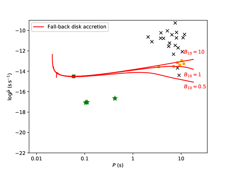
We illustrate the evolution of Calvera in Figure 6, assuming $R=2\,\mathrm{km}$ and different $B$ values. The decrease of the accretion rate of the fall-back disk is modeled by a power-law [47] $\dot{M}_{\mathrm{A}}=\dot{M}_{0}(t/T)^{-\alpha}$ (red lines). We set $T=1000\,\mathrm{s}$ and the current age of Calvera to be the characteristic age $3.2\times 10^{5}\,\mathrm{yr}$ but the detailed values are not very important. $\alpha=7/6$ is adopted from [44] which is similar to that in [11].

Though unlikely to be the accretion source of Calvera, we note that the ISM accretion predicts a braking index $n=\ddot{\Omega}\Omega/\dot{\Omega}^{2}\approx\chi$ (assuming that the ISM feed the disk at a constant rate). The fall-back disk model, on the other hand, predicts an infinite large braking index in the early evolution (last for $\sim 10^{2}\,\mathrm{yr}$, unlikely to be observable) which falls to a value $\sim 1$ during the migration. It also shows that Calvera would eventually evolve to the XDINS region within $10^{7}\,\mathrm{yr}$ for $B_{10}=10$, or $10^{8}\,\mathrm{yr}$ for $B_{10}=0.5$, and populates in a clustered area despite different $B$ values. Therefore, Calvera could be a progenitor of XDINS which is self-consistent since the radiation properties of the latter is also interpreted in the framework of the SSA model [72]. In this late phase, transition from the fall-back disk accretion to ISM accretion may occur [71].

In the framework of the strangeon star model, we conclude that Calvera is a dead low-mass strangeon star ($\lesssim 0.1\,M_{\odot}$) with a small radius ($\lesssim 4\,\mathrm{km}$) and a presumably weak magnetic field ($\lesssim 10^{11}\,\mathrm{G}$) which is most likely braked by the fall-back disk accretion.

Nevertheless, a decisive judgment on the nature of Calvera will only come from future observations. The optical flux measurement will be crucial in determining the $d-R^{\infty}$ relation (Figure 5). In our optical/UV excess picture, we predict the lower limit of the optical magnitude to be $g^{\prime}\lesssim 35$ which is challenging even for future instruments [49, e.g., Thirty Meter Telescope (TMT),]. However, it is possible that the optical flux is higher than the lower limit by a factor of $5-12$ [36], making it more accessible. Future timing analysis can distinguish the braking mechanisms (either by accretion or by magnetic dipole radiation or by rapid magnetic field growth). The long-term timing monitoring can be achieved with the enhanced X-ray Timing and Polarimetry [77, eXTP,]; the Neutron star Interior Composition ExploreR [21, NICER,]; the Advanced Telescope for High-ENergy Astrophysics [5, Athena,] and the Lynx mission [20]. If Calvera is indeed a near pulsar, a distance measurement will also benefit from the future deep optical observation or soft X-ray timing. Although not possible at present [76], future detection of radio and gamma-ray emission will differentiate whether Calvera is a dead pulsar.

References

- [1] Alpar, M. A. 2001, ApJ, 554, 1245
- [2] —. 2007, Ap&SS, 308, 133
- [3] Alpar, M. A., Ankay, A., & Yazgan, E. 2001, ApJ, 557, L61
- [4] Arnaud, K. A. 1996, in PASP, Vol. 101, Astronomical Data Analysis Software and Systems V, ed. G. H. Jacoby & J. Barnes, 17
- [5] Barret, D., Lam Trong, T., den Herder, J.-W., et al. 2016, in Proc. SPIE, Vol. 9905, Space Telescopes and Instrumentation 2016: Ultraviolet to Gamma Ray, 99052F
- [6] Benli, O., & Ertan, Ü. 2016, MNRAS, 457, 4114
- [7] Bernal, C. G., Page, D., & Lee, W. H. 2013, ApJ, 770, 106
- [8] Bhattacharya, D., Wijers, R. A. M. J., Hartman, J. W., & Verbunt, F. 1992, A&A, 254, 198
- [9] Blaes, O., & Madau, P. 1993, ApJ, 403, 690
- [10] Bondi, H. 1952, MNRAS, 112, 195
- [11] Cannizzo, J. K., Lee, H. M., & Goodman, J. 1990, ApJ, 351, 38
- [12] Chatterjee, P., Hernquist, L., & Narayan, R. 2000, ApJ, 534, 373
- [13] Chevalier, R. A. 1989, ApJ, 346, 847
- [14] Colgate, S. A. 1971, ApJ, 163, 221
- [15] Cox, D. P., & Reynolds, R. J. 1987, ARA&A, 25, 303
- [16] Ertan, Ü., Çalışkan, Ş., Benli, O., & Alpar, M. A. 2014, MNRAS, 444, 1559
- [17] Ertan, Ü., ćalışkan, Ş., & Alpar, M. A. 2017, MNRAS, 470, 1253
- [18] Ertan, Ü., Ekşi, K. Y., Erkut, M. H., & Alpar, M. A. 2009, ApJ, 702, 1309
- [19] Fruscione, A., McDowell, J. C., Allen, G. E., et al. 2006, in Proc. SPIE, Vol. 6270, Society of Photo-Optical Instrumentation Engineers (SPIE) Conference Series, 62701V
- [20] Gaskin, J. A., Weisskopf, M. C., Vikhlinin, A., et al. 2015, in Proc. SPIE, Vol. 9601, UV, X-Ray, and Gamma-Ray Space Instrumentation for Astronomy XIX, 96010J
- [21] Gendreau, K. C., Arzoumanian, Z., & Okajima, T. 2012, in Proc. SPIE, Vol. 8443, Space Telescopes and Instrumentation 2012: Ultraviolet to Gamma Ray, 844313
- [22] Ghosh, P., & Lamb, F. K. 1979, ApJ, 234, 296
- [23] Gotthelf, E. V., Halpern, J. P., & Alford, J. 2013, ApJ, 765, 58
- [24] Guo, Y., Lai, X., & Xu, R. 2014, ChPhC, 38, 055101
- [25] Haberl, F. 2007, Ap&SS, 308, 181
- [26] Halpern, J. P. 2011, ApJ, 736, L3
- [27] Halpern, J. P., Bogdanov, S., & Gotthelf, E. V. 2013, ApJ, 778, 120
- [28] Halpern, J. P., & Gotthelf, E. V. 2010, ApJ, 709, 436
- [29] —. 2015, ApJ, 812, 61
- [30] Hessels, J. W. T., Stappers, B. W., Rutledge, R. E., Fox, D. B., & Shevchuk, A. H. 2007, A&A, 476, 331
- [31] Ho, W. C. G. 2011, MNRAS, 414, 2567
- [32] Hui, C. Y., & Becker, W. 2006, A&A, 454, 543
- [33] Illarionov, A. F., & Sunyaev, R. A. 1975, A&A, 39, 185
- [34] Kalberla, P. M. W., Burton, W. B., Hartmann, D., et al. 2005, A&A, 440, 775
- [35] Kaplan, D. L. 2008, in American Institute of Physics Conference Series, Vol. 983, 40 Years of Pulsars: Millisecond Pulsars, Magnetars and More, ed. C. Bassa, Z. Wang, A. Cumming, & V. M. Kaspi, 331–339
- [36] Kaplan, D. L., Kamble, A., van Kerkwijk, M. H., & Ho, W. C. G. 2011, ApJ, 736, 117
- [37] Kaspi, V. M., & Beloborodov, A. M. 2017, ARA&A, 55, 261
- [38] Lai, X. Y., Gao, C. Y., & Xu, R. X. 2013, MNRAS, 431, 3282
- [39] Lai, X. Y., & Xu, R. X. 2009, MNRAS, 398, L31
- [40] Lai, X.-Y., & Xu, R.-X. 2011, Research in Astronomy and Astrophysics, 11, 687
- [41] Lai, X.-Y., & Xu, R.-X. 2017, in Journal of Physics Conference Series, Vol. 861, Journal of Physics Conference Series, 012027
- [42] Lallement, R., Welsh, B. Y., Vergely, J. L., Crifo, F., & Sfeir, D. 2003, A&A, 411, 447
- [43] Li, Z., Qu, Z., Chen, L., et al. 2015, ApJ, 798, 56
- [44] Liu, X.-W., Xu, R.-X., Qiao, G.-J., Han, J.-L., & Tong, H. 2014, Research in Astronomy and Astrophysics, 14, 85
- [45] Manchester, R. N., Hobbs, G. B., Teoh, A., & Hobbs, M. 2005, AJ, 129, 1993
- [46] Menou, K., Esin, A. A., Narayan, R., et al. 1999, ApJ, 520, 276
- [47] Menou, K., Perna, R., & Hernquist, L. 2001, ApJ, 554, L63
- [48] Miller, M. J., & Bregman, J. N. 2015, ApJ, 800, 14
- [49] Nelson, J., & Sanders, G. H. 2008, in Proc. SPIE, Vol. 7012, Ground-based and Airborne Telescopes II, 70121A
- [50] Olausen, S. A., & Kaspi, V. M. 2014, ApJS, 212, 6
- [51] Ostriker, J. P., Rees, M. J., & Silk, J. 1970, Astrophys. Lett., 6, 179
- [52] Park, S., Mori, K., Kargaltsev, O., et al. 2006, ApJ, 653, L37
- [53] Pavlov, G. G., Sanwal, D., Kızıltan, B., & Garmire, G. P. 2001, ApJ, 559, L131
- [54] Pavlov, G. G., Zavlin, V. E., Aschenbach, B., Trümper, J., & Sanwal, D. 2000, ApJ, 531, L53
- [55] Romanova, M. M., Blinova, A. A., Ustyugova, G. V., Koldoba, A. V., & Lovelace, R. V. E. 2017, arXiv:1704.08336
- [56] Romanova, M. M., Toropina, O. D., Toropin, Y. M., & Lovelace, R. V. E. 2003, ApJ, 588, 400
- [57] Ruderman, M. A., & Sutherland, P. G. 1975, ApJ, 196, 51
- [58] Rutledge, R. E., Fox, D. B., & Shevchuk, A. H. 2008, ApJ, 672, 1137
- [59] SAS development Team. 2014, SAS: Science Analysis System for XMM-Newton observatory, Astrophysics Source Code Library, , , ascl:1404.004
- [60] Shevchuk, A. S. H., Fox, D. B., & Rutledge, R. E. 2009, ApJ, 705, 391
- [61] Shibanov, Y., Danilenko, A., Zharikov, S., Shternin, P., & Zyuzin, D. 2016, ApJ, 831, 112
- [62] Thompson, C., & Duncan, R. C. 1995, MNRAS, 275, 255
- [63] Treves, A., & Colpi, M. 1991, A&A, 241, 107
- [64] Treves, A., Turolla, R., Zane, S., & Colpi, M. 2000, PASP, 112, 297
- [65] Turner, M. J. L., Abbey, A., Arnaud, M., et al. 2001, A&A, 365, L27
- [66] van den Heuvel, E. P. J. 1987, in IAU Symposium, Vol. 125, The Origin and Evolution of Neutron Stars, ed. D. J. Helfand & J.-H. Huang, 393–404
- [67] van Kerkwijk, M. H., & Kulkarni, S. R. 2001, A&A, 378, 986
- [68] Viganò, D., & Pons, J. A. 2012, MNRAS, 425, 2487
- [69] Voges, W., Aschenbach, B., Boller, T., et al. 1999, A&A, 349, 389
- [70] Walter, F. M., & Matthews, L. D. 1997, Nature, 389, 358
- [71] Wang, W., Feng, Y., Lai, X., et al. 2017a, arXiv:1705.03763
- [72] Wang, W., Lu, J., Tong, H., et al. 2017b, ApJ, 837, 81
- [73] Xu, R. X. 2003, ApJ, 596, L59
- [74] Xu, R. X., Bastrukov, S. I., Weber, F., Yu, J. W., & Molodtsova, I. V. 2012, Phys. Rev. D, 85, 023008
- [75] Zane, S., Turolla, R., & Treves, A. 2000, ApJ, 537, 387
- [76] Zane, S., Haberl, F., Israel, G. L., et al. 2011, MNRAS, 410, 2428
- [77] Zhang, S. N., Feroci, M., Santangelo, A., et al. 2016, in Proc. SPIE, Vol. 9905, Space Telescopes and Instrumentation 2016: Ultraviolet to Gamma Ray, 99051Q
- [78] Zhou, E. P., Lu, J. G., Tong, H., & Xu, R. X. 2014, MNRAS, 443, 2705