Interconnection Strategies for Self-Calibration
of Large Scale Antenna Arrays

In massive multiple-input multiple-output (MIMO), a large number of antennas are installed at the base station (BS) to enhance the system spectral efficiencies [1, 2, 3]. In frequency-division duplexing (FDD) systems, mobile stations (MSs) need to feed back the downlink (DL) channel state information (CSI) to the BS in the uplink (UL) [2]. The consumed feedback overhead becomes overwhelming in massive MIMO. To avoid the need to feed back the DL CSI, time-division duplexing (TDD) is typically assumed where the channel reciprocity can be utilized to infer the DL CSI with the UL CSI at the BS [4]. However, in practice, the transmit and receive branches are composed of totally different analog circuits. Accordingly, the radio-frequency (RF) gain of the transmit chain is different from that of the receive chain at the baseband [7]. These RF gain mismatches destroy the end-to-end TDD channel reciprocity and lead to severe performance degradation in massive MIMO systems [7, 9, 8]. Careful calibration is thus required to compensate those RF gain mismatches at the RF front ends (FEs) to restore the channel reciprocity. Furthermore, for some applications, e.g. direction of arrival (DoA) estimation, accurate knowledge about the RF gains is also required at the BS [5, 6]. Thus antenna calibration is critical to enable efficient TDD massive MIMO.

There are two main categories of calibration schemes to compensate the RF gain mismatches. One is the “relative calibration” and the other one is the “full calibration”. The relative calibration was proposed to only restore the end-to-end UL and DL channel reciprocity without addressing the absolute phase or amplitude coherence [11]. On the other hand, the full calibration provides full absolute phase and amplitude coherence between transmitters and receivers [12].

To realize either the relative calibration or the full calibration, either the “Self-Calibration” scheme [13, 14, 11, 9, 15, 12] or the “Over-The-Air (OTA)” calibration scheme [16, 17, 18, 19] can be applied. By utilizing hardware interconnections with transmission lines [10, 13, 14, 12] or exploiting the mutual coupling effects [11, 9, 15], the self-calibration scheme can be performed by the BS only without asking helps from the served MSs or other antenna arrays. Although the classical self-calibration scheme relying on hardware connection needs extra costly analog switches and attenuators to wire all the antenna ports together, it exhibits higher robustness and reliability in calibrating a large scale antenna array. This is due to the fact that there are no undesired effects, i.e. interference or reflections, that are picked up during the calibration phase [12]. The OTA calibration scheme is achieved with the help of the assisting MSs or other antenna arrays [18]. In massive MIMO, the OTA calibration usually requires a significant amount of CSI feedback from the MSs [19].

The authors in [12] compared two interconnection strategies, i.e. the star interconnection and the daisy chain interconnection, for the internal self-calibration of a large scale antenna array. However, they did not provide any theoretical analyses. To the best of the authors’ knowledge, there are few literatures addressing the optimal interconnection strategy to connect the antennas at the BS with transmission lines for internal self-calibration. In this paper, we investigate this interesting and fundamental problem and expect our results can serve as the design guidelines for massive MIMO systems. In particular, our main technical contributions can be summarized as follows.

1. 1.

   We obtain the closed-form expressions for the Cramer-Rao lower bounds (CRLBs) for the calibration coefficients when an arbitrary effective interconnection strategy using $(M-1)$ transmission lines is implemented at the BS for internal self-calibration. The derived expressions reveal how an interconnection strategy affects the calibration performance. In particular, we show the CRLB depends on the number of antennas along the shortest interconnection path between one antenna and the reference antenna;

2. 2.

   For the first time, we prove that the star interconnection strategy is optimal in the sense that it exhibits the lowest CRLB for each calibration coefficient to be estimated. Our results can guide the designs of massive MIMO;

3. 3.

   For both full calibration and relative calibration, with an arbitrary effective interconnection strategy implemented by the BS for internal self-calibration, we put forward efficient recursive algorithms with low complexity to derive the maximum-likelihood (ML) estimates of the unknown calibration coefficients.

The rest of the paper is organized as follows. Section II provides some calibration preliminaries and gives the system model. Section III analyzes the CRLBs for the calibration coefficients with an arbitrary interconnection strategy. Section IV derives the closed-form CRLB expressions for one effective interconnection strategy with $(M-1)$ interconnections and demonstrates that the optimal interconnection strategy is the star interconnection. In Section V, we provide recursive algorithms to derive the ML estimates of the calibration coefficients. Numerical results are provided in Section VI and Section VII concludes the paper.

Notations: The imaginary unit is denoted by $\jmath$. ${\sf{Diag}}\{\cdot\}$ denotes the diagonal matrix with the diagonal elements defined inside the curly brackets. Notations ${\sf E}[\cdot]$, ${\sf Tr}\{\cdot\}$, $(\cdot)^{T}$, $(\cdot)^{H}$, $(\cdot)^{*}$, and $|\mathcal{C}|$ stand for expectation, matrix trace, transpose operation, Hermitian operation, conjugate operation, and the cardinality of the set $\mathcal{C}$, respectively. $\mathcal{A}\setminus\mathcal{B}$ (or $\mathcal{A}-\mathcal{B}$) means the relative complement of the set $\mathcal{B}$ in the set $\mathcal{A}$. $\Re\{\cdot\}$ and $\Im\{\cdot\}$ denote the real part and imaginary part of the argument. Notations $\bm{I}_{M}$ ($\bm{O}_{M}$) represents the $M\times M$ identity matrix (all zero matrix), $[\bm{A}]_{p,q}$ denotes the $(p,q)$-th entry of matrix $\bm{A}$, and $\bm{L}_{i,j}(l)$ denotes the elementary matrix which is the identity matrix but with an $l$ in the ($i,j$) position.

A TDD massive MIMO system relies on the reciprocity between the UL and DL channels to avoid the need to ask the served MSs to feed back the DL CSIs in the UL as required by an FDD system. In particular, with the help of the UL pilots from the served MSs, the BS can acquire the UL channels and the BS can then design appropriate beamforming vectors with the UL channels due to the TDD reciprocity. In practice, the end-to-end channels also include the transceiver analog RF circuits. Due to the fact that the transmit analog branch consists of different RF circuits from the receive branch, the end-to-end channel reciprocity is broken even though the physical channel between the antennas excluding the transmit and receive circuits are still reciprocal [7]. Next we provide more preliminaries on this point.

As illustrated in Fig. 1, we consider a large scale multiuser TDD MIMO system with an $M$-antenna BS and $K$ single-antenna MSs. With OFDM transmission [21], over one particular subcarrier in the DL, the received signals at the $K$ MSs become

where $\bm{y}_{D}$ is a $K\times 1$ vector, $\bm{H}_{DL}\in\mathbb{C}^{K\times M}$ represents the end-to-end DL channel, $\bm{s}_{D}\in\mathbb{C}^{M\times 1}$ represents the precoded data vector, and $\bm{z}_{D}$ denotes the receiver noise. Similarly, In the UL, the received signals at the BS can be expressed as

where $\bm{y}_{U}$ is an $M\times 1$ vector, $\bm{H}_{UL}\in\mathbb{C}^{M\times K}$ represents the end-to-end UL channel, $\bm{s}_{U}\in\mathbb{C}^{K\times 1}$ represents the transmitted data symbols from the $K$ MSs, and $\bm{z}_{U}$ denotes the receiver noise at the BS. As illustrated in Fig. 1, we let ${\{\alpha_{m},\beta_{m}\}}_{m=1}^{M}$ denote the complex-valued transmit and receive RF gains of the antennas at the BS. Meanwhile, we use ${\{a_{m},b_{m}\}}_{m=1}^{M}$ to denote the corresponding gains of MSs’ antennas. Similar to [7, 20, 16, 18], the end-to-end DL and UL channel matrices can be expressed as

where $\bm{R}_{MS}:={\sf Diag}\{b_{1},b_{2},\ldots,b_{K}\}$, $\bm{T}_{MS}:={\sf Diag}\{a_{1},a_{2},\ldots,a_{K}\}$, $\bm{R}_{BS}:={\sf Diag}\{\beta_{1},\beta_{2},\ldots,\beta_{M}\}$, $\bm{T}_{BS}:={\sf Diag}\{\alpha_{1},\alpha_{2},\ldots,\alpha_{M}\}$, and $\bm{H}_{PHY}$ denotes the propagating channel matrix which is reciprocal under TDD operation. From (3), we see the DL and UL channels are related as

It can be observed from (4) that the UL channel and the DL channel are not reciprocal when the RF gains are different, i.e. $\bm{R}_{BS}^{-1}\bm{T}_{BS}\neq\bm{I}$. For DL data detection, many works have shown the RF gain mismatches at the MSs can be neglected and ${\{a_{m},b_{m}\}}_{m=1}^{M}$ do not need to be calibrated [12, 9]. On the other hand, it is critical to carry out accurate antenna calibration at the BS. From now on, for concise notation, we write $\bm{R}=\bm{R}_{BS}$ and $\bm{T}=\bm{T}_{BS}$.

During the calibration phase, the BS antennas transmit sounding signals over the transmission lines to obtain calibration measurements. Let $y_{p,q}$ denote the received signal at the $p$-th antenna due to the transmission from the $q$-th antenna. Without loss of generality, we assume the sounding signal is $1$. We then have

where $h_{p,q}$ represents the gain of the calibration channel between the $p$-th antenna and $q$-th antenna and $n_{p,q}$ is additive white Gaussian noise (AWGN) with zero mean and variance $\sigma_{n}^{2}$. See also Fig. 2. Note we have $h_{p,q}=0$ if there is no interconnection wiring between the $p$-th antenna and the $q$-th antenna. Furthermore, we have $h_{p,q}=h_{q,p}$ due to the reciprocity of the calibration channel. By stacking all the calibration measurements in (6) together, we can have the following matrix form:

where $[\bm{Y}]_{p,q}:=y_{p,q}$, ${\bm{R}}:={\sf Diag}\{\beta_{1},\beta_{2},\cdots,\beta_{M}\}$, ${\bm{T}}:={\sf Diag}\{\alpha_{1},\alpha_{2},\cdots,\alpha_{M}\}$, $[\bm{H}]_{p,q}:=h_{p,q}$, and $[\bm{N}]_{p,q}:=n_{p,q}$. Note that $\bm{H}=\bm{H}^{T}$ since the calibration channels over each transmission line are reciprocal, i.e. $h_{p,q}=h_{q,p}$.

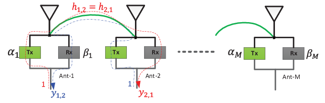
In this paper, we endeavor to find the optimal interconnection strategy or wiring at the BS such that different antennas are connected in the most efficient way to enable the best estimates of the calibration coefficients. To proceed with our derivations, we first make the following assumption:

• •

  AS-1: All the transmission lines have the same length and damping, i.e. $h_{p,q}=h$ when the $p$-th antenna and the $q$-th antenna are interconnected.

In practice, when all the transmission lines have the same length, it could become hard to handle from the hardware implementation point of view in massive MIMO systems. For example, some particular wiring methods could lead to excessive meandering of the transmission lines to some antennas [12].

With AS-1, the calibration signal model in (7) can be simplified to

where the matrix $\mathcal{A}$ represents the interconnection. Specifically, it is defined as

From now on, we assume that we have a total number of $(M-1)$ transmission lines to deploy at the BS. From previous discussion, we know this is the least number of transmission lines that can ensure the interconnection strategy is effective. In fact, we have an $M$-vertex connected graph with $(M-1)$ edges. From Theorem $2.1.4$ in [23], we can readily draw the following conclusion: the calibration path of each ordinary antenna is unique in every effective interconnection strategy with $(M-1)$ transmission lines.

Under AS-2, we have $|\alpha_{m}|=a$ and $|\beta_{m}|=b$. Then the Fisher information matrix in (15) can be rewritten as

where $\bm{t}:=[t_{1},...,t_{f-1},t_{f+1},...,t_{M}]^{T}$ and $t_{m}=|\mathcal{C}_{m}|\geq 1$ denotes the number of antennas that are connected to the $m$-th antenna directly. Regarding the interconnection strategy at the BS, we can have the following useful result. The detailed proof of the following proposition is given in Appendix B.

Now, let’s take a look at the star interconnection strategy as shown in Fig. 4, where all the ordinary antennas are connected to the reference antenna. In this case, the Fisher information matrix $\bm{J}(\tilde{\bm{\theta}})$ becomes diagonal since $\bar{\mathcal{A}}=\bm{O}$. Specifically, the Fisher information matrix in (18) becomes

where

If some ordinary antennas are connected to other ordinary antennas, we see $\bar{\mathcal{A}}\neq\bm{O}$ and the Fisher information matrix $\bm{J}(\tilde{\bm{\theta}})$ is not diagonal anymore. Regarding this kind of interconnection strategies at the BS where some ordinary antennas are interconnected together, based on Proposition 2, we further establish the following useful result. See Appendix C for the proof.

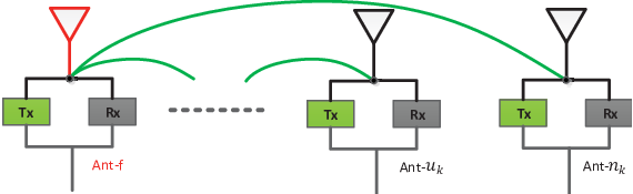
In Fig. 5 and Fig. 6, we have illustrated the aforementioned update in Proposition 3. By taking inverse of both sides of (21), we have the relationship between the CRLBs of the interconnection strategies $\mathcal{A}^{(k)}$ and $\mathcal{A}^{(k+1)}$, i.e.

Note that the CRLB matrix is updated in the reversed order in (24). Specifically, the matrix $(\bm{J}^{(k)}(\tilde{\bm{\theta}}))^{-1}$ is updated with the matrix $(\bm{J}^{(k+1)}(\tilde{\bm{\theta}}))^{-1}$.

According to Proposition 2 and Proposition 3, given the original interconnection strategy $\mathcal{A}^{(0)}$ where $W$ ($W\in[1,M-2]$) ordinary antennas are not interconnected to the reference antenna, we can obtain $\bm{J}^{(k)}(\tilde{\bm{\theta}})$ by applying $k$ appropriate updates as shown in (21). Note that in the interconnection strategy $\mathcal{A}^{(k)}$, there are only $(W-k)$ ordinary antennas which are not interconnected to the reference antenna. Hence, after $W$ updates, the strategy $\mathcal{A}^{(W)}$ becomes the star interconnection strategy since each antenna is interconnected to the reference antenna in $\mathcal{A}^{(W)}$. In other words, after a series of elementary transformations, we will end up with $\bm{J}^{(W)}(\tilde{\bm{\theta}})=\bm{J}_{\text{star}}(\tilde{\bm{\theta}})$, which corresponds to the star interconnection strategy as shown in Fig. 4. Specifically, we have

By taking inverse of both sides of (25), we further obtain

From the result in (26), we can establish the following proposition and the proof is outlined in Appendix D.

From Proposition 4, it can be observed that the CRLBs for the unknown parameters $\alpha_{m}$ and $\beta_{m}$ are directly determined by the calibration path of the $m$-th antenna and the SNR in the corresponding calibration measurement. Furthermore, Proposition 4 provides nice closed-form results for an arbitrary interconnection strategy. For example, when the BS implements the daisy chain interconnection strategy [12] as shown in Fig. 7, where antenna-$m$ and antenna-$(m+1)$ are interconnected, $\forall m\in[1,M-1]$, we have $d_{1}=d_{5}=1$ and $d_{2}=d_{4}=0$. Then the corresponding CRLBs can be computed readily according to (27).

In [12], the authors have shown the daisy chain interconnection strategy would suffer from an error propagation effect assuming noisy calibration measurements. In Proposition 4, we indeed show the error propagation effect on the calibration performance for any effective interconnection strategy with $(M-1)$ transmission lines. Specifically, the CRLBs in (27) indicate that, when the calibration path of the $m$-th ordinary antenna consists of more antennas, the calibration performance will decrease accordingly.

From Proposition 4, we can also easily draw the conclusion that the minimum CRLB is obtained when $d_{m}=0$, $\forall m\neq f$. Obviously, the star interconnection strategy as shown in Fig. 4 can achieve the minimum total CRLB for the calibration coefficients, i.e.

Summarizing we can put forward the following important corollary.

Corollary 1 shows that the star interconnection strategy can achieve the minimum total CRLB for full calibration during the internal self-calibration. Thus the optimal solution of the optimization problem in (17) is the star interconnection. Clearly, Corollary 1 can serve as a design philosophy for internal self-calibration in massive MIMO. In practice, compared with other interconnection strategies, the star interconnection strategy may consume more time resources for signal exchanges and longer transmission lines to interconnect the antennas.

In previous subsection, we have analyzed the optimal interconnection strategy for full calibration at the BS. In fact, similar results can be obtained in the case of relative calibration as well.

Let $c_{m}:=\beta_{m}/\alpha_{m}$, $m\in[1,M]$, denote the relative calibration coefficients to be estimated. Assume $c_{f}$ is known, i.e. the $f$-th antenna serves as the reference antenna. The CRLBs for the relative calibration coefficients can be obtained from the CRLBs for $\tilde{\bm{\theta}}$ [22]. In particular, we can obtain

where $\bm{c}:=[c_{1},\ldots,c_{f-1},c_{f+1},\ldots,c_{M}]^{T}$, the $\bar{m}$-th entry of $\bm{g}(\tilde{\bm{\theta}})$ is $c_{m}$, i.e. $g_{\bar{m}}(\tilde{\bm{\theta}})=c_{m}={\beta_{m}}/{\alpha_{m}}$, $\forall m\in\left\{1,\ldots,f-1,f+1,\ldots,M\right\}$, and $\bar{m}$ denotes the index of the element $c_{m}$ in $\bm{c}$. Note ${\partial\bm{g}(\tilde{\bm{\theta}})}/{\partial\tilde{\bm{\theta}}}$ in (29) is an $(M-1)$-by-$2(M-1)$ Jacobian matrix whose $\bar{m}$-th row is ${\partial g_{\bar{m}}(\tilde{\bm{\theta}})}/{\partial\tilde{\bm{\theta}}}$. It can be verified that all the other elements are zeros except the ${\bar{m}}$-th element and the $(M+{\bar{m}}-1)$-th element in ${\partial g_{\bar{m}}(\tilde{\bm{\theta}})}/{\partial\tilde{\bm{\theta}}}$. Further, these two non-zero elements are given by

According to the results in (27), the CRLB for the relative calibration coefficients $c_{m}$ can be expressed as

From the closed-form CRLB in (31), we can conclude that the star interconnection strategy is also the optimal interconnection for relative calibration.

From the signal model in (8), the likelihood function of $\bm{Y}$ conditioned on $\bm{\alpha}$ and $\bm{\beta}$ can be written as

where $\xi$ includes those terms that do not depend on the unknown parameters. The ML estimates of the calibration coefficients ${\{\alpha_{m},\beta_{m}\}}_{m=1}^{M}\setminus\{\alpha_{f},\beta_{f}\}$ can be obtained by solving the following bi-convex optimization problem:

We can exploit the proposed recursive algorithm as Algorithm 1 to recover the variables $\bm{\alpha}$ and $\bm{\beta}$. In this algorithm, we put those $s$ antennas whose calibration paths to the reference antenna include $r$ antennas in addition to the reference antenna and itself into the set $\mathcal{U}_{r}=\{r_{1},r_{2},\ldots,r_{s}\}$. Specifically, following the definition of $d_{m}$ in Proposition 4, we see $d_{r_{n}}=r,\forall n\in[1,s]$. Also the variable $p_{n}$ in Algorithm 1 denotes the index of one antenna which is in the calibration path of antenna-$r_{n}$ and interconnected to the antenna-$r_{n}$ directly. In Appendix E, we show that Algorithm 1 can achieve the optimal solution of the problem in (32).

For two special interconnection strategies, we can apply Algorithm 1 and obtain the following ML estimates in closed form.

• •

  Star Interconnection: With calibration measurements in (6), the solution of (32) is given by

  $$\begin{split}\hat{\alpha}_{m}=\frac{y_{f,m}}{h\beta_{f}},\ \hat{\beta}_{m}=\frac{y_{m,f}}{h\alpha_{f}},\end{split}$$

  (33)

  where $m\in\{1,2,\ldots,M\}\setminus\{f\}$. Note the corresponding mean square errors (MSEs) of the estimates in (33) are equal to the CRLB results in (27), i.e.

  $$\begin{split}{\sf MSE}(\alpha_{m}):={\sf E}\left[(\hat{\alpha}_{m}-\alpha_{m})^{2}\right]=\frac{\sigma_{n}^{2}}{b^{2}|h|^{2}},\\ {\sf MSE}(\beta_{m}):={\sf E}\left[(\hat{\beta}_{m}-\beta_{m})^{2}\right]=\frac{\sigma_{n}^{2}}{a^{2}|h|^{2}};\end{split}$$

  (34)

• •

  Daisy Chain Interconnection: With this interconnection strategy, the ML estimates can be derived recursively as

  $$\begin{split}\hat{\alpha}_{m}&=\left\{\begin{array}[]{cc}\frac{y_{m+1,m}}{h\hat{\beta}_{m+1}}&m<f\\ \frac{y_{m-1,m}}{h\hat{\beta}_{m-1}}&m>f\end{array}\right.,\\ \hat{\beta}_{m}&=\left\{\begin{array}[]{cc}\frac{y_{m,m+1}}{h\hat{\alpha}_{m+1}}&m<f\\ \frac{y_{m,m-1}}{h\hat{\alpha}_{m-1}}&m>f\end{array}\right.,\end{split}$$

  (35)

  where $\hat{\alpha}_{f}=\alpha_{f}$ and $\hat{\beta}_{f}=\beta_{f}$.

We can rewrite the signal model in (7) as

where $\bm{C}:={\sf Diag}\left\{c_{1},c_{2},\ldots,c_{M}\right\}$, $c_{m}=\beta_{m}/\alpha_{m}$, and $\bm{\Psi}:=\bm{T}\bm{H}\bm{T}$. Similar to the full calibration in Section V-A, the ML estimates for the relative calibration coefficients $\{c_{m}\}_{m=1}^{M}\setminus\{c_{f}\}$ can be obtained by solving the following optimization problem [15]:

With the same notations as in Algorithm 1 for full calibration, we can exploit Algorithm 2 to derive the relative calibration coefficients. In Appendix F, we also show that Algorithm 2 indeed gives the optimal solution of (37). In Algorithm 2, we can see we do not require all the calibration channels to be the same for relative calibration. Moreover, we do not need to know the exact values of $h_{p,q}$. This feature has been exploited in a lot of previous research works, e.g. [18, 9, 15, 12, 16].

For two special interconnection strategies, by applying Algorithm 2, we have the following closed-form results.

• •

  Star Interconnection: For star interconnection, the solution to (37) is given by

  $$\hat{c}_{m}=\frac{y_{m,f}}{y_{f,m}}c_{f},$$

  (38)

  where $m\in\{1,2,\ldots,M\}\setminus\{f\}$;

• •

  Daisy Chain Interconnection: For daisy chain interconnection, the relative calibration coefficients can be estimated recursively as

  $$\begin{split}\hat{c}_{m}=\left\{\begin{array}[]{cc}\frac{y_{m,m+1}}{y_{m+1,m}}\hat{c}_{m+1}&m<f\\ \frac{y_{m,m-1}}{y_{m-1,m}}\hat{c}_{m-1}&m>f\end{array}\right.,\end{split}$$

  (39)

  where $\hat{c}_{f}=c_{f}$.

In [12], the authors have also exploited similar recursive algorithms to acquire the calibration coefficients. But they only considered the star interconnection and the daisy interconnection. On the other hand, our proposed recursive algorithms are more general and can efficiently solve the ML problem for an arbitrary effective interconnection strategy. Besides, we have shown that the recursive algorithms indeed generate the ML estimates.

References

- [1] E. G. Larsson, O. Edfors, F. Tufvesson, and T. L. Marzetta, “Massive MIMO for next generation wireless systems,” IEEE Commun. Mag., vol. 52, no. 2, pp. 186–195, Feb. 2014.
- [2] L. Lu, G. Y. Li, A. L. Swindlehurst, A. Ashikhmin, and R. Zhang, “An overview of massive MIMO: Benefits and challenges,” IEEE J. Sel. Topics Signal Process., vol. 8, no. 5, pp. 742–758, Oct. 2014.
- [3] F. Rusek, D. Persson, B. K. Lau, E. G. Larsson, T. L. Marzetta, O. Edfors, and F. Tufvesson, “Scaling up MIMO: Opportunities and challenges with very large arrays,” IEEE Signal Process. Mag., vol. 30, no. 1, pp. 40–60, Jan. 2013.
- [4] G. S. Smith, “A direct derivation of a single-antenna reciprocity relation for the time domain,” IEEE Trans. Antennas Propag., vol. 52, no. 6, pp. 1568–1577, Jun. 2004.
- [5] B. C. Ng and C. M. S. See, “Sensor-array calibration using a maximum-likelihood approach,” IEEE Trans. Antennas Propag., vol. 44, no. 6, pp. 827–835, Jun. 1996.
- [6] H. Liu, L. Zhao, Y. Li, X. Jing, and T. K. Truong, “A sparse-based approach for DOA estimation and array calibration in uniform linear array,” IEEE Sensors J., vol. 16, no. 15, pp. 6018–6027, Aug. 2016.
- [7] X. Luo, “Multiuser massive MIMO performance with calibration errors,” IEEE Trans. Wireless Commun., vol. 15, no. 7, pp. 4521–4534, Jul. 2016.
- [8] W. Zhang, H. Ren, C. Pan, M. Chen, R. C. Lamare, B. Du, and J. Dai, “Large-scale antenna systems with UL/DL hardware mismatch: achievable rates analysis and calibration,” IEEE Trans. Commun., vol. 63, no. 4, pp. 1216–1229, Apr. 2015.
- [9] H. Wei, D. Wang, H. Zhu, J. Wang, S. Sun, and X. You, “Mutual coupling calibration for multiuser massive MIMO systems,” IEEE Trans. Wireless Commun., vol. 15, no. 1, pp. 606–619, Jan. 2016.
- [10] M. Petermann, M. Stefer, F. Ludwig, D. Wübben, M. Schneider, S. Paul, and K. Kammeyer, “Multi-user pre-pocessing in multi-antenna OFDM TDD systems with non-reciprocal transceivers,” IEEE Trans. Commun., vol. 61, no. 9, pp. 3781–3793, Sep. 2013.
- [11] C. Shepard, H. Yu, N. Anand, L. E. Li, T. Marzetta, R. Yang, and L. Zhong, “Argos: Practical many-antenna base stations,” in Proc. ACM Int. Conf. Mobile Comput. Netw. (Mobicom), Istanbul, Turkey, Aug. 2012, pp. 1–12.
- [12] A. Benzin and G. Caire, “Internal self-calibration methods for large scale array transceiver software-defined radios,” in Proc. IEEE Int. ITG Workshop Smart Antennas, Berlin, Germany, Mar. 2017, pp. 1–8.
- [13] K. Nishimori, K. Cho, Y. Takatori, and T. Hori, “Automatic calibration method using transmitting signals of an adaptive array for TDD systems,” IEEE Trans. Veh. Technol., vol. 50, no. 6, pp. 1636–1640, Nov. 2001.
- [14] J. Liu, G. Vandersteen, J. Craninckx, M. Libois, M. Wouters, F. Petré, and A. Barel, “A novel and low-cost analog frond-end mismatch calibration scheme for MIMO-OFDM WLANs,” in Proc. IEEE Radio and Wireless Symp., San Diego, CA, Oct. 2006, pp. 219–222.
- [15] J. Vieira, F. Rusek, O. Edfors, S. Malkowsky, L. Liu, and F. Tufvesson, “Reciprocity calibration for massive MIMO: Proposal, Modeling, and Validation,” IEEE Trans. Wireless Commun., vol. 16, no. 5, pp. 3042–3056, May 2017.
- [16] F. Kaltenberger, H. Jiang, M. Guillaud, and R. Knopp, “Relative channel reciprocity calibration in MIMO/TDD systems,” in Proc. IEEE Future Netw. Mobile Summit, Florence, Italy, Jun. 2010, pp. 1–10.
- [17] J. Shi, Q. Luo, and M. You, “An efficient method for enhancing TDD over the air reciprocity calibration,” in Proc. IEEE Wireless Commun. Networking Conf., Cancun, Quintana Roo, Mar. 2011, pp. 339–344.
- [18] R. Rogalin, O. Y. Bursalioglu, H. Papadopoulos, G. Caire, A. F. Molisch, A. Michaloliakos, V. Balan, and K. Psounis, “Scalable synchronizaiton and reciprocity calibration for distributed multiuser MIMO,” IEEE Trans. Wireless Commun., vol. 13, no. 4, Apr. 2014.
- [19] X. Luo, “Robust large scale calibration for massive MIMO,” in Proc. IEEE Global Commun. Conf. (GLOBECOM), San Diego, CA, Dec. 2015, pp. 1–6.
- [20] K. Nishimori, T. Hiraguri, T. Ogawa, and H. Yamada, ”Effectiveness of implicit beamforming using calibration technique in massive MIMO system,” in Proc. IEEE Int. Workshop Electromagn. (iWEM), Sapporo, Japan, Aug. 2014, pp. 117–118.
- [21] H. Bolcskei, D. Gesbert, and A. J. Paulraj, “On the capacity of OFDM based spatial multiplexing systems,” IEEE Trans. Commun., vol. 50, no. 2, pp. 225–234, Feb. 2002.
- [22] S. M. Kay, Fundamentals of Statistical Signal Processing: Estimation Theory. Upper Saddle River, New Jersey, USA: Prentice Hall, 1993.
- [23] D. B. West, Introduction to Graph Theory, 2nd ed. Upper Saddle River, NJ, USA: Prentice Hall, 2001.