跳到论文正文
W Papers独立论文阅读器 arXiv:1709.07157 论文正文 计算阅读时间 · 0%
引用这篇论文根据当前论文元数据生成,正式投稿前建议核对。


License: arXiv.org perpetual non-exclusive license
arXiv:1709.07157v1 [math.DS] 21 Sep 2017

Shear flow dynamics
in the Beris-Edwards model of nematic liquid crystals

Adrian C. Murza, Antonio E. Teruel and Arghir D. Zărnescu Address: Adrian C. Murza,
Institute of Mathematics “Simion Stoilow” of the Romanian Academy, Calea Griviţei 21, 010702 Bucharest, Romania
Email address: adrian_murza@hotmail.com Address: Antonio E. Teruel,
Departament de Matemàtiques i Informàtica, Universitat de les Illes Balears, Crta. de Valldemossa km. 7.5, 07122 Palma de Mallorca, Spain
Email address: antonioe.teruel@uib.es Address: Arghir D. Zărnescu
IKERBASQUE, Basque Foundation for Science, Maria Diaz de Haro 3, 48013, Bilbao, Bizkaia, Spain
Address: BCAM, Basque Center for Applied Mathematics, Mazarredo 14, E48009 Bilbao, Bizkaia, Spain Address: “Simion Stoilow” Institute of the Romanian Academy, 21 Calea Griviţei, 010702 Bucharest, Romania Email address: azarnescu@bcamath.org
Abstract.

We consider the Beris-Edwards model describing nematic liquid crystal dynamics and restrict to a shear flow and spatially homogeneous situation. We analyze the dynamics focusing on the effect of the flow. We show that in the co-rotational case one has gradient dynamics, up to a periodic eigenframe rotation, while in the non-co-rotational case we identify the short and long time regime of the dynamics. We express these in terms of the physical variables and compare with the predictions of other models of liquid crystal dynamics.

1. Introduction

Liquid crystals are a mysterious material that is still poorly understood at a basic, fundamental level, despite its impressive technological applications, particularly in liquid crystal displays. It is a material that flows like a liquid, yet it has some properties specific to solids, such as optical properties, that are revealed for instance when passing polarised light through it.

There exist several models that compete in attempting to provide a description at the continuum level. The most comprehensive models regard the material as a complex non-Newtonian fluid, hence they use a Navier-Stokes equation describing the average velocity of the molecules, coupled with a reaction-diffusion-convection equation describing roughly the evolution of the directions of the anisotropic molecules. As such its study is mostly related to fluid mechanics. However, because of the presence of the Navier-Stokes equations the qualitative behaviours of the model are in general very difficult to understand.

On the other hand materials scientists are interested in features of the material relevant in regimes that do not involve significantly its flow behaviour, as it is the case for instance in liquid crystal displays. Thus they study simplified models obtained most often by formally dropping the flow out of the previously mentioned complex fluid equations. The simplified models are easier to understand particularly from the point of view of obtaining qualitative predictions.

However, it is not clear in general what is lost through this simplification and to what extent the presence of the flow significantly affects the dynamics. One setting in which one can understand the presence of the flow, widely used in the engineering studies, and in the rheological literature in determining various properties of liquid crystals, is to consider the effect of a shear flow. This is a rather well behaved flow, for which the Navier-Stokes system simplifies dramatically, yet it produces non trivial effects. Intuitively this simplification allows to describe the local behaviour of the system near a non-singular point of the velocity.

There exist several types of liquid crystals, but we will consider just the simplest and most used in practice, the nematic liquid crystals. For these we use a model well studied in the recent years [1, 3, 5, 13], that combines analytical tractability with physical relevance, namely the Beris-Edwards model. It is a system for the unknowns 𝐮⁡(x,t):ℝ3×(0,+∞)→ℝ3\mathbf{u}(x,t):\mathbb{R}^{3}\times(0,+\infty)\rightarrow\mathbb{R}^{3} representing the incompressible fluid velocity field (of the liquid crystal molecules) and Q⁡(x,t):ℝ3×(0,+∞)→𝒮0(3)Q(x,t):\mathbb{R}^{3}\times(0,+\infty)\rightarrow\mathcal{S}_{0}^{(3)} standing for the order parameter of liquid crystal molecules, where we denote by 𝒮0(3)\mathcal{S}_{0}^{(3)} the QQ-tensor space

𝒮0(3):={Q∈ℝ3×3|Qi​j=Qj​i,∀1≤i,j≤3,tr(Q)=0}.\mathcal{S}_{0}^{(3)}:=\big\{Q\in\mathbb{R}^{3\times 3}|\,Q^{ij}=Q^{ji},\,\forall 1\leq i,j\leq 3,\,\mathrm{tr}(Q)=0\big\}.

Then the Beris-Edwards system, in non-dimensional form, is:

𝐮t+(𝐮⋅∇)𝐮−νΔ𝐮+∇P=\displaystyle\mathbf{u}_{t}+(\mathbf{u}\cdot\nabla)\mathbf{u}-\nu\Delta\mathbf{u}+\nabla{P}= L∇⋅(QΔQ−ΔQQ)−L∇⋅(∇Q⊙∇Q)\displaystyle L\nabla\cdot(Q\Delta{Q}-\Delta{Q}Q)-L\nabla\cdot(\nabla{Q}\odot\nabla{Q})
−ξL∇⋅(ΔQ(Q+13Id)+(Q+13Id)ΔQ−2(Q+13Id)(Q:ΔQ))\displaystyle-\xi L\nabla\cdot\bigg(\Delta Q(Q+\frac{1}{3}Id)+(Q+\frac{1}{3}Id)\Delta Q-2(Q+\frac{1}{3}Id)(Q:\Delta Q)\bigg)
−2ξ∇⋅((Q+13Id)(∂F∂Q:Q−∂F∂Q))\displaystyle-2\xi\nabla\cdot\bigg(\big(Q+\frac{1}{3}\mathrm{Id}\big)(\frac{\partial F}{\partial Q}:Q-\frac{\partial F}{\partial Q})\bigg)
∇⋅𝐮\displaystyle\nabla\cdot\mathbf{u} =0,\displaystyle=0,

where we denoted A:B:=tr​(A​B)A:B:=\textrm{tr}(AB) and I​dId is the 3×33\times 3 identity matrix. This is an equation for the flow 𝐮\mathbf{u} representing the local average velocity of the centers of mass of the rod-like molecules. It is a Navier-Stokes equations with an additional stress tensor encoding the non-Newtonian effect that the interaction of the particles has on their motion.

On the other hand the local orientation of the molecules, represented by QQ, is transported by the flow, rotated and aligned by the flow, and also driven by the bulk free energy FF of the molecules as well as being subjected to Brownian motion:

Qt+(𝐮⋅∇)Q=\displaystyle Q_{t}+(\mathbf{u}\cdot\nabla)Q= (ξ​D+W)​(Q+13​I​d)+(Q+13​I​d)​(ξ​D−W)\displaystyle(\xi D+W)\big(Q+\frac{1}{3}Id\big)+\big(Q+\frac{1}{3}Id\big)(\xi D-W)
−2ξ(Q+13Id)tr(Q∇𝐮)+Γ(LΔQ−∂F∂Q).\displaystyle-2\xi\big(Q+\frac{1}{3}Id\big)\mathrm{tr}(Q\nabla\mathbf{u})+\Gamma\left(L\Delta{Q}-\frac{\partial F}{\partial Q}\right).

where F:=a2​tr​(Q2)−b3​tr​(Q3)+c4​tr2​(Q2)F:=\frac{a}{2}\mathrm{tr}(Q^{2})-\frac{b}{3}\mathrm{tr}(Q^{3})+\frac{c}{4}\mathrm{tr}^{2}(Q^{2}) and

(1) ∂F⁡(Q)∂Q=a​Q−b⁡(Q2−13​I​d​|Q|2)+c​Q​|Q|2\frac{\partial F(Q)}{\partial Q}=aQ-b(Q^{2}-\frac{1}{3}Id|Q|^{2})+cQ|Q|^{2}

is its gradient in 𝒮0(3)\mathcal{S}_{0}^{(3)} (with the term −13​I​d​|Q|2-\frac{1}{3}Id|Q|^{2} representing a Lagrange multiplier accounting for the trace-free constraint). The parameters b,cb,c represent material-dependent constants and aa depends on material and temperature. We will assume throughout the following restrictions (see [12] ):

b,c>0,b2−24​a​c>0b,c>0,b^{2}-24ac>0

The matrices D:=∇𝐮+∇T𝐮2D:=\dfrac{\nabla\mathbf{u}+\nabla^{T}\mathbf{u}}{2}, W:=∇𝐮−∇T𝐮2W:=\dfrac{\nabla\mathbf{u}-\nabla^{T}\mathbf{u}}{2} denote the symmetric and skew-symmetric parts of the velocity matrix, respectively. The coefficient a∈ℝa\in\mathbb{R} is material and temperature dependent, while b∈ℝb\in\mathbb{R} and c∈ℝ+c\in\mathbb{R}_{+} are only material dependent, see [12]. The parameter ξ\xi is related to the aspect ratio of the liquid crystal molecules and heuristically speaking it quantifies the ratio between two effects that the flow has on the liquid crystal molecules: the rotating effect, related to the term [W,Q][W,Q] and the aligning effect that is related to the terms with ξ\xi in front.

We restrict now by taking 𝐮⁡(x,y,z)=(2​y,0,0)\mathbf{u}(x,y,z)=(2y,0,0) to be a shear flow and QQ homogeneous in space. This setting is often considered in the rheological literature and captures the statistical aspects of the flow, in particular combining the dynamical aspects with the phase transitions effects that the nonlinearity in QQ is capable to describe. Then we have:

(2) W=(010−100000)D=(010100000),W=\left(\begin{array}[]{ccc}0&1&0\\ -1&0&0\\ 0&0&0\end{array}\right)\hskip 56.9055ptD=\left(\begin{array}[]{ccc}0&1&0\\ 1&0&0\\ 0&0&0\end{array}\right),

the equation for 𝐮\mathbf{u} is trivially satisfied (with P≡0P\equiv 0) while the equation for QQ reduces to (where we will take for simplicity Γ=1\Gamma=1):

dd​t​Q\displaystyle\frac{d}{dt}Q =[W,Q]+ξ⁡[D​Q+Q​D]+2​ξ3​D−2​ξ​(Q+13​I​d)​tr​[Q​D]−∂F⁡(Q)∂Q\displaystyle=[W,Q]+\xi[DQ+QD]+\frac{2\xi}{3}D-2\xi\left(Q+\frac{1}{3}Id\right)\mathrm{tr}[QD]-\frac{\partial F(Q)}{\partial Q}
(3) =[W,Q]+ξ⁡[D​Q+Q​D]+2​ξ3​D−2​ξ​(Q+13​I​d)​tr​[Q​D]−(a​Q−b⁡(Q2−13​I​d​|Q|2)+c​Q​|Q|2)\displaystyle=[W,Q]+\xi[DQ+QD]+\frac{2\xi}{3}D-2\xi\left(Q+\frac{1}{3}Id\right)\mathrm{tr}[QD]-\left(aQ-b(Q^{2}-\frac{1}{3}Id|Q|^{2})+cQ|Q|^{2}\right)

with [W,Q][W,Q] denoting the commutator of WW and QQ, i.e. [W,Q]=W​Q−Q​W[W,Q]=WQ-QW. We assume without loss of generality that our model has been non-dimensionalised (which can be done in a standard way, completely analogously as in [2]) so all of our parameters are non-dimensional.

It is worth comparing the above equation with the shear-flow model considered for instance in [2, 6]:

(4) dd​t​Q¯=δ⁡([W,Q]+γ​D)−∂F⁡(Q)∂Q\begin{array}[]{l}\displaystyle{\frac{d}{dt}\bar{Q}=\delta([W,Q]+\gamma D)-\frac{\partial F(Q)}{\partial Q}}\end{array}

It was shown in [2, 6] that the model predicts a certain anomalous nongeneric continua of equilibria, the existence of these continua shows that the model is structurally unstable. Our model is more nonlinear and will present a physically more realistic behaviour, in particular it will be seen that asymptotically the effect of the flow disappears and one obtains evolutions towards the steady state of the case without flow.

In our case the major difference it between the case when ξ=0\xi=0 and ξ≠0\xi\not=0. The case ξ=0\xi=0 is called in the literature the “co-rotational case” and is known to be much simpler. In fact we will see that it amounts to a combination of rotation in time and gradient flow behaviour. More precisely the flow will rotate the eigenframe of the matrices with an explicit rate of rotation while the non-trivial dynamics will occur just at the level of eigenvalues but not at the level of eigenframe.

The case ξ≠0\xi\not=0 is much more complex and is responsible with an extraordinary increase in the complexity of the dynamics. As such we will focus on understanding too asymptotic regimes, the short-time and the long-time regimes. It turns out that these are related to the size of ξ\xi in a certain sense, to be detailed later.

The paper is organised as follows: in Section 22 we consider the co-rotational case (ξ=0\xi=0) and we will show that one can completely understand the dynamics and in particular obtain periodic in time solutions. In Section 33 we will analyze the non-corotational case and focus on the short and long time regimes. We will see that we can obtain the phase portrait of the short time regime, while the long time dynamics reduce to evolution towards the manifold of stationary states (of the case without flow). In Section 44 we discuss the results previously obtained in terms of the usual physical variables (scalar order parameters and the director) while commenting on their relevance and the degeneracies one has using them. Finally in Section 55 we provide a conclusion summarising the results thus obtained.

Notations and conventions: We denote by diag​(a,b,c)\textrm{diag}(a,b,c) the three-by-three diagonal matrix with elements a,ba,b and cc (from top to bottom line). For n,m∈ℝ3n,m\in\mathbb{R}^{3} we let n⊗nn\otimes n to be the three-by-three matrix with ni​mjn_{i}m_{j} as the i​jij-th component. We denote by I​dId the three-by-three identity matrix and by I​d2=e1⊗e1+e2⊗e2Id_{2}=e_{1}\otimes e_{1}+e_{2}\otimes e_{2} where e1=(1,0,0),e2=(0,1,0)e_{1}=(1,0,0),e_{2}=(0,1,0).

For two three-by-three matrices AA and BB we take the scalar product in the space of matrices to be A:B=tr⁡(Bt​A)A:B=\mathrm{tr}(B^{t}A) which produces the “Frobenius norm”: |A|=tr​(A2)|A|=\sqrt{\textrm{tr}(A^{2})}.

2. The co-rotational case (ξ=0\xi=0): gradient dynamics and their “rotated” version

In this section we restrict ourselves to studying the case ξ=0\xi=0, which is a limit case, in which the dynamics simplify significantly. In this case the equation (3) becomes

(5) dd​t​Q=[W,Q]−∂F⁡(Q)∂Q=[W,Q]−(a​Q−b⁡(Q2−13​I​d​|Q|2)+c​Q​|Q|2)\begin{array}[]{l}\displaystyle{\frac{d}{dt}Q=[W,Q]-\frac{\partial F(Q)}{\partial Q}}=[W,Q]-\left(aQ-b(Q^{2}-\frac{1}{3}Id|Q|^{2})+cQ|Q|^{2}\right)\end{array}

Then we have that up to a time dependent rotation of the eigenvectors, the dynamics involve just the evolution of eigenvalues. More precisely we have the following:

Proposition 2.1.

Consider the equation (5) where a,b∈ℝa,b\in\mathbb{R} and c∈ℝ+c\in\mathbb{R}_{+}, with WW as defined in (2). Then letting B⁡(t)=eW​t=(cos⁡tsin⁡t0−sin⁡tcos⁡t0000)B(t)=e^{Wt}=\left(\begin{array}[]{lll}\cos t&\sin t&0\\ -\sin t&\cos t&0\\ 0&0&0\end{array}\right) and denoting U⁡(t):=Bt​(t)​Q​(t)​B​(t)U(t):=B^{t}(t)Q(t)B(t) we have that UU is a solution of the gradient flow system:

(6) dd​t​U=−∂F⁡(U)∂U\begin{array}[]{l}\displaystyle{\frac{d}{dt}U=-\frac{\partial F(U)}{\partial U}}\end{array}

for which all ω\omega-limit points belong to the set of stationary points.

Thus for any initial data Q0∈𝒮0(3)Q_{0}\in\mathcal{S}_{0}^{(3)} there exists sequences (tk)k∈ℕ(t_{k})_{k\in\mathbb{N}} with tk→∞t_{k}\to\infty and s∈{0,b+b2−24​a​c4​c,b−b2−24​a​c4​c}s\in\{0,\frac{b+\sqrt{b^{2}-24ac}}{4c},\frac{b-\sqrt{b^{2}-24ac}}{4c}\} (depending on Q0Q_{0} and the time sequence) such that

limtk→∞|Q⁡(tk)−s⁡(n⁡(tk)⊗n⁡(tk)−13​I​d)|=0\lim_{t_{k}\to\infty}|Q(t_{k})-s\left(n(t_{k})\otimes n(t_{k})-\frac{1}{3}Id\right)|=0

with n⁡(t)=(n1​cos⁡t+n2​sin⁡t,−n1​sin⁡t+n2​cos⁡t,0)n(t)=(n_{1}\cos t+n_{2}\sin t,-n_{1}\sin t+n_{2}\cos t,0) for some n12+n22≤1n_{1}^{2}+n_{2}^{2}\leq 1 .

Moreover, if {n,m,p}\{n,m,p\} are an orthonormal family of eigenvectors of Q0Q_{0} then {B⁡(t)​n,B⁡(t)​m,B⁡(t)​p}\{B(t)n,B(t)m,B(t)p\} are an orthonormal family of eigenvectors of Q⁡(t)Q(t), for any t≥0t\geq 0.

Proof.

We introduce the rotation operators B:ℝ→O⁡(3)B:\mathbb{R}\to O(3) as the solution of the system:

(7) {dd​t​B​(t)=W​B​(t)B⁡(0)=I​d\left\{\begin{array}[]{l}\frac{d}{dt}B(t)=WB(t)\\ B(0)=Id\end{array}\right.

In order to see that B⁡(t)∈O⁡(3)B(t)\in O(3) for all t≥0t\geq 0 we note that we have: dd​t​Bt​(t)=−Bt​(t)​W\frac{d}{dt}B^{t}(t)=-B^{t}(t)W. Denoting M⁡(t):=B⁡(t)​Bt​(t)M(t):=B(t)B^{t}(t) we see that M⁡(t)M(t) is a solution of the ODE system dd​t​M=W​M−M​W\frac{d}{dt}M=WM-MW with M⁡(0)=I​dM(0)=Id. Noting that I​dId is a solution of this system, by uniqueness we have M⁡(t)=I​dM(t)=Id for all t≥0t\geq 0. In fact, one can check that we have B⁡(t)=eW​t=(cos⁡tsin⁡t0−sin⁡tcos⁡t0000)B(t)=e^{Wt}=\left(\begin{array}[]{lll}\cos t&\sin t&0\\ -\sin t&\cos t&0\\ 0&0&0\end{array}\right).

We further denote U⁡(t):=Bt​(t)​Q​(t)​B​(t).U(t):=B^{t}(t)Q(t)B(t). Then (5) becomes

dd​t​U​(t)\displaystyle\frac{d}{dt}U(t) =(dd​t​Bt)​Q​B+Bt​(dd​t​Q)​B+Bt​Q​(dd​t​B)=(Bt​(dd​t​Q−W​Q+Q​W)​B)​(t)\displaystyle=(\frac{d}{dt}B^{t})QB+B^{t}(\frac{d}{dt}Q)B+B^{t}Q(\frac{d}{dt}B)=\left(B^{t}\left(\frac{d}{dt}Q-WQ+QW\right)B\right)(t)
=(Bt​(−a​Q+b⁡[Q2−13​|Q|2​I​d]−c​Q​|Q|2)​B)​(t)\displaystyle=\left(B^{t}\left(-aQ+b[Q^{2}-\frac{1}{3}|Q|^{2}Id]-cQ|Q|^{2}\right)B\right)(t)
=(−a​U+b⁡[U2−13​|U|2​I​d]−c​U​|U|2)​(t)\displaystyle=\left(-aU+b[U^{2}-\frac{1}{3}|U|^{2}Id]-cU|U|^{2}\right)(t)
(8) =−∂F⁡(U)∂U\displaystyle=-\frac{\partial F(U)}{\partial U}

hence the equation for UU is a gradient type equation.

We multiply (8) by 2​U2U and take the trace. Denoting α⁡(t):=|U⁡(t)|2\alpha(t):=|U(t)|^{2} we obtain:

(9) α′​(t)=−2​a​α−2​b​tr​(U3)−2​c​α2\alpha^{\prime}(t)=-2a\alpha-2b\textrm{tr}(U^{3})-2c\alpha^{2}

We note that if the matrix UU has eigenvalues λ,μ\lambda,\mu and −λ−μ-\lambda-\mu then α=2​(λ2+μ2+λ​μ)\alpha=2(\lambda^{2}+\mu^{2}+\lambda\mu) and tr​(U3)=−3​λ​μ​(λ+μ)\textrm{tr}(U^{3})=-3\lambda\mu(\lambda+\mu) hence we have:

|tr​(U3)|≤32​(ϵ4​α2+1ϵ​α)|\textrm{tr}(U^{3})|\leq\frac{3}{2}(\frac{\epsilon}{4}\alpha^{2}+\frac{1}{\epsilon}\alpha)

for any ϵ>0\epsilon>0. Using this last relation together with (9) we obtain

α′​(t)≤−2​a​α+3​|b|​(ϵ4​α2+1ϵ​α)−2​c​α2\alpha^{\prime}(t)\leq-2a\alpha+3|b|(\frac{\epsilon}{4}\alpha^{2}+\frac{1}{\epsilon}\alpha)-2c\alpha^{2}

Taking ϵ=4​c3​|b|\epsilon=\frac{4c}{3|b|} and denoting δ:=9​b24​c−2​a\delta:=\frac{9b^{2}}{4c}-2a the last inequality leads to

α′≤δ​α−c​α2≤−|δ|​α+M\alpha^{\prime}\leq\delta\alpha-c\alpha^{2}\leq-|\delta|\alpha+M

where M=(δ−|δ|2​c)2M=\left(\frac{\delta-|\delta|}{2\sqrt{c}}\right)^{2}.

Multiplying by e|δ|​te^{|\delta|t} and integrating over [0,t][0,t] we have:

α⁡(t)≤α⁡(0)​e−|δ|​t+M|δ|\alpha(t)\leq\alpha(0)e^{-|\delta|t}+\frac{M}{|\delta|}

thus the trajectories are bounded, and then the general theory of gradient systems allows to conclude that the limit points are critical points of FF (see for instance [8]). On the other hand it is known (see for instance [11]) that critical points of FF are in the set {s(n⊗n−13Id),n∈𝕊2,s∈{0,b±b2−24​a​c4​c}.\{s\left(n\otimes n-\frac{1}{3}Id\right),\,n\in\mathbb{S}^{2},s\in\{0,\frac{b\pm\sqrt{b^{2}-24ac}}{4c}\}.

We continue by claiming that the dynamics of (6) affects only the eigenvalues, but not the eigenvectors. The argument follows the one in [9] and is presented here for completeness. Indeed, let us consider the system:

d​λd​t\displaystyle\frac{d\lambda}{dt} =−λ⁡[2​c​(λ2+μ2+λ​μ)+a]+b⁡(13​λ2−23​μ2−23​λ​μ),\displaystyle=-\lambda\big[2c(\lambda^{2}+\mu^{2}+\lambda\mu)+a\big]+b\Big(\frac{1}{3}\lambda^{2}-\frac{2}{3}\mu^{2}-\frac{2}{3}\lambda\mu\Big),
(10) d​μd​t\displaystyle\frac{d\mu}{dt} =−μ⁡[2​c​(λ2+μ2+λ​μ)+a]+b⁡(13​μ2−23​λ2−23​λ​μ).\displaystyle=-\mu\big[2c(\lambda^{2}+\mu^{2}+\lambda\mu)+a\big]+b\Big(\frac{1}{3}\mu^{2}-\frac{2}{3}\lambda^{2}-\frac{2}{3}\lambda\mu\Big).

The right hand side of the system is a locally Lipschitz function so the system has a solution locally in time (in fact with some more work global in time and bounded, using arguments similar to the ones before for the matrix system).

On the other hand, let us now take an initial data Q0=diag​(λ0,μ0−λ0−μ0)Q_{0}=\textrm{diag}(\lambda^{0},\mu^{0}-\lambda^{0}-\mu^{0}) and denote Q¯​(t):=diag​(λ⁡(t),μ⁡(t),−λ⁡(t)−μ⁡(t)).\bar{Q}(t):=\textrm{diag}(\lambda(t),\mu(t),-\lambda(t)-\mu(t)). Then, if λ⁡(t),μ⁡(t)\lambda(t),\mu(t) are solutions of (10) with initial data (λ0,μ0)(\lambda^{0},\mu^{0}) then Q¯​(t)\bar{Q}(t) is a solution of (6) with initial data Q0Q_{0}. On the other hand, by uniqueness of solutions of (6), it must be the only solution corresponding to the diagonal initial data Q0Q_{0}. Thus we have shown that a diagonal initial data will generate a diagonal solution.

For an arbitrary, non-diagonal initial data Q~0\tilde{Q}_{0}, since Q~0\tilde{Q}_{0} is a symmetric matrix, there exists a matrix R∈O⁡(3)R\in O(3), such that R​Q~0​Rt=diag​(λ~0,μ~0,−λ~0−μ~0),R\tilde{Q}_{0}R^{t}=\textrm{diag}(\tilde{\lambda}^{0},\tilde{\mu}^{0},-\tilde{\lambda}^{0}-\tilde{\mu}^{0}), where (λ~0,μ~0,−λ~0−μ~0)(\tilde{\lambda}^{0},\tilde{\mu}^{0},-\tilde{\lambda}^{0}-\tilde{\mu}^{0}) are the eigenvalues of Q~0\tilde{Q}_{0}. If Q⁡(t)Q(t) is a solution of (6) with initial data Q~0\tilde{Q}_{0}, then multiplying on the left by the time independent matrix RR, and on the right by the time independent matrix RtR^{t}, using the fact that R​Rt=IdRR^{t}=\mathrm{Id} (as R∈O⁡(3)R\in O(3)), we obtain the following equation:

dd​tRQ(t)Rt=−\displaystyle\frac{d}{dt}RQ(t)R^{t}=- a​R​Q​(t)​Rt+b⁡(R​Q​(t)​Rt​R​Q​(t)​Rt−13​tr​(R​Q​(t)​Rt​R​Q​(t)​Rt)​Id)\displaystyle aRQ(t)R^{t}+b\left(RQ(t)R^{t}RQ(t)R^{t}-\frac{1}{3}\mathrm{tr}(RQ(t)R^{t}RQ(t)R^{t})\mathrm{Id}\right)
−c​R​Q​(t)​Rt​tr​(R​Q​(t)​Rt​R​Q​(t)​Rt).\displaystyle-cRQ(t)R^{t}\mathrm{tr}\big(RQ(t)R^{t}RQ(t)R^{t}\big).

Hence if we denote by M⁡(t):=R​Q​(t)​RtM(t):=RQ(t)R^{t}, we conclude that MM satisfies equation (6) with initial data M0:=R​Q~0​Rt=diag​(λ~0,μ~0,−λ~0−μ~0)M_{0}:=R\tilde{Q}_{0}R^{t}=\textrm{diag}(\tilde{\lambda}^{0},\tilde{\mu}^{0},-\tilde{\lambda}^{0}-\tilde{\mu}^{0}). Since the initial data is diagonal, we infer by previous arguments that M⁡(t)M(t) is diagonal for all times and M⁡(t)=diag​(λ⁡(t),μ⁡(t),−λ⁡(t)−μ⁡(t)),M(t)=\textrm{diag}(\lambda(t),\mu(t),-\lambda(t)-\mu(t)), with λ⁡(t),μ⁡(t)\lambda(t),\mu(t) solutions of (10) with initial data (λ~0,μ~0)(\tilde{\lambda}^{0},\tilde{\mu}^{0}). Thus we obtain that M⁡(t)=R​Q​(t)​Rt=diag​(λ⁡(t),μ⁡(t),−λ⁡(t)−μ⁡(t)),M(t)=RQ(t)R^{t}=\textrm{diag}(\lambda(t),\mu(t),-\lambda(t)-\mu(t)), hence Q⁡(t)=Rt​diag​(λ⁡(t),μ⁡(t),−λ⁡(t)−μ⁡(t))​RQ(t)=R^{t}\textrm{diag}(\lambda(t),\mu(t),-\lambda(t)-\mu(t))R which proves our claim concerning the eingevectors of Q⁡(t)Q(t).

∎

Out of the previous proof one can obtain in particular the existence of solutions that are periodic in time:

Corollary 2.2.

Consider the system (5) with b,c>0b,c>0 and b2−24​a​c>0b^{2}-24ac>0. Let Q0:=s±​(n⊗n−13​I​d)Q_{0}:=s_{\pm}\left(n\otimes n-\frac{1}{3}Id\right) with n∈𝕊2n\in\mathbb{S}^{2} and s±=b±b2−24​a​c4​cs_{\pm}=\frac{b\pm\sqrt{b^{2}-24ac}}{4c}. Then the solution of (5) with initial data Q0Q_{0} is periodic in time and given by:

Q⁡(t)=s±​(n⁡(tk)⊗n⁡(tk)−13​I​d)Q(t)=s_{\pm}\left(n(t_{k})\otimes n(t_{k})-\frac{1}{3}Id\right)

with n⁡(t)=(n1​cos⁡t+n2​sin⁡t,−n1​sin⁡t+n2​cos⁡t,0)n(t)=(n_{1}\cos t+n_{2}\sin t,-n_{1}\sin t+n_{2}\cos t,0).

3. The non-corotational case (ξ≠0\xi\not=0): the short and long time regimes

3.1. Identifying the time regimes: a numerical insight and the magnitude the ξ\xi

We can reprezent QQ in coordinates as

(11) Q:=(xzvzywvw−x−y)Q:=\left(\begin{array}[]{lll}x&z&v\\ z&y&w\\ v&w&-x-y\end{array}\right)

We simplify and take v=w=0v=w=0 (which is a physically relevant regime, see Section 4, consistent with the equations ), and then the system (3) reduces to:

x˙\displaystyle\dot{x} =23​(1−6​x)​z​ξ+2​z−a​x+b3​(x2−2​x​y−2​y2+z2)−2​c​x​(x2+y2+z2+x​y)\displaystyle=\frac{2}{3}(1-6x)z\xi+2z-ax+\frac{b}{3}(x^{2}-2xy-2y^{2}+z^{2})-2cx(x^{2}+y^{2}+z^{2}+xy)
y˙\displaystyle\dot{y} =23​(1−6​y)​z​ξ−2​z−a​y+b3​(−2​x2−2​x​y+y2+z2)−2​c​y​(x2+y2+z2+x​y)\displaystyle=\frac{2}{3}(1-6y)z\xi-2z-ay+\frac{b}{3}(-2x^{2}-2xy+y^{2}+z^{2})-2cy(x^{2}+y^{2}+z^{2}+xy)
(12) z˙\displaystyle\dot{z} =(23+x+y−4​z2)​ξ−x+y−a​z+b⁡(x​z+y​z)−2​c​z​(x2+y2+z2+x​y)\displaystyle=(\frac{2}{3}+x+y-4z^{2})\xi-x+y-az+b(xz+yz)-2cz(x^{2}+y^{2}+z^{2}+xy)

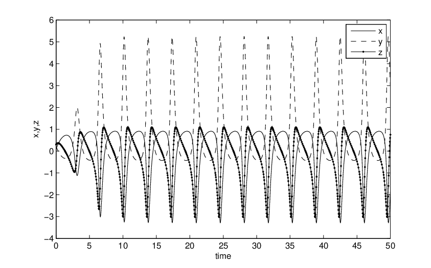
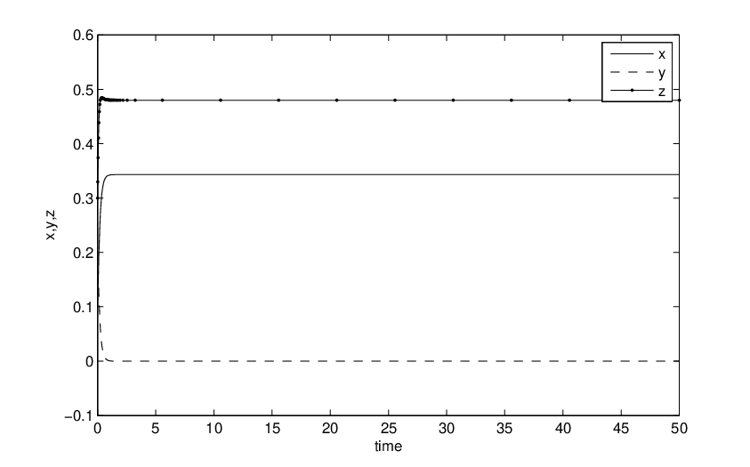
We consider now a couple of simulations, to understand the dynamics provided by this system. These are obtained by taking a=−0.2,b=0.1,c=0.1a=-0.2,b=0.1,c=0.1 and time t=50t=50 but varying ξ\xi.

Refer to caption
Refer to caption
Figure 1. Dynamics for ξ=0.5\xi=0.5 (top) and ξ=3\xi=3 (bottom)

What we obtain is that the dynamics are dramatically different depending on the size of ξ\xi. For small ξ\xi we have essentially dynamics as provided in the co-rotational case, i.e. evolving to periodic solutions, while for large ξ\xi the periodicity is destroyed and we evolve fast towards a steady state.

In order to obtain an analytical inside into this, let us consider the new function:

(13) Qξ​(t):=Q​(tξ)Q_{\xi}(t):=Q(\frac{t}{\xi})

Then QξQ_{\xi} satisfies the system:

dd​t​Qξ=\displaystyle\frac{d}{dt}Q_{\xi}= [D​Qξ+Qξ​D]+23​D−2​(Qξ+13​I​d)​tr​[Qξ​D]+1ξ​([W,Qξ]−∂F∂Q​(Qξ))\displaystyle[DQ_{\xi}+Q_{\xi}D]+\frac{2}{3}D-2\left(Q_{\xi}+\frac{1}{3}Id\right)\mathrm{tr}[Q_{\xi}D]+\frac{1}{\xi}\bigg([W,Q_{\xi}]-\frac{\partial F}{\partial Q}(Q_{\xi})\bigg)
=\displaystyle= [D​Qξ+Qξ​D]+23​D−2​(Qξ+13​I​d)​tr​[Qξ​D]\displaystyle[DQ_{\xi}+Q_{\xi}D]+\frac{2}{3}D-2\left(Q_{\xi}+\frac{1}{3}Id\right)\mathrm{tr}[Q_{\xi}D]
(14) +1ξ​([W,Qξ]−a​Qξ+b⁡(Qξ2−13​|Qξ|2​I​d)−c​Qξ​|Qξ|2)\displaystyle+\frac{1}{\xi}\bigg([W,Q_{\xi}]-aQ_{\xi}+b(Q_{\xi}^{2}-\frac{1}{3}|Q_{\xi}|^{2}Id)-cQ_{\xi}|Q_{\xi}|^{2}\bigg)

Thus we have two regimes:

  • •

    The “short time” regime, when ξ→∞\xi\to\infty. In this case the equation QξQ_{\xi} formally converges on finite intervals to:

    (15) dd​t​R=[D​R+R​D]+23​D−2​(R+13​I​d)​tr​[R​D]\frac{d}{dt}R=[DR+RD]+\frac{2}{3}D-2\left(R+\frac{1}{3}Id\right)\mathrm{tr}[RD]

    Note that as ξ→∞\xi\to\infty we have Q⁡(tξ)→Q⁡(0)Q(\frac{t}{\xi})\to Q(0) so the equation (15) describes the behaviour near the initial time.

  • •

    The “long time” regime, when ξ→0\xi\to 0. In this case the QξQ_{\xi} formally converges to:

    (16) 0=[W,Q]−∂F⁡(Q)∂Q0=[W,Q]-\frac{\partial F(Q)}{\partial Q}

    so one would expect evolution towards a fixed point, solution of this stationary equation.

Remark 1.

It should be noted that one does not obtain through these rescalings a direct understanding of the simulations in Figure 1 which represent evolutions at intermediary times (neither too long, nor too short), unlike in the analytical arguments that will be provided, analyzing asymptotic regimes. However the simulations are useful for showing the complexity of the intermediary time regimes.

3.2. The short time regime

We have the following proposition formalizing the intuition mentioned before:

Proposition 3.1.

Let QξQ_{\xi} be the solution of (14) with Qξ​(0)=Q0Q_{\xi}(0)=Q_{0} and RR the solution of (15) with R⁡(0)=Q0R(0)=Q_{0}. There exists a time T∗T^{*} depending only on |Q0||Q_{0}| but independent of ξ\xi such that the solutions for both (14) and (15) exist on [0,T∗][0,T^{*}] and moreover we have:

(17) limξ→∞supt∈[0,T∗]|Qξ​(t)−R|=0\lim_{\xi\to\infty}\sup_{t\in[0,T^{*}]}|Q_{\xi}(t)-R|=0
Proof.

We start by deriving a uniform local in time estimate for RR. We multiply (15) scalarly by 2​R2R to get:

dd​t​|R|2=4​tr​(R2​D)+43​tr​(D​R)−4​tr​(R​D)​|R|2\frac{d}{dt}|R|^{2}=4\mathrm{tr}(R^{2}D)+\frac{4}{3}\mathrm{tr}(DR)-4\mathrm{tr}(RD)|R|^{2}

Then we have:

dd​t​|R|2≤C1​|R|4+C2​|R|2+C3\frac{d}{dt}|R|^{2}\leq C_{1}|R|^{4}+C_{2}|R|^{2}+C_{3}

where C1,C2,C3>0C_{1},C_{2},C_{3}>0 are explicitly computable coefficients.

Dividing the last estimate by 1+|R|41+|R|^{4} we get:

dd​t​|R|21+|R|4≤C1+C22+C3\frac{\frac{d}{dt}|R|^{2}}{1+|R|^{4}}\leq C_{1}+\frac{C_{2}}{2}+C_{3}

Integrating on [0,t][0,t] we obtain:

|R⁡(t)|2≤|R⁡(0)|2+tan⁡(C4​t)1−|R⁡(0)|2​tan⁡(C4​t)|R(t)|^{2}\leq\frac{|R(0)|^{2}+\tan(C_{4}t)}{1-|R(0)|^{2}\tan(C_{4}t)}

where C4:=C1+C22+C3C_{4}:=C_{1}+\frac{C_{2}}{2}+C_{3}. The estimate is valid for t<T1∗t<T^{*}_{1} depending on R⁡(0)R(0) and C4C_{4}.

Similarly we estimate QξQ_{\xi}. We multiply (14) scalarly by 2​Qξ2Q_{\xi} and obtain:

(18) dd​t​|Qξ|2=4​tr​(Qξ2​D)+43​tr​(D​Qξ)−4​tr​(D​Qξ)​|Qξ|2−2ξ​(a​|Qξ|2−b​tr​(Qξ)3+c​|Qξ|4)\frac{d}{dt}|Q_{\xi}|^{2}=4\mathrm{tr}(Q_{\xi}^{2}D)+\frac{4}{3}\mathrm{tr}(DQ_{\xi})-4\mathrm{tr}(DQ_{\xi})|Q_{\xi}|^{2}-\frac{2}{\xi}\left(a|Q_{\xi}|^{2}-b\mathrm{tr}(Q_{\xi})^{3}+c|Q_{\xi}|^{4}\right)

which implies

dd​t​|Qξ|2\displaystyle\frac{d}{dt}|Q_{\xi}|^{2} ≤4​|Qξ2|​|D|+43​|D||Qξ|−4​t​r​(D​Qξ)​|Qξ|2−2ξ​(a​|Qξ|2−b​tr​(Qξ)3+c​|Qξ|4)\displaystyle\leq 4|Q_{\xi}^{2}||D|+\frac{4}{3}|D||Q_{\xi}|-4\mathrm{tr}(DQ_{\xi})|Q_{\xi}|^{2}-\frac{2}{\xi}\left(a|Q_{\xi}|^{2}-b\mathrm{tr}(Q_{\xi})^{3}+c|Q_{\xi}|^{4}\right)
≤2​|Qξ2|2+2​|D|2+23​|Qξ|2+23​|D|2+2​(tr⁡(D​Qξ))2+2​|Qξ|4−2ξ​(a​|Qξ|2−b​tr​(Qξ)3+c​|Qξ|4)\displaystyle\leq 2|Q_{\xi}^{2}|^{2}+2|D|^{2}+\frac{2}{3}|Q_{\xi}|^{2}+\frac{2}{3}|D|^{2}+2(\mathrm{tr}(DQ_{\xi}))^{2}+2|Q_{\xi}|^{4}-\frac{2}{\xi}\left(a|Q_{\xi}|^{2}-b\mathrm{tr}(Q_{\xi})^{3}+c|Q_{\xi}|^{4}\right)
≤4​|Qξ|4+23​|Qξ|2+113​|D|2+|D|4−2ξ​(a​|Qξ|2−b​tr​(Qξ)3+c​|Qξ|4)\displaystyle\leq 4|Q_{\xi}|^{4}+\frac{2}{3}|Q_{\xi}|^{2}+\frac{11}{3}|D|^{2}+|D|^{4}-\frac{2}{\xi}\left(a|Q_{\xi}|^{2}-b\mathrm{tr}(Q_{\xi})^{3}+c|Q_{\xi}|^{4}\right)
(19) ≤(C~1+C~2ξ)​|Qξ|4+C~3ξ​|Qξ|2+C~4\displaystyle\leq(\tilde{C}_{1}+\frac{\tilde{C}_{2}}{\xi})|Q_{\xi}|^{4}+\frac{\tilde{C}_{3}}{\xi}|Q_{\xi}|^{2}+\tilde{C}_{4}

where we used that |tr⁡(A​B)|≤|A|​|B||\mathrm{tr}(AB)|\leq|A||B| for any 3×33\times 3 matrices, and |M|4=2​|M2|2|M|^{4}=2|M^{2}|^{2} for a Q-tensor, with C~1,C~2,C~3,C~4>0\tilde{C}_{1},\tilde{C}_{2},\tilde{C}_{3},\tilde{C}_{4}>0 explicitly computable constants, where C~2,C~3\tilde{C}_{2},\tilde{C}_{3} depend on the coefficients a,ba,b and cc.

Dividing the last estimate by 1+|Qξ|41+|Q_{\xi}|^{4} we get:

(20) dd​t​|Qξ|21+|Qξ|4≤C~1+1ξ​(C~2+C~32)+C~4\frac{\frac{d}{dt}|Q_{\xi}|^{2}}{1+|Q_{\xi}|^{4}}\leq\tilde{C}_{1}+\frac{1}{\xi}(\tilde{C}_{2}+\frac{\tilde{C}_{3}}{2})+\tilde{C}_{4}

which integrating on [0,t][0,t] gives:

(21) |Qξ|2​(t)≤|Q0|2+tan⁡(C~5,ξ​t)1−|Q0|2​tan⁡(C5​ξ​t)|Q_{\xi}|^{2}(t)\leq\frac{|Q_{0}|^{2}+\tan(\tilde{C}_{5,\xi}t)}{1-|Q_{0}|^{2}\tan(C_{5\xi}t)}

where C~5,ξ=C~1+1ξ​(C~2+C~32)+C~4\tilde{C}_{5,\xi}=\tilde{C}_{1}+\frac{1}{\xi}(\tilde{C}_{2}+\frac{\tilde{C}_{3}}{2})+\tilde{C}_{4} and for t<T2∗t<T^{*}_{2} with T2∗T^{*}_{2} depending on |Qξ​(0)||Q_{\xi}(0)|, C~1,C~4\tilde{C}_{1},\tilde{C}_{4} but independent of ξ\xi.

We now denote Rξ:=Qξ−RR_{\xi}:=Q_{\xi}-R where RR is a solution of the equation (15) with initial data R⁡(0)=Qξ​(0)=Q0R(0)=Q_{\xi}(0)=Q_{0}. We have that RξR_{\xi} satisfies the equation:

dd​t​Rξ=[D​Rξ+Rξ​D]−\displaystyle\frac{d}{dt}R_{\xi}=[DR_{\xi}+R_{\xi}D]- 2​Rξ​tr​(Qξ​D)−23​I​d​tr​(Rξ​D)−2​R​tr​(Rξ​D)\displaystyle 2R_{\xi}\mathrm{tr}(Q_{\xi}D)-\frac{2}{3}Id\mathrm{tr}(R_{\xi}D)-2R\mathrm{tr}(R_{\xi}D)
(22) +1ξ​([W,Qξ]−a​Qξ+b⁡(Qξ2−13​I​d​|Qξ|2)−c​Qξ​|Qξ|2)\displaystyle+\frac{1}{\xi}\bigg([W,Q_{\xi}]-aQ_{\xi}+b(Q_{\xi}^{2}-\frac{1}{3}Id|Q_{\xi}|^{2})-cQ_{\xi}|Q_{\xi}|^{2}\bigg)

Multiplying by 2​Rξ2R_{\xi} and estimating similarly as before we obtain:

(23) dd​t​|Rξ|2≤C¯1​(1+1ξ)​|Rξ|2+C¯2​|Rξ|2​|Qξ|+C¯3​|Rξ|2​|R|+C¯4ξ​(1+|Qξ|6)\frac{d}{dt}|R_{\xi}|^{2}\leq\bar{C}_{1}(1+\frac{1}{\xi})|R_{\xi}|^{2}+\bar{C}_{2}|R_{\xi}|^{2}|Q_{\xi}|+\bar{C}_{3}|R_{\xi}|^{2}|R|+\frac{\bar{C}_{4}}{\xi}(1+|Q_{\xi}|^{6})

where C¯1,C¯2,C¯3,C¯4>0\bar{C}_{1},\bar{C}_{2},\bar{C}_{3},\bar{C}_{4}>0 are explicitly computable constants depending only on DD, WW, a,b,ca,b,c but not on ξ\xi.

Noting that Qξ​(0)=Q0=R⁡(0)Q_{\xi}(0)=Q_{0}=R(0) we have Rξ​(0)=0R_{\xi}(0)=0 and thus using Gronwall inequality we get out of (23) that:

(24) |Rξ|2​(t)≤C¯4ξ​∫0t(1+|Qξ|6)​(s)​exp⁡(∫stC¯1​(1+1ξ)+C¯2​|Qξ|​(τ)+C¯3​|R|​(τ)​𝑑τ)​𝑑s|R_{\xi}|^{2}(t)\leq\frac{\bar{C}_{4}}{\xi}\int_{0}^{t}(1+|Q_{\xi}|^{6})(s)\exp(\int_{s}^{t}\bar{C}_{1}(1+\frac{1}{\xi})+\bar{C}_{2}|Q_{\xi}|(\tau)+\bar{C}_{3}|R|(\tau)\,d\tau)\,ds

Thus, for T<min⁡{T1∗,T2∗}T<\min\{T_{1}^{*},T_{2}^{*}\} we have

(25) supt∈[0,T]|Qξ​(t)−R⁡(t)|→0, as ​ξ→∞\sup_{t\in[0,T]}|Q_{\xi}(t)-R(t)|\to 0,\textrm{ as }\xi\to\infty

∎

3.3. Coordinates and the analysis of the short time regime

In order to describing the initial behaviour more precisely it is convenient to revert to coordinate representation. The system describing the initial behaviour in coordinates is given by:

(26) x˙=23​(1−6​x)​zy˙=23​(1−6​y)​zz˙=23+x+y−4​z2.\begin{array}[]{l}\dot{x}=\displaystyle{\frac{2}{3}}(1-6x)z\\ \\ \dot{y}=\displaystyle{\frac{2}{3}}(1-6y)z\\ \\ \dot{z}=\displaystyle{\frac{2}{3}}+x+y-4z^{2}.\end{array}
Proposition 3.2.

System (26) is integrable in ℝ3∖{x=1/6}\mathbb{R}^{3}\setminus\{x=1/6\} and the two independent first integrals are

(27) ℋ1​(x,y,z):=1−6​y6​(1−6​x)ℋ2​(x,y,z):=1+6​x+6​y−12​z236​(1−6​x)2.\begin{array}[]{l}\mathcal{H}_{1}(x,y,z):=\displaystyle{\frac{1-6y}{6(1-6x)}}\\ \\ \mathcal{H}_{2}(x,y,z):=\displaystyle{\frac{1+6x+6y-12z^{2}}{36(1-6x)^{2}}}.\end{array}
Proof.

The proof follows from straightforward calculations. ∎

Proposition 3.3.

Singular points of system (26) are: every point belonging the straight line

r:={x+y=−2/3,z=0},r:=\left\{x+y=-2/3,\ z=0\right\},

which is non-hyperbolic; and the hyperbolic ones

E2:=(16,16,−12),E3:=(16,16,12),\begin{array}[]{l}E_{2}:=\displaystyle{\left(\frac{1}{6},\frac{1}{6},-\frac{1}{2}\right)},~~E_{3}:=\displaystyle{\left(\frac{1}{6},\frac{1}{6},\frac{1}{2}\right)},\end{array}

where E2E_{2} is a repelling node and E3E_{3} is an attracting node. The planes x+y+2z=−2/3x+y+2z=-2/3 and x+y+2z=−2/3x+y+2z=-2/3 are invariant under the flow and intersect along rr. Moreover, the global phase portrait of system (26) is topologically equivalent to the one represented in Figure 3.

Proof.

The existence of the singularities and the local behaviour of the hyperbolic ones follow from straightforward calculations.

The invariance of the planes in the statement of the proposition follows by checking that

x˙​d​fd​x+y˙​d​fd​y+z˙​d​fd​z=−2​(2​z±1)​f​(x,y,z)\dot{x}\dfrac{df}{dx}+\dot{y}\dfrac{df}{dy}+\dot{z}\dfrac{df}{dz}=-2(2z\pm 1)f(x,y,z)

where f⁡(x,y,z)=x+y−2​z+2/3f(x,y,z)=x+y-2z+2/3 and f⁡(x,y,z)=x+y+2​z+2/3f(x,y,z)=x+y+2z+2/3, respectively.

Let we describe now the global phase portrait. To do that, we first describe the foliation induced by the level surfaces IhI_{h} of the first integral ℋ1\mathcal{H}_{1}, and then to analyze the dynamical behaviour of the restriction of system (26) to IhI_{h}, we use the restriction to IhI_{h} of the other first integral ℋ2\mathcal{H}_{2}.

Note that the invariant surfaces Ih:={(x,y,z):ℋ1​(x,y,z)=h}h∈ℝI_{h}:=\{(x,y,z):\mathcal{H}_{1}(x,y,z)=h\}_{h\in\mathbb{R}}, are the planes given by

(28) y=1/6−h⁡(1−6​x)y=1/6-h(1-6x)

and z∈ℝz\in\mathbb{R}. Moreover, the plane given by x=1/6x=1/6 and z∈ℝz\in\mathbb{R} is also invariant under the flow of system (26), even when it is not a level surface of ℋ1\mathcal{H}_{1}. All these vertical planes intersect along the invariant straight line x=1/6x=1/6, y=1/6y=1/6 and z∈ℝz\in\mathbb{R}.

By replacing expression (28) into the third equation of (26) we obtain

(29) x˙=23​(1−6​x)​zz˙=56+x−4​z2−h⁡(1−6​x),\begin{array}[]{l}\dot{x}=\displaystyle{\frac{2}{3}(1-6x)z}\\ \\ \dot{z}=\displaystyle{\frac{5}{6}+x-4z^{2}-h(1-6x)},\end{array}

which corresponds with the restricted differential system over the invariant manifold IhI_{h}.

If h≠−1/6h\neq-1/6, then it is easy to check that the system (29) has three hyperbolic singular points: one of them

rh=(6​h−56​(1+6​h),0),{r}_{h}=\left(\dfrac{6h-5}{6(1+6h)},0\right),

corresponding with the intersection of the straight line rr and the plane IhI_{h}; and the other two corresponding with E2E_{2} and E3E_{3}, which will be referenced in the same way. Linear analysis around the singularities assures that rhr_{h} is a saddle point, E2E_{2} is a repelling node and E3E_{3} is an attracting node.

For the globaly description of the phase portrait of system (29) we resort to the restriction of the first integral ℋ2\mathcal{H}_{2} to the invariant plane IhI_{h},

ℋ2|h=1+3​x+6​z2−3​h​(1−6​x)18​(1−6​x)2.\left.\mathcal{H}_{2}\right|_{h}=\dfrac{1+3x+6z^{2}-3h(1-6x)}{18(1-6x)^{2}}.

Hence, the level curves of ℋ2|h\left.\mathcal{H}_{2}\right|_{h} containing the singular point rhr_{h}, that is ℋ2|h​(x,z)=ℋ2|h​(rh)\left.\mathcal{H}_{2}\right|_{h}(x,z)=\left.\mathcal{H}_{2}\right|_{h}(r_{h}), are the two invariant straight lines

(5+6​x−12​z−6​h​(1−6​x))​(5+6​x+12​z−6​h​(1−6​x))=0.(5+6x-12z-6h(1-6x))(5+6x+12z-6h(1-6x))=0.

Notice that the first of these lines contains the attracting node E2E_{2} whereas the second one containes the repelling node E3E_{3}. From this, we conclude that the global phase portrait is topological equivalent to the one depicted in Figure 2(a) when h<−1/6h<-1/6 or in Figure 2(c) when h>−1/6h>-1/6.

On the other hand, if h=−1/6h=-1/6, then system (2) exhibits only the singularities which correspond with E2E_{2} and E3E_{3}, having both of them the same local behaviour as before. Moreover, the straight lines

x=16,z=12,and​z=−12,x=\dfrac{1}{6},\ z=\dfrac{1}{2},\ \text{and}\ z=-\dfrac{1}{2},

are invariant under the flow. We conclude that the global phase portrait is topological equivalent to the one depicted in Figure 2(b).

Refer to caption(a) E 2 E 3 r h (b) E 2 E 3 (c) E 2 E 3 r h
Figure 2. Schematic representation of the flow of system (29) in the x​zxz plane, vertical invariant line at x=1/6x=1/6: (a) when h<−1/6h<-1/6; (b) when h=−1/6h=-1/6; and (c) when h>−1/6h>-1/6. Blue orbits correspond with the separatrices.

To finish describing the global behaviour of system (26), it remains to describe the flow over the invariant plane x=1/6x=1/6. This can be done just by notting than the restriction of the system (26) to the plane x=1/6x=1/6 coincides with the system (29), by taking h=0h=0 and performing the change of variable x→yx\to y. Therefore, the flow over the plane x=1/6x=1/6 is topological equivalent to the one depicted in Figure 2(c). ∎

Refer to caption r x + y - 2 z = - 2 / 3 x + y + 2 z = - 2 / 3 = - x y 0 E 3 ⁢ W s ( E 3 ) ⁢ W u ( E 2 ) E 2
Figure 3. Global phase portrait of system (26). The thick line corresponds with the continuum of non-hyperbolic singular points rr, the non-filled circle corresponds with the repelling node E2E_{2} and the filled one with the attracting node E3E_{3}. The gray planes correspond with the invariant surface x+y+2z=−2/3x+y+2z=-2/3, containing E2E_{2} and the invariant surface x+y+2z=−2/3x+y+2z=-2/3, containing E3E_{3}. The first of these planes is the boundary of the stable manifold of E3E_{3}, denoted by Ws​(E3)W^{s}(E_{3}), whereas the second plane is the boundary of the unstable manifold of E2E_{2}, denoted by Wu​(E2)W^{u}(E_{2}). We also represent the planes z=0z=0 and x−y=0x-y=0. These planes have not dynamical meaning, the second one is included just to justify that both half-spaces x−y<0x-y<0 and x−y>0x-y>0 are invariant under the flow, see Remark 2.
Remark 2.

The plane x−y=0x-y=0 is invariant under the flow of system (26) since it corresponds with the level surface I1/6I_{1/6}, see (28). Therefore, both half-spaces x−y<0x-y<0 and x−y>0x-y>0 are also invariant under the flow of system (26).

3.4. The long time regime

We have first an uniform estimate for |Qξ||Q_{\xi}| which uses in an essential manner the fact that the material constant cc appearing in (1) is positive.

Lemma 3.4.

Let QξQ_{\xi} be a solution of (14). There exists C~,ξ0>0\tilde{C},\xi_{0}>0 depending on the material constants a,b,ca,b,c but independent of ξ\xi, such that:

(30) |Qξ|​(t)≤|Qξ|​(0)+C~|Q_{\xi}|(t)\leq|Q_{\xi}|(0)+\tilde{C}

for all t≥0t\geq 0 and ξ<ξ0\xi<\xi_{0}.

Proof.

We multiply (14) by 2​Qξ2Q_{\xi} and we obtain the estimate:

dd​t​|Qξ|2\displaystyle\frac{d}{dt}|Q_{\xi}|^{2} ≤C1​|Qξ|2+C2+C3ξ​|Qξ|2−C4ξ​|Qξ|4\displaystyle\leq C_{1}|Q_{\xi}|^{2}+C_{2}+\frac{C_{3}}{\xi}|Q_{\xi}|^{2}-\frac{C_{4}}{\xi}|Q_{\xi}|^{4}
≤C2+C5ξ−C6ξ​|Qξ|2\displaystyle\leq C_{2}+\frac{C_{5}}{\xi}-\frac{C_{6}}{\xi}|Q_{\xi}|^{2}

for some ξ<ξ0\xi<\xi_{0} and positive explicitly computable constants Ci>0,i=1,…,6C_{i}>0,i=1,\dots,6 depending on a,b,ca,b,c and ξ0\xi_{0} but not on ξ\xi.

Multiplying the last inequality by eC6​tξe^{\frac{C_{6}t}{\xi}} and integrating on [0,t][0,t] we get:

|Qξ|2​(t)≤|Qξ|2​(0)​e−C6​tξ+(C2+C5ξ)​ξC6​(1−e−C6​tξ)\displaystyle{|Q_{\xi}|^{2}(t)\leq|Q_{\xi}|^{2}(0)e^{-\frac{C_{6}t}{\xi}}+\left(C_{2}+\frac{C_{5}}{\xi}\right)\frac{\xi}{C_{6}}\left(1-e^{-\frac{C_{6}t}{\xi}}\right)}

out of which we obtain the claimed estimate (30).

∎

We show now that the long-time behaviour of QQ described by the limit on finite time intervals of QξQ_{\xi} as ξ→0\xi\to 0 is provided by solutions of (16).

Lemma 3.5.

Let QξQ_{\xi} be a solution of (14). We have:

(31) limξ→0∫0t|[W,Qξ]−∂F∂Q​(Qξ)|2​(s)​𝑑s=0\lim_{\xi\to 0}\int_{0}^{t}|[W,Q_{\xi}]-\frac{\partial F}{\partial Q}(Q_{\xi})|^{2}(s)\,ds=0
Proof.

We multiply the equation (14) by ∂F∂Q​(Qξ)−[W,Qξ]\frac{\partial F}{\partial Q}(Q_{\xi})-[W,Q_{\xi}] and obtain:

∂tF⁡(Qξ)\displaystyle\partial_{t}F(Q_{\xi}) =−1ξ​|∂F∂Q​(Qξ)−[W,Qξ]|2\displaystyle=-\frac{1}{\xi}|\frac{\partial F}{\partial Q}(Q_{\xi})-[W,Q_{\xi}]|^{2}
+(∂F∂Q​(Qξ)−[W,Qξ])​([D​Qξ+Qξ​D]+23​D−2​(Qξ+13​I​d)​tr​[Qξ​D])\displaystyle+\left(\frac{\partial F}{\partial Q}(Q_{\xi})-[W,Q_{\xi}]\right)\left([DQ_{\xi}+Q_{\xi}D]+\frac{2}{3}D-2\left(Q_{\xi}+\frac{1}{3}Id\right)\mathrm{tr}[Q_{\xi}D]\right)
(32) ≤−12​ξ​|∂F∂Q​(Qξ)−[W,Qξ]|2+C~​ξ\displaystyle\leq-\frac{1}{2\xi}|\frac{\partial F}{\partial Q}(Q_{\xi})-[W,Q_{\xi}]|^{2}+\tilde{C}\xi

for ξ<ξ0\xi<\xi_{0} (with ξ0\xi_{0} depending on the time tt and the initial data), with C~\tilde{C} independent of ξ0\xi_{0}, where for the last inequality we used the estimate (30). Integrating the last inequality and using the fact that F⁡(Qξ)F(Q_{\xi}) is bounded for bounded QξQ_{\xi} we obtain the claimed relation (31).

∎

We continue by identifying the solutions of the limiting equation (16):

Lemma 3.6.

For the matrix WW as in (2) and ∂F∂Q​(Q)\frac{\partial F}{\partial Q}(Q) as in (1) we have

[W,Q]−∂F∂Q​(Q)=0[W,Q]-\frac{\partial F}{\partial Q}(Q)=0

if and only if

(33) Q∈{0,s±​(n⊗n−13​I​d),i=1,2,3,n∈𝕊2}Q\in\{0,s_{\pm}(n\otimes n-\frac{1}{3}Id),i=1,2,3,n\in\mathbb{S}^{2}\}

with s±:=b±b2−24​a​c4​c\displaystyle{s_{\pm}:=\frac{b\pm\sqrt{b^{2}-24ac}}{4c}}.

Proof.

For a given tensor QQ we take ℛ⁡[Q]∈S​O​(3)\mathcal{R}[Q]\in SO(3) to be such that ℛ⁡[Q]​Q​ℛt​[Q]\mathcal{R}[Q]Q\mathcal{R}^{t}[Q] is a diagonal matrix, say

(34) 𝒟:=ℛ⁡[Q]​Q​ℛt​[Q]=(x000y000−x−y)\mathcal{D}:=\mathcal{R}[Q]Q\mathcal{R}^{t}[Q]=\left(\begin{array}[]{lll}x&0&0\\ 0&y&0\\ 0&0&-x-y\end{array}\right)

with x,y,−x−yx,y,-x-y being eigenvalues of QQ.

We explicitate

ℛ⁡[Q]:=(a11a12a13a21a22a23a31a32a33)\mathcal{R}[Q]:=\left(\begin{array}[]{lll}a_{11}&a_{12}&a_{13}\\ a_{21}&a_{22}&a_{23}\\ a_{31}&a_{32}&a_{33}\end{array}\right)

(note that the coefficients depend on the matrix QQ). Then, denoting

(35) α:=a11​a22−a12​a21,ξ:=a11​a32−a12​a31,γ:=a21​a32−a22​a31\alpha:=a_{11}a_{22}-a_{12}a_{21},\,\xi:=a_{11}a_{32}-a_{12}a_{31},\,\gamma:=a_{21}a_{32}-a_{22}a_{31}

we have:

ℛ⁡[Q]​W​ℛt​[Q]\displaystyle\mathcal{R}[Q]W\mathcal{R}^{t}[Q] =(0αξ−α0γ−ξ−γ0),\displaystyle=\left(\begin{array}[]{lll}0&\alpha&\xi\\ -\alpha&0&\gamma\\ -\xi&-\gamma&0\end{array}\right),
ℛ⁡[Q]​(W​Q−Q​W)​ℛt​[Q]\displaystyle\,\mathcal{R}[Q](WQ-QW)\mathcal{R}^{t}[Q] =(0α⁡(y−x)−ξ⁡(2​x+y)α⁡(y−x)0−γ⁡(2​y+x)−ξ⁡(2​x+y)−γ⁡(2​y+x)0).\displaystyle=\left(\begin{array}[]{lll}0&\alpha(y-x)&-\xi(2x+y)\\ \alpha(y-x)&0&-\gamma(2y+x)\\ -\xi(2x+y)&-\gamma(2y+x)&0\end{array}\right).

Furthermore we note that the non-diagonal terms of ℛ⁡[Q]​([W,Q]−∂F⁡[Q])​ℛt​[Q]\mathcal{R}[Q]([W,Q]-\partial F[Q])\mathcal{R}^{t}[Q] are zero if and only if

α⁡(y−x)=ξ⁡(2​x+y)=γ⁡(2​y+x)\alpha(y-x)=\xi(2x+y)=\gamma(2y+x)

which gives the following possibilities:

  1. (1)

    x=y=0x=y=0,

  2. (2)

    x=y≠0x=y\not=0 and ξ=γ=0\xi=\gamma=0,

  3. (3)

    x≠yx\not=y, 2​x+y=02x+y=0, 2​y+x≠02y+x\not=0 and α=γ=0\alpha=\gamma=0,

  4. (4)

    x≠yx\not=y, 2​x+y≠02x+y\not=0, 2​y+x=02y+x=0 and α=ξ=0\alpha=\xi=0,

  5. (5)

    x≠yx\not=y, 2​x+y≠02x+y\not=0, 2​y+x≠02y+x\not=0 and α=ξ=γ=0\alpha=\xi=\gamma=0.

Let us not however that the last case cannot happen. Indeed, if α=ξ=γ=0\alpha=\xi=\gamma=0, then detℛ⁡[Q]=a13​γ−a23​ξ+a33​α=0\det\mathcal{R}[Q]=a_{13}\gamma-a_{23}\xi+a_{33}\alpha=0 which cannot happen because ℛ⁡[Q]∈S​O​(3)\mathcal{R}[Q]\in SO(3).

Thus, the remaining cases all imply that QQ is uniaxial, i.e. it has two equal eigenvalues. We can assume without loss of generality that x=yx=y hence 𝒟=diag​(x,x,−2​x)\mathcal{D}=\textrm{diag}(x,x,-2x) (if not there exists a rotation ℛ~\tilde{\mathcal{R}} such that ℛ~​𝒟​ℛ~t\tilde{\mathcal{R}}\mathcal{D}\tilde{\mathcal{R}}^{t} is of this form). Then the diagonal terms of ℛ⁡[Q]​([W,Q]−∂F∂Q​(Q))​ℛt​[Q]\mathcal{R}[Q]([W,Q]-\frac{\partial F}{\partial Q}(Q))\mathcal{R}^{t}[Q] are multiple of x⁡(a+b​x+6​c​x2)x(a+bx+6cx^{2}) hence they are zero if and only if x∈{0,−b+b2−24​a​c12​c,−b−b2−24​a​c12​c}\displaystyle{x\in\left\{0,-\frac{b+\sqrt{b^{2}-24ac}}{12c},-\frac{b-\sqrt{b^{2}-24ac}}{12c}\right\}}. ∎

4. Physical variables: the degree order parameters S1,S2S_{1},S_{2} and the angle θ\theta of the director

The main physical characteristic of nematic liquid crystal is the local preferred orientation of the rod-like molecules. The most comprehensive modelling of this characteristic is through a probability measure μ⁡(x,⋅)\mu(x,\cdot) on the unit sphere 𝕊2\mathbb{S}^{2} at each point xx in the three dimensional container containg liquid crystal material (see [7, 12]). Then for A⊂𝕊2A\subset\mathbb{S}^{2} and any given point xx the number μ⁡(x,A)\mu(x,A) denotes the probability of finding molecules pointing in the direction AA. Because the molecules do not distinguish their ends (i.e. they have no head or tail) we have that

(41) μ⁡(x,A)=μ⁡(x,−A).\mu(x,A)=\mu(x,-A).

The major insight of De Gennes was the idea to replace the measure with a moment of it, that captures the most physical information ([7, 12]). Because of the symmetry (41) the first order moment ∫𝕊2p​𝑑μ​(x,p)=0\int_{\mathbb{S}^{2}}p\,d\mu(x,p)=0 hence the most significant moment is the second order moment M⁡(x)=∫𝕊2p⊗p​𝑑μ​(x,p)M(x)=\int_{\mathbb{S}^{2}}p\otimes p\,d\mu(x,p). If we take μ⁡(x,⋅)\mu(x,\cdot) to be the uniform distribution on the unit sphere then M⁡(x)M(x) becomes equal to 13​I​d\frac{1}{3}Id. Thus, we can define a “QQ-tensor” as

Q⁡(x):=∫𝕊2p⊗p​𝑑μ​(x,p)−13​I​dQ(x):=\int_{\mathbb{S}^{2}}p\otimes p\,d\mu(x,p)-\frac{1}{3}Id

The QQ-tensor thus defined is a three by three symmetric and traceless matrix. By linear algebra, we have its spectral representation as:

(42) Q=λ1​n⊗n+λ2​m⊗m+λ3​l⊗lQ=\lambda_{1}n\otimes n+\lambda_{2}m\otimes m+\lambda_{3}l\otimes l

with λ1,λ2,λ3\lambda_{1},\lambda_{2},\lambda_{3} eigenvalues of QQ with the corresponding n,m,ln,m,l as an orthonormal system of eigenvectors. Since QQ is traceless we have

(43) λ1+λ2+λ3=0\lambda_{1}+\lambda_{2}+\lambda_{3}=0

For the eigenvectors we have:

(44) n⊗n+m⊗m+l⊗l=I​dn\otimes n+m\otimes m+l\otimes l=Id

We can further assume without loss of generality that l=e3l=e_{3}. Indeed, whatever l∈𝕊2l\in\mathbb{S}^{2} is, there exists a rotation R∈O⁡(3)R\in O(3) that takes it into e3e_{3}. Then R​Q​RtRQR^{t} has the representation:

(45) R​Q​Rt=λ1​R​n⊗R​n+λ2​R​m⊗R​m+λ3​e3⊗e3RQR^{t}=\lambda_{1}Rn\otimes Rn+\lambda_{2}Rm\otimes Rm+\lambda_{3}e_{3}\otimes e_{3}

This says that in a suitable choice of coordinates we can take one of the eigenvectors to be e3e_{3}. This choice has the advantage that then QQ is simpler, namely if e3e_{3} is an eigenvector, we can represent QQ in coordinates as:

(46) Q=(xz0zy000−x−y)Q=\left(\begin{array}[]{lll}x&z&0\\ z&y&0\\ 0&0&-x-y\end{array}\right)

We can then denote:

(47) n=(cos⁡θ,sin⁡θ,0),m=(−sin⁡θ,cos⁡θ,0),l=e3n=(\cos\theta,\sin\theta,0),\,m=(-\sin\theta,\cos\theta,0),l=e_{3}

Then following the notations used in [2] we aim to represent

(48) Q=32​S1​(n⊗n−13​I​d)+32​S2​(m⊗m−e3⊗e3)Q=\frac{3}{2}S_{1}(n\otimes n-\frac{1}{3}Id)+\frac{3}{2}S_{2}(m\otimes m-e_{3}\otimes e_{3})

with n,m,e3n,m,e_{3} an orthonormal family of eigenvectors of QQ. This type of representation is physically relevant particularly from an optical point of view ([14]) with n=(cos⁡θ,sin⁡θ,0)n=(\cos\theta,\sin\theta,0) representing the optical director, the average preferred orientation of the molecules and S1,S2S_{1},S_{2} representing “scalar order parameters” indicating the average level of ordering around the optical director, respectively perpendicular to it.

In terms of these variables Section 2 has a clear interpretation of the dynamics: in the presence of a co-rotational flow, the dynamics amount to a rotation of the optical director and the only non-trivial dynamics occurs at the level of eigenvalues. In particular there exist periodic in time dynamics which involve just a rotation of the optical director.

However, despite the physical advantages of using the S1,S2,θS_{1},S_{2},\theta description, this representation has certain degeneracies associated to it. We note that unlike in the (x,y,z)(x,y,z) representation of QQ, one cannot uniquely associate to a given matrix QQ a unique triple S1,S2,θS_{1},S_{2},\theta. Indeed, writing I​d2:=(100010000)Id_{2}:=\left(\begin{array}[]{lll}1&0&0\\ 0&1&0\\ 0&0&0\end{array}\right) and noting that n⊗n+m⊗m=I​d2n\otimes n+m\otimes m=Id_{2} we have:

(49) Q=\displaystyle Q= 32​S1​(n⊗n−13​I​d2)+32​S2​m⊗m−32​(S13+S2)​e3⊗e3\displaystyle\frac{3}{2}S_{1}(n\otimes n-\frac{1}{3}Id_{2})+\frac{3}{2}S_{2}m\otimes m-\frac{3}{2}(\frac{S_{1}}{3}+S_{2})e_{3}\otimes e_{3}
=\displaystyle= 32​S1​(n⊗n−13​n⊗n−13​m⊗m)+32​S2​m⊗m−32​(S13+S2)​e3⊗e3\displaystyle\frac{3}{2}S_{1}(n\otimes n-\frac{1}{3}n\otimes n-\frac{1}{3}m\otimes m)+\frac{3}{2}S_{2}m\otimes m-\frac{3}{2}(\frac{S_{1}}{3}+S_{2})e_{3}\otimes e_{3}
(50) =\displaystyle= S1​n⊗n+32​(S2−S13)​m⊗m−(32​S2+S12)​e3⊗e3\displaystyle S_{1}n\otimes n+\frac{3}{2}(S_{2}-\frac{S_{1}}{3})m\otimes m-(\frac{3}{2}S_{2}+\frac{S_{1}}{2})e_{3}\otimes e_{3}

where n,mn,m are eigenvectors of the “2d” matrix:

P:=Q+(x+y)​e3⊗e3=(xz0zy0000).P:=Q+(x+y)e_{3}\otimes e_{3}=\left(\begin{array}[]{lll}x&z&0\\ z&y&0\\ 0&0&0\end{array}\right).

On the other hand, by the linear algebra we have:

(51) (xz0zy0000)=λ1​n⊗n+λ2​m⊗m\left(\begin{array}[]{lll}x&z&0\\ z&y&0\\ 0&0&0\end{array}\right)=\lambda_{1}n\otimes n+\lambda_{2}m\otimes m

where λ1,λ2\lambda_{1},\lambda_{2} are eigenvalues of PP, while nn and mm are the corresponding eigenvectors. The representation (51) does not uniquely determine λ1,λ2\lambda_{1},\lambda_{2} because one can interchange the eigenvalues (with a corresponding change of eigenvectors). If we choose however an order, say λ1≥λ2\lambda_{1}\geq\lambda_{2} the eigenvalues are uniquely determined. In our case this amounts to the choice:

(52) S1≥32​(S2−S13)↔S1≥S2S_{1}\geq\frac{3}{2}(S_{2}-\frac{S_{1}}{3})\leftrightarrow S_{1}\geq S_{2}

We have a further degeneracy if λ1=λ2\lambda_{1}=\lambda_{2} namely then we can choose any n⟂mn\perp m as eigenvectors, so for λ1=λ2\lambda_{1}=\lambda_{2} i.e. in our notations S1=S2S_{1}=S_{2} we have that θ\theta can be chosen arbitrarily.

Furthermore we have a degeneracy in our choice of θ\theta variable. Indeed, of one replaces θ\theta by θ+π\theta+\pi we have that n⊗nn\otimes n respectively m⊗mm\otimes m are the same. We will assume that

(53) θ∈[−π4,π4)\theta\in[-\frac{\pi}{4},\frac{\pi}{4})

Taking into account these degeneracies the representation of QQ becomes:

(54) Q=32​S1​(cos2⁡θ−13sin⁡(2​θ)20sin⁡(2​θ)2sin2⁡θ−13000−13)+32​S2​(sin2⁡θ−sin⁡(2​θ)20−sin⁡(2​θ)2cos2⁡θ000−1)Q=\frac{3}{2}S_{1}\left(\begin{array}[]{lll}\cos^{2}\theta-\frac{1}{3}&\frac{\sin(2\theta)}{2}&0\\ \frac{\sin(2\theta)}{2}&\sin^{2}\theta-\frac{1}{3}&0\\ 0&0&-\frac{1}{3}\end{array}\right)+\frac{3}{2}S_{2}\left(\begin{array}[]{lll}\sin^{2}\theta&-\frac{\sin(2\theta)}{2}&0\\ -\frac{\sin(2\theta)}{2}&\cos^{2}\theta&0\\ 0&0&-1\end{array}\right)

hence

x=\displaystyle x= 32​S1​(cos2⁡θ−13)+32​S2​sin2⁡θ\displaystyle\frac{3}{2}S_{1}\left(\cos^{2}\theta-\frac{1}{3}\right)+\frac{3}{2}S_{2}\sin^{2}\theta
(55) y=\displaystyle y= 32​S1​(sin2⁡θ−13)+32​S2​cos2⁡θ\displaystyle\frac{3}{2}S_{1}\left(\sin^{2}\theta-\frac{1}{3}\right)+\frac{3}{2}S_{2}\cos^{2}\theta
z=\displaystyle z= 34​(S1−S2)​sin⁡(2​θ)\displaystyle\frac{3}{4}\left(S_{1}-S_{2}\right)\sin(2\theta)

so

(56) x−y=32​(S1−S2)​cos⁡(2​θ),2​z=32​(S1−S2)​sin⁡(2​θ).x-y=\frac{3}{2}(S_{1}-S_{2})\cos(2\theta),2z=\frac{3}{2}(S_{1}-S_{2})\sin(2\theta).

In order to eliminate further degeneracies in θ\theta it will be convenient to focus just on part of the phase space in x,y,zx,y,z namely we will assume that x−y≠0x-y\neq 0. We note that this is an invariant region of system (26), see Remark 2.

Therefore, we get

cos⁡(2​θ)=11+(2​zx−y)2\cos(2\theta)=\frac{1}{\sqrt{1+\left(\frac{2z}{x-y}\right)^{2}}}

and then, after a couple of algebraic manipulations it follows

θ\displaystyle\theta =12​arctan⁡(2​zx−y),\displaystyle=\frac{1}{2}\arctan\left(\frac{2z}{x-y}\right),
(57) S1\displaystyle S_{1} =x+y2+sgn⁡(x−y)2​(x−y)2+4​z2,\displaystyle=\frac{x+y}{2}+\frac{{\rm sgn}(x-y)}{2}\sqrt{(x-y)^{2}+4z^{2}},
S2\displaystyle S_{2} =x+y2−sgn⁡(x−y)6​(x−y)2+4​z2,\displaystyle=\frac{x+y}{2}-\frac{{\rm sgn}(x-y)}{6}\sqrt{(x-y)^{2}+4z^{2}},

where sgn⁡(){\rm sgn}() stands for the signum function.

Remark 3.

Note that the map given by (55) is a diffeomorphism, with inverse (57), from U+U_{+} to V+V_{+} and from U−U_{-} to V−V_{-}, where

U+={S1−S2>0}×(−π4,π4),V+={x−y>0}×ℝ,U−={S1−S2<0}×(−π4,π4),V−={x−y<0}×ℝ.\begin{array}[]{ll}U_{+}=\left\{S_{1}-S_{2}>0\right\}\times\left(-\dfrac{\pi}{4},\dfrac{\pi}{4}\right),&V_{+}=\left\{x-y>0\right\}\times\mathbb{R},\\ &\\ U_{-}=\left\{S_{1}-S_{2}<0\right\}\times\left(-\dfrac{\pi}{4},\dfrac{\pi}{4}\right),&V_{-}=\left\{x-y<0\right\}\times\mathbb{R}.\end{array}

Moreover, (55) maps the plane {S1−S2=0}\{S_{1}-S_{2}=0\} into the straight line {x−y=0,z=0}\{x-y=0,\ z=0\}; the half-plane {S1−S2>0,θ=π/4}\{S_{1}-S_{2}>0,\ \theta=\pi/4\} into the half-plane {x−y=0,z>0}\{x-y=0,\ z>0\}; the half-plane {S1−S2<0,θ=π/4}\{S_{1}-S_{2}<0,\ \theta=\pi/4\} into the half-plane {x−y=0,z<0}\{x-y=0,\ z<0\}; the half-plane {S1−S2>0,θ=−π/4}\{S_{1}-S_{2}>0,\ \theta=-\pi/4\} into the half-plane {x−y=0,z<0}\{x-y=0,\ z<0\}; and the half-plane {S1−S2<0,θ=−π/4}\{S_{1}-S_{2}<0,\ \theta=-\pi/4\} into the half-plane {x−y=0,z>0}\{x-y=0,\ z>0\}.

We can aim now to translate into these coordinates the short time dynamics. Namely system (26) together with (55) provide the following equations

(58) S˙1=13​(1+3​S1)​(3​S2−3​S1+2)​sin⁡(2​θ),S˙2=19​(27​S22−27​S1​S2−9​S2+3​S1−2)​sin⁡(2​θ),θ˙=(4+3​S1+9​S2)​cos⁡(2​θ)9​(S1−S2),\begin{array}[]{l}\dot{S}_{1}=\displaystyle{\frac{1}{3}(1+3S_{1})(3S_{2}-3S_{1}+2)\sin(2\theta)},\\ \\ \dot{S}_{2}=\displaystyle{\frac{1}{9}\left(27S_{2}^{2}-27S_{1}S_{2}-9S_{2}+3S_{1}-2\right)\sin(2\theta)},\\ \\ \dot{\theta}=\displaystyle{\frac{(4+3S_{1}+9S_{2})\cos(2\theta)}{9(S_{1}-S_{2})}},\end{array}

in the region {S1−S2≠0}×[−π/4,π/4]\{S_{1}-S_{2}\neq 0\}\times[-\pi/4,\pi/4]. Nevertheless, in the next result we only describe the dynamical behaviour in the region {S1−S2>0}×[−π/4,π/4]\{S_{1}-S_{2}>0\}\times[-\pi/4,\pi/4]. In the rest of the phase space the behaviour follows similarly. System (58) is integrable and the two independent first integrals are

(59) 𝒱1=−2+3​S1+9​S23​(−2+3​S1+9​S2)+27​(S1−S2)​S2​cos⁡(2​θ),𝒱2=8−27​S12+9​(8−3​S2)​S2+6​S1​(4+9​S2)+27​(S1−S2)2​cos⁡(4​θ)288​(1+3​S1−9​S1​cos2⁡(θ)−9​S2​sin2⁡(θ))2.\begin{array}[]{l}\mathcal{V}_{1}=\displaystyle{\frac{-2+3S_{1}+9S_{2}}{3(-2+3S_{1}+9S_{2})+27(S_{1}-S_{2})S_{2}\cos(2\theta)}},\\ \\ \mathcal{V}_{2}=\displaystyle{\frac{8-27S_{1}^{2}+9(8-3S_{2})S_{2}+6S_{1}(4+9S_{2})+27(S_{1}-S_{2})^{2}\cos(4\theta)}{288\left(1+3S_{1}-9S_{1}\cos^{2}(\theta)-9S_{2}\sin^{2}(\theta)\right)^{2}}}.\end{array}
Proposition 4.1.

Consider the system (58) defined in {S1−S2>0}×[−π/4,π/4]\{S_{1}-S_{2}>0\}\times[-\pi/4,\pi/4].

  • a)

    The planes θ=±π/4\theta=\pm\pi/4 are invariant under the flow.

  • b)

    The singular points are: every point in the straight line r:={4+3S1+9S2=0,θ=0}r:=\{4+3S_{1}+9S_{2}=0,\theta=0\} and the points E2=(2/3,0,−π/4)E_{2}=(2/3,0,-\pi/4) and E3=(2/3,0,π/4)E_{3}=(2/3,0,\pi/4).

  • c)

    The surfaces

    Π1:={S1+3S2+3(S1−S2)sin(2θ)\displaystyle\Pi_{1}:=\{S_{1}+3S_{2}+3(S_{1}-S_{2})\sin(2\theta) =−43},\displaystyle=-\frac{4}{3}\},
    Π2:={S1+3S2−3(S1−S2)sin(2θ)\displaystyle\Pi_{2}:=\{S_{1}+3S_{2}-3(S_{1}-S_{2})\sin(2\theta) =−43},\displaystyle=-\frac{4}{3}\},

    are invariant under the flow. Moreover, Π1\Pi_{1} contains the singular point E2E_{2} and Π2\Pi_{2} contains the singular point E3E_{3}.

  • d)

    The flow of system (58) is topologically equivalent to the one represented in Figure 4.

Proof.

The three first statements follow by straightforward computations. Two conclude the four one, we only need to describe the dynamical behaviour of system (58) over the invariant plane θ=π/4\theta=\pi/4 (the case θ=−π/4\theta=-\pi/4 follows similarly), since the behaviour in the rest of the phase space is conjugated with the one depicted in Figure 3 with conjugacy given by (55).

Reducing system (58) to the invariant plane θ=π/4\theta=\pi/4 we get

(60) S˙1=13​(1+3​S1)​(3​S2−3​S1+2),S˙2=19​(27​S22−27​S1​S2−9​S2+3​S1−2).\begin{array}[]{l}\dot{S}_{1}=\displaystyle{\frac{1}{3}(1+3S_{1})(3S_{2}-3S_{1}+2)},\\ \\ \dot{S}_{2}=\displaystyle{\frac{1}{9}\left(27S_{2}^{2}-27S_{1}S_{2}-9S_{2}+3S_{1}-2\right)}.\\ \end{array}

It can be checked that S1=−1/3S_{1}=-1/3 and −S1+3​S2+2/3=0-S_{1}+3S_{2}+2/3=0 are invariant lines by the flow of system (60). Note that these lines corresponds with the intersection of the manifolds Π1\Pi_{1} and Π2\Pi_{2}, respectively, with the plane θ=π/4\theta=\pi/4. We conclude the resting behaviour just by considering that (55) also maps diffeomorphically the half plane {x−y=0,z>0}\{x-y=0,z>0\} into the half plane {S1−S2>0,θ=π/4}.\{S_{1}-S_{2}>0,\theta=\pi/4\}. ∎

Refer to caption = - S 1 S 2 0 = θ π 4 = θ - π 4 r E 3 E 2 Π 1 Π 2
Figure 4. Global phase portrait of system (58) in the region {S1−S2>0}×[−π4,π4]\{S_{1}-S_{2}>0\}\times[-\frac{\pi}{4},\frac{\pi}{4}]. Note that system (58) is not defined over the plane S1−S2=0S_{1}-S_{2}=0. Segment rr in the draw is the image, by the transformation (55), of the continuum of non-hyperbolic singular points rr of system (26), which are contanined in {x−y>0}\{x-y>0\}, see Proposition 3.3. Similarly, singular points E2E_{2} and E3E_{3} are the respective images by (55) of the singular points E2E_{2} and E3E_{3} of system (26). Finally, invariant surfaces Π1\Pi_{1} and Π2\Pi_{2} are the images by the same map of the invariant planes of system (26). Therefore, Π1\Pi_{1} is the boundary of the Ws​(E3)W^{s}(E_{3}) and Π2\Pi_{2} is the boundary of the Wu​(E2)W^{u}(E_{2}).
Remark 4.

System (58) is not defined over the plane S1=S2S_{1}=S_{2} due to the last equation, nevertheless the flow can be extended to this plane just by considering a vertical flow over it. Notice that this situation is compatible with the flow depicted in Figure 33 and therefore, the change of variables from (x,y,z)(x,y,z) to (S1,S2,θ)(S_{1},S_{2},\theta) can be understood as a blow up of the straight line x=y,z=0x=y,z=0 into the plane S1=S2S_{1}=S_{2}.

5. Conclusions

We have analysed a model describing the dynamics of nematic liquid crystals in the presence of an imposed shear flow and in a spatially homogeneous setting. The model (3) we consider is more nonlinear in the flow effect, when compared with a previously used model, namely (4) (studied in [2, 6]). This increased nonlinearity has a positive effect in what concerns the predictions of the model, providing that in the long time one obtains qualitatively the same behaviour as in the model without flow.

The main driving mechanism for the long-time behaviour is the co-rotational parameter ξ\xi. When this ξ\xi is set equal to zero one obtains evolution towards rotating solutions, while for non-zero ξ\xi one has different dynamics in both short-time and long-time regimes, dynamics which can be completely described analytically and also expressed in terms of the more standard physical variables, the scalar order parameters and the director.

Acknowledgment.

A. M and A.Z. were partially supported by a Grant of the Romanian National Authority for Scientific Research and Innovation, CNCS-UEFISCDI, project number PN-II-RU-TE-2014-4-0657; A.Z. was also partially supported by the Basque Government through the BERC 2014-2017 program; and by the Spanish Ministry of Economy and Competitiveness MINECO: BCAM Severo Ochoa accreditation SEV-2013-0323; A.E.T. was partially supported by the Spanish Ministry of Economy and Competitiveness through the project MTM2014-54275-P.

References

  • [1] H. Abels, G. Dolzmann and Y.-N. Liu, Well-posedness of a fully coupled Navier-Stokes/Q-tensor system with inhomogeneous boundary data, SIAM J. Math. Anal., 46, 3050-3077, 2014.
  • [2] E.V. Alonso, A. A. Wheeler, and T. J. Sluckin, Nonlinear dynamics of a nematic liquid crystal in the presence of a shear flow Proceedings of the Royal Society of London A: Mathematical, Physical and Engineering Sciences. Vol. 459. No. 2029. The Royal Society, 2003.
  • [3] A.-N. Beris and B.-J. Edwards, Thermodynamics of flowing systems with internal microstructure, Oxford Engineerin Science Series, 36, Oxford university Press, Oxford, New York, 1994.
  • [4] S. Boyd and L. Vandenberghe, Convex optimization. Cambridge University Press, Cambridge, 2004
  • [5] C. Cavaterra, E. Rocca, H. Wu and X. Xu, Global strong solutions of the full Navier-Stokes and Q-tensor system for nematic liquid crystal flows in two dimensions, SIAM J. Math. Anal., 48(2), 1368-1399, 2016.
  • [6] D.R.J. Chillingworth, E. Vicente Alonso, A.A. Wheeler, Geometry and dynamics of a nematic liquid crystal in a uniform shear flow, J. Phys. A: Math. Gen, 34 (2001), 1393–1404.
  • [7] de Gennes P.G. and J. Prost. The Physics of Liquid Crystals. Oxford University Press, second edition, 1995.
  • [8] J.K. Hale, Asymptotic behavior of dissipative systems. No. 25. American Mathematical Soc., 2010.
  • [9] G. Iyer, X. Xu, and A. D. Zarnescu. “Dynamic cubic instability in a 2D Q-tensor model for liquid crystals.” Mathematical Models and Methods in Applied Sciences 25.08 (2015): 1477-1517.
  • [10] M. Krupa and I. Melbourne, Nonasymptotically stable attractors in O⁡(2)O(2) mode interactions. Normal Forms and Homoclinic Chaos, (W. Langford and W. Nagata eds.) Fields Institute Communications 4, Amer. Math. Soc., Providence, RI, (1995), pp. 219–232.
  • [11] A. Majumdar, “Equilibrium order parameters of nematic liquid crystals in the Landau-de Gennes theory.” European Journal of Applied Mathematics 21.2 (2010): 181-203.
  • [12] N.J. Mottram and CJP Newton. “Introduction to Q-tensor theory.” arXiv preprint arXiv:1409.3542 (2014).
  • [13] M. Paicu and A. Zarnescu, Energy dissipation and regularity for a coupled Navier-Stokes and Q-tensor system, Arch. Ration. Mech. Anal., 203, 45-67, 2012.
  • [14] E. G.Virga, Variational theories for liquid crystals. Vol. 8. CRC Press, 1995.