跳到论文正文
W Papers独立论文阅读器 arXiv:1709.07023 论文正文 计算阅读时间 · 0%
引用这篇论文根据当前论文元数据生成,正式投稿前建议核对。


License: arXiv.org perpetual non-exclusive license
arXiv:1709.07023v1 [math.OC] 20 Sep 2017

Numerical reconstruction of the first band(s) in an inverse Hill’s problem.

Athmane Bakhta ††thanks: Ecole des Ponts ParisTech, athmane.bakhta@cermics.enpc.fr    Virginie Ehrlacher ††thanks: Ecole des Ponts ParisTech & INRIA, virginie.ehrlacher@enpc.fr    David Gontier ††thanks: Université Paris-Dauphine, gontier@ceremade.dauphine.fr
Abstract

This paper concerns an inverse band structure problem for one dimensional periodic Schrödinger operators (Hill’s operators). Our goal is to find a potential for the Hill’s operator in order to reproduce as best as possible some given target bands, which may not be realisable. We recast the problem as an optimisation problem, and prove that this problem is well-posed when considering singular potentials (Borel measures). We then propose different algorithms to tackle the problem numerically.

1 Introduction

The aim of this article is to present new considerations on an inverse band structure problem for periodic one-dimensional Schrödinger operators, also called Hill’s operators. A Hill operator is a self-adjoint, bounded from below operator of the form AV:=−d2d​x2+VA^{V}:=-\frac{d^{2}}{dx^{2}}+V, acting on L2​(ℝ)L^{2}(\mathbb{R}), and where VV is a periodic real-valued potential. Its spectrum is composed of a reunion of intervals, which can be characterised using Bloch-Floquet theory as the reunion of the spectra of a family of self-adjoint compact resolvent operators AqVA^{V}_{q}, indexed by an element q∈ℝq\in\mathbb{R} called the quasi-momentum or k-point (see [22, Chapter XIII] and Section 2.1). The mt​hm^{th} band function associated to a periodic potential is the function which maps q∈ℝq\in\mathbb{R} to the mt​hm^{th} lowest eigenvalue of AqVA^{V}_{q}. The properties of these band functions are well-known, especially in the one-dimensional case (see e.g. [22, Chapter XIII]).

The inverse band structure problem is an interesting mathematical question of practical interest, which can be roughly formulated as follows: is it possible to find a potential VV so that its first bands are close to some target functions?

A wide mathematical literature answers the question when the target functions are indeed the bands of some Hill’s operator, corresponding to some VrefV_{\rm ref}. In this case, we need to recover a potential VV that reproduces the bands of VrefV_{\rm ref}. We refer to [5, 6, 7, 21, 9, 24] for the case when VrefV_{\rm ref} is a regular potential, and to [12, 14, 15, 13, 16] when VrefV_{\rm ref} is singular (see also the review [18]). The main ideas of the previous references are as follows. First, the band structure of a Hill’s operator can be seen as the transformation of an analytic function. In particular, the knowledge of any band on an open set is enough to recover theoretically the whole band structure. A potential is then reconstructed from the high energy asymptotics of the bands.

The previous methods use the knowledge of the behaviour of the high energy bands, and therefore are unsuitable for practical purpose (material design) since we usually have no accurate and numerically stable information about these high energy bands. Moreover, in practice, only the low energy bands are usually of interest. The fact that there exists no explicit characterisation of the set of the first band functions associated to a given admissible set of periodic potentials is an additional numerical difficulty. For applications, it is therefore interesting to know how to construct a potential such that only its first bands are close to some given target functions, which may not be realisable (for instance not analytic). In this present work, we therefore adopt a different point of view, which, up to our best knowledge, has not been studied: we recast the inverse problem as an optimisation problem.

The outline of the paper is as follows. In Section 2, we recall basic properties about Hill’s operators with singular potentials. and we state our main result (Theorem 2.3). Its proof is given in Section 3. Finally, we present in Section 4 some numerical tests and propose an adaptive optimisation algorithm, which is observed to converge faster than the standard one. This adaptive algorithm relies on the use of an a posteriori error estimator for discretised eigenvalue problems, whose computation is detailed in the Appendix.

2 Spectral decomposition of periodic Schrödinger operators, and main results

In this section, we recall some properties of Hill’s operators with singular potentials. Elementary notions on the Bloch-Floquet transform [22] are gathered in Section 2.1. The spectral decomposition of one-dimensional periodic Schrödinger operators with singular potentials is detailed in Section 2.2, building on the results of [17, 11, 10, 20, 4]. We state our main results in Section 2.3.

2.1 Bloch-Floquet transform

We need some notation. Let 𝒟′\mathcal{D}^{\prime} denotes the Schwartz space of complex-valued distributions, and let 𝒟per′⊂𝒟′\mathcal{D}^{\prime}_{\rm per}\subset\mathcal{D}^{\prime} be the space of distributions that are 2​π2\pi-periodic. In the sequel, the unit cell is Γ:=[−π,π)\Gamma:=[-\pi,\pi), and the reciprocal unit cell (or Brillouin zone) is Γ∗:=[−1/2,1/2]\Gamma^{*}:=[-1/2,1/2]. For u∈𝒟per′u\in\mathcal{D}^{\prime}_{\rm per} and k∈ℤk\in\mathbb{Z}, the kt​hk^{th} normalised Fourier coefficient of uu is denoted by u^​(k)\widehat{u}(k). For s∈ℝs\in\mathbb{R}, we denote by

Hpers:={u∈𝒟per′,∥u∥Hpers2:=∑k∈ℤ(1+|k|2)s|u^(k)|2<+∞}H^{s}_{\rm per}:=\left\{u\in\mathcal{D}^{\prime}_{\rm per},\ \|u\|_{H^{s}_{\mathrm{per}}}^{2}:=\sum_{k\in\mathbb{Z}}(1+|k|^{2})^{s}|\widehat{u}(k)|^{2}<+\infty\right\}

the complex-valued periodic Sobolev space, which is a Hilbert space when endowed with its natural inner product. We write Hper,rsH^{s}_{\mathrm{per},r} for the real-valued periodic Sobolev space, i.e.

Hper,rs:={u∈Hpers,∀k∈ℤ,u^(−k)=u^​(k)¯}.H^{s}_{\mathrm{per},r}:=\left\{u\in H^{s}_{\rm per},\quad\forall k\in\mathbb{Z},\;\widehat{u}(-k)=\overline{\widehat{u}(k)}\right\}.

We also let Lper2:=Hpers=0L^{2}_{\mathrm{per}}:=H^{s=0}_{\mathrm{per}}. From our normalisation, it holds that

∀v,w∈Lper2,⟨v,w⟩Lper2=∫Γv¯​wand∀v,w∈Hper1,⟨v,w⟩Hper1=∫Γd​v¯d​x​d​wd​x+∫Γv¯​w.\forall v,w\in L^{2}_{\rm per},\ \langle v,w\rangle_{L^{2}_{\rm per}}=\int_{\Gamma}\overline{v}w\quad\text{and}\quad\forall v,w\in H^{1}_{\rm per},\ \langle v,w\rangle_{H^{1}_{\rm per}}=\int_{\Gamma}\frac{d\overline{v}}{dx}\frac{dw}{dx}+\int_{\Gamma}\overline{v}w.

Lastly, we denote by Cper0C^{0}_{\rm per} the space of 2​π2\pi-periodic continuous functions, and by Cc∞C^{\infty}_{c} the space of C∞C^{\infty} functions over ℝ\mathbb{R}, with compact support.

To introduce the Bloch-Floquet transform, we let ℋ:=L2​(Γ∗,Lper2)\mathcal{H}:=L^{2}(\Gamma^{*},L^{2}_{\mathrm{per}}). For any element f∈ℋf\in\mathcal{H}, we denote by fq​(x)f_{q}(x) its value at the point (q,x)∈Γ∗×Γ(q,x)\in\Gamma^{*}\times\Gamma. The space ℋ\mathcal{H} is an Hilbert space when endowed with its inner product

∀f,g∈ℋ,⟨f,g⟩ℋ:=∫Γ∗∫Γfq​(x)¯​gq​(x)​𝑑x​𝑑q.\forall f,g\in\mathcal{H},\quad\langle f,g\rangle_{\mathcal{H}}:=\int_{\Gamma^{*}}\int_{\Gamma}\overline{f_{q}(x)}g_{q}(x)dx\ dq.

The Bloch-Floquet transform is the map ℬ:L2​(ℝ)→ℋ\mathcal{B}:L^{2}(\mathbb{R})\to\mathcal{H} defined, for smooth functions φ∈Cc∞​(ℝ)\varphi\in C^{\infty}_{c}(\mathbb{R}), by

ϕq​(x):=(ℬ​φ)q​(x):=∑R∈ℤφ⁡(x+R)​e−i​q​(R+x).\phi_{q}(x):=\left(\mathcal{B}\varphi\right)_{q}(x):=\sum_{R\in\mathbb{Z}}\varphi(x+R)e^{-{\mathrm{i}}q(R+x)}.

It is an isometry from L2​(ℝ)L^{2}(\mathbb{R}) to ℋ\mathcal{H}, whose inverse is given by

(ℬ−1​ϕ)​(x):=∫Γ∗ϕq​(x)​ei​q​x​𝑑q=φ⁡(x).\left(\mathcal{B}^{-1}\phi\right)(x):=\int_{\Gamma^{*}}\phi_{q}(x)e^{iqx}\,dq=\varphi(x).

The Bloch theorem states that if AA is a self-adjoint operator on L2​(ℝ)L^{2}(\mathbb{R}) with domain D⁡(A)D(A) that commutes with ℤ\mathbb{Z}-translations, then ℬ​A​ℬ−1\mathcal{B}A\mathcal{B}^{-1} is diagonal in the qq-variable. More precisely, there exists a unique family of self-adjoint operators (Aq)q∈Γ∗\left(A_{q}\right)_{q\in\Gamma^{*}} on Lper2L^{2}_{\rm per} such that for all φ∈L2​(ℝ)∩D⁡(A)\varphi\in L^{2}(\mathbb{R})\cap D(A),

(A​φ)​(x)=∫Γ∗(Aq​ϕq)​(x)​𝑑q.(A\varphi)(x)=\int_{\Gamma^{*}}(A_{q}\phi_{q})(x)\,dq.

In this case, we write

A=∫Γ∗⊕Aq​𝑑q.A=\int^{\oplus}_{\Gamma^{*}}A_{q}dq.

2.2 Hill’s operators with singular potentials

Giving a rigorous mathematical sense to a Hill’s operator of the form −d2d​x2+V-\frac{d^{2}}{dx^{2}}+V on L2​(ℝ)L^{2}(\mathbb{R}), when the potential VV is singular is not an obvious task. In the present paper, we consider V∈Hper,r−1V\in H^{-1}_{\rm per,r}, which is a case that was first tackled in [17] (see also [11, 4, 10, 20] for recent results).

The results which are gathered in this section are direct corollaries of results which were proved in these earlier works, particularly in [11].

Proposition 2.1.

[Theorem 2.1 and Lemma 3.2 of [11]] For all V∈Hper,r−1V\in H^{-1}_{\rm per,r}, there exists σV∈Lper2\sigma_{V}\in L^{2}_{\rm per} and κV∈ℝ\kappa_{V}\in\mathbb{R} such that

V=σV′+κV​ in ​𝒟per′.V=\sigma_{V}^{\prime}+\kappa_{V}\mbox{ in }\mathcal{D}^{\prime}_{\rm per}. (2.1)

Moreover, if aV:H1​(ℝ)×H1​(ℝ)→ℂa^{V}:H^{1}(\mathbb{R})\times H^{1}(\mathbb{R})\to\mathbb{C} is the sesquilinear form defined by

∀v,w∈H1​(ℝ),aV​(v,w)=∫ℝd​v¯d​x​d​wd​x+∫ℝκV​v¯​w−∫ℝσV​(d​v¯d​x​w+v¯​d​wd​x),\forall v,w\in H^{1}(\mathbb{R}),\quad a^{V}(v,w)=\int_{\mathbb{R}}\frac{d\overline{v}}{dx}\;\frac{dw}{dx}+\int_{\mathbb{R}}\kappa_{V}\overline{v}w-\int_{\mathbb{R}}\sigma_{V}\left(\frac{d\overline{v}}{dx}w+\overline{v}\frac{dw}{dx}\right), (2.2)

then aVa^{V} is a symmetric, continuous sesquilinear form on H1​(ℝ)×H1​(ℝ)H^{1}(\mathbb{R})\times H^{1}(\mathbb{R}), which is closed and bounded from below. Besides, aVa^{V} is independent of the choice of σV∈Lper2\sigma_{V}\in L^{2}_{\rm per} and κV∈ℝ\kappa_{V}\in\mathbb{R} satisfying (2.1).

Remark 2.2.

The expression (2.2) makes sense whenever v,w∈H1​(ℝ)v,w\in H^{1}(\mathbb{R}). This can be easily seen with the Cauchy-Schwarz inequality, and the embedding H1​(ℝ)↪L∞​(ℝ)H^{1}(\mathbb{R})\hookrightarrow L^{\infty}(\mathbb{R}). It is not obvious how to extend this result to higher dimension.

A direct consequence of Proposition 2.1 is that one can consider the Friedrichs operator on L2​(ℝ)L^{2}(\mathbb{R}) associated to aVa^{V}, which is denoted by AVA^{V} in the sequel. The operator AVA^{V} is thus a densely defined, self-adjoint, bounded from below operator on L2​(ℝ)L^{2}(\mathbb{R}), with form domain H1​(ℝ)H^{1}(\mathbb{R}) and whose domain is dense in L2​(ℝ)L^{2}(\mathbb{R}). Formally, it holds that

AV=−∂2∂x2+V.A^{V}=-\dfrac{\partial^{2}}{\partial x^{2}}+V.

The spectral properties of the operator AVA^{V} can be studied (like in the case of regular potentials) using Bloch-Floquet theory.

The previous result, together with Bloch-Floquet theory, allows to study the operator AVA^{V} via its Bloch fibers (AqV)q∈Γ∗\left(A^{V}_{q}\right)_{q\in\Gamma^{*}}. For q∈Γ∗q\in\Gamma^{*}, it holds that AqVA_{q}^{V} is the self-adjoint extension of the operator

|−i​dd​x+q|2+V.\left|-i\dfrac{d}{dx}+q\right|^{2}+V.

It holds that AqVA_{q}^{V} is a bounded from below self-adjoint operator acting on Lper2L^{2}_{\mathrm{per}}, whose form domain is Hper1H^{1}_{\mathrm{per}}, and with associated quadratic form aqVa^{V}_{q}, defined by (recall that Hper1H^{1}_{\mathrm{per}} is an algebra)

∀v,w∈Hper1,aqV​(v,w):=∫Γ[(−i​dd​x+q)​v¯​(−i​dd​x+q)​w]+⟨V,v¯​w⟩Hper−1,Hper1.\forall v,w\in H^{1}_{\rm per},\quad a_{q}^{V}(v,w):=\int_{\Gamma}\left[\overline{\left(-i\frac{d}{dx}+q\right)v}\left(-i\frac{d}{dx}+q\right)w\right]+\langle V,\overline{v}w\rangle_{H^{-1}_{\rm per},H^{1}_{\rm per}}. (2.3)

In other words, we have

AV=∫Γ∗⊕AqV​𝑑q.A^{V}=\int_{\Gamma^{*}}^{\oplus}A^{V}_{q}\,dq.

The fact that Lper2L^{2}_{\rm per} is compactly embedded in Hper1H^{1}_{\rm per} implies that AqVA_{q}^{V} is compact-resolvent. As a consequence, there exists a non-decreasing sequence of real eigenvalues (εq,mV)m∈ℕ∗\left(\varepsilon^{V}_{q,m}\right)_{m\in\mathbb{N}^{*}} going to +∞+\infty and a corresponding orthonormal basis (uq,mV)m∈ℕ∗(u^{V}_{q,m})_{m\in\mathbb{N}^{*}} of Lper2L^{2}_{\rm per} such that

∀m∈ℕ∗,AqV​uq,mV=εq,mV​uq,mV.\forall m\in\mathbb{N}^{*},\quad A^{V}_{q}u^{V}_{q,m}=\varepsilon^{V}_{q,m}u^{V}_{q,m}. (2.4)

The map Γ∗∋q↦εq,mV\Gamma^{*}\ni q\mapsto\varepsilon^{V}_{q,m} is called the mt​hm^{th} band. Since the potential VV is real-valued, it holds that A−qV=AqV¯A^{V}_{-q}=\overline{A^{V}_{q}}, so that ε−q,mV=εq,mV\varepsilon^{V}_{-q,m}=\varepsilon^{V}_{q,m} for all q∈Γ∗q\in\Gamma^{*} and m∈ℕ∗m\in\mathbb{N}^{*}. This implies that it is enough to study the bands on [0,1/2][0,1/2]. Actually, we have

σ⁡(AV)=⋃q∈[0,1/2]⋃m∈ℕ∗{εq,mV}.\sigma(A^{V})=\bigcup_{q\in[0,1/2]}\bigcup_{m\in\mathbb{N}^{*}}\{\varepsilon^{V}_{q,m}\}.

In the sequel, we mainly focus on the first band. We write εqV:=εq,1V\varepsilon_{q}^{V}:=\varepsilon_{q,1}^{V} for the sake of clarity. Thanks to the knowledge of the form domain of AqVA^{V}_{q}, we know that

εqV:=minv∈Hper1‖v‖Lper2=1⁡aqV​(v,v).\varepsilon^{V}_{q}:=\min_{\begin{subarray}{c}v\in H^{1}_{\mathrm{per}}\\ \|v\|_{L^{2}_{\mathrm{per}}}=1\end{subarray}}a^{V}_{q}(v,v). (2.5)

This characterisation will be the key to our proof. When the potential VV is smooth (say V∈Lper2V\in L^{2}_{\mathrm{per}}), then the map Γ∗∋q↦εq,mV\Gamma^{*}\ni q\mapsto\varepsilon_{q,m}^{V} is analytic on (−1/2,1/2)(-1/2,1/2). Besides, it is increasing on [0,1/2][0,1/2] if mm is odd, and decreasing if mm is even (see e.g. [22, Chapter XIII]).

2.3 Main results

The goal of this article is to find a potential VV so that the bands of the corresponding Hill’s operator are close to some given target functions. In order to do so, we recast the problem as a minimisation one, of the form

V∗∈arg​minV∈𝒱⁡𝒥​(V).V^{*}\in\argmin_{V\in\mathcal{V}}\mathcal{J}(V).

Unfortunately, we were not able to consider the full setting where the minimisation set 𝒱\mathcal{V} is the whole set Hper,r−1H^{-1}_{\mathrm{per},r}. The problem was that we were unable to control the negative part of VV. To bypass this difficulty, we chose to work with potentials that are bounded from below. Such a distribution is necessary a measure (see e.g. [19]). Hence measure-valued potentials provide a natural setting for band reconstruction. We recall here some basic properties about measures.

We denote by ℳper+\mathcal{M}_{\mathrm{per}}^{+} the space of non-negative 2​π−2\pi-periodic regular Borel measures on ℝ\mathbb{R}, in the sense that for all ν∈ℳper+\nu\in\mathcal{M}_{\mathrm{per}}^{+}, and all Borel set S∈ℬ⁡(ℝ)S\in\mathcal{B}(\mathbb{R}), it holds that ν⁡(S)=ν⁡(S+2​π)≥0\nu(S)=\nu(S+2\pi)\geq 0, and ν⁡(Γ)<∞\nu(\Gamma)<\infty. For all ϵ>0\epsilon>0, from the Sobolev embedding Hper1/2+ε↪Cper0H_{\rm per}^{1/2+\varepsilon}\hookrightarrow C^{0}_{\mathrm{per}}, we deduce that ℳper+↪Hper−1/2−ε↪Hper−1\mathcal{M}_{\mathrm{per}}^{+}\hookrightarrow H_{\rm per}^{-1/2-\varepsilon}\hookrightarrow H_{\rm per}^{-1}, where the last embedding is compact. For ν∈ℳper+\nu\in\mathcal{M}_{\mathrm{per}}^{+}, we denote by Vν∈Hper,r−1V_{\nu}\in H^{-1}_{\mathrm{per},r} the unique corresponding potential, which is defined by duality through the relation:

∀ϕ∈Hper1,∫Γϕ​𝑑ν=⟨Vν,ϕ⟩Hper−1,Hper1.\forall\phi\in H^{1}_{\mathrm{per}},\quad\int_{\Gamma}\phi d\nu=\left\langle V_{\nu},\phi\right\rangle_{H^{-1}_{\mathrm{per}},H^{1}_{\mathrm{per}}}.

For B∈ℝB\in\mathbb{R}, we define the set of BB-bounded from below potentials

𝒱B:={V∈Hper,r−1|∃ν∈ℳper+,V=Vν−B}⊂Hper,r−1.\mathcal{V}_{B}:=\left\{V\in H^{-1}_{\mathrm{per},r}|\quad\exists\nu\in\mathcal{M}_{\rm per}^{+},\quad V=V_{\nu}-B\right\}\subset H^{-1}_{\rm per,r}.

This will be our minimisation space for our optimisation problem. Note that 𝒱B1⊂𝒱B2\mathcal{V}_{B_{1}}\subset\mathcal{V}_{B_{2}} for B1≥B2B_{1}\geq B_{2}.

We now introduce the functional 𝒥\mathcal{J} to minimise. First, we introduce the set 𝒯\mathcal{T} of allowed target functions:

𝒯:={b∈C0(Γ∗),b is even and b is increasing on [0,1/2]}.\mathcal{T}:=\left\{b\in C^{0}(\Gamma^{*}),\quad b\mbox{ is even and }b\mbox{ is increasing on }[0,1/2]\right\}. (2.6)

Of course, for all V∈Hper,r−1V\in H^{-1}_{\mathrm{per},r}, it holds that Γ∗∋q↦εqV∈𝒯\Gamma^{*}\ni q\mapsto\varepsilon_{q}^{V}\in\mathcal{T}. Finally, in order to quantify the quality of reconstruction of a band b∈𝒯b\in\mathcal{T}, we introduce the error functional 𝒥b:Hper,r−1→ℝ\mathcal{J}_{b}:H^{-1}_{\rm per,r}\to\mathbb{R} defined by

∀V∈Hper,r−1,𝒥b​(V):=12​∫Γ∗|b⁡(q)−εqV|2​𝑑q=∫01/2|b⁡(q)−εqV|2​𝑑q.\forall V\in H^{-1}_{\rm per,r},\quad\mathcal{J}_{b}(V):=\frac{1}{2}\int_{\Gamma^{*}}|b(q)-\varepsilon_{q}^{V}|^{2}\,dq=\int_{0}^{1/2}|b(q)-\varepsilon_{q}^{V}|^{2}\,dq. (2.7)

The main result of the present paper is the following.

Theorem 2.3.

Let b∈𝒯b\in\mathcal{T}, and denote by b∗:=⨏Γ∗b⁡(q)​𝑑q∈ℝb^{*}:=\fint_{\Gamma^{*}}b(q)\,dq\in\mathbb{R}. Then, for all B>1/4−b∗B>1/4-b^{*}, there exists a solution Vb,B∈𝒱BV_{b,B}\in\mathcal{V}_{B} to the minimisation problem

Vb,B∈arg​minV∈𝒱B⁡𝒥b​(V).V_{b,B}\in\argmin_{V\in\mathcal{V}_{B}}\mathcal{J}_{b}(V). (2.8)

The proof of Theorem 2.3 relies on the following proposition, which is central to our analysis. Both the proofs of Theorem 2.3 and Proposition 2.4 are provided in the next section.

Proposition 2.4.

Let B∈ℝB\in\mathbb{R} and let (Vn)n∈ℕ∗⊂𝒱B(V_{n})_{n\in\mathbb{N}^{*}}\subset\mathcal{V}_{B}. For all n∈ℕ∗n\in\mathbb{N}^{*}, let νn∈ℳper+\nu_{n}\in\mathcal{M}_{\rm per}^{+} such that Vn:=Vνn−BV_{n}:=V_{\nu_{n}}-B. Let us assume that the sequence (ε0Vn)n∈ℕ∗\left(\varepsilon^{V_{n}}_{0}\right)_{n\in\mathbb{N}^{*}} is bounded and such that νn(Γ)⟶n→+∞+∞\displaystyle\nu_{n}(\Gamma)\mathop{\longrightarrow}_{n\to+\infty}+\infty. Then, up to a subsequence (still denoted nn), the functions q↦εqVnq\mapsto\varepsilon_{q}^{V_{n}} converge uniformly to a constant function ε∈ℝ\varepsilon\in\mathbb{R}, with ε≥14−B\varepsilon\geq\frac{1}{4}-B. In other words, there is ε≥14−B\varepsilon\geq\frac{1}{4}-B such that

maxq∈[0,1/2]⁡|εqVn−ε|→n→∞0.\max_{q\in[0,1/2]}\left|\varepsilon_{q}^{V_{n}}-\varepsilon\right|\xrightarrow[n\to\infty]{}0. (2.9)

Conversely, for all ε≥14−B\varepsilon\geq\frac{1}{4}-B, there is a sequence (Vn)n∈ℕ∗⊂𝒱B\left(V_{n}\right)_{n\in\mathbb{N}^{*}}\subset\mathcal{V}_{B} such that (2.9) holds.

This result implies that the first band of the sequence of operators (AVn)n∈ℕ∗\left(A^{V_{n}}\right)_{n\in\mathbb{N}^{*}}, where (Vn)n∈ℕ∗(V_{n})_{n\in\mathbb{N}^{*}} satisfies the assumptions of Proposition 2.4, becomes flat.

Remark 2.5.

Here we have a sequence of first bands (εqVn)n∈ℕ∗\left(\varepsilon^{V_{n}}_{q}\right)_{n\in\mathbb{N}^{*}} that converges uniformly to a constant function. However, as the first band of any Hill’s operator must be increasing and analytic, the limit is not the first band of a Hill’s operator.

3 Proof of Theorem 2.3 and Proposition 2.4

3.1 Preliminary lemmas

We first prove some intermediate useful lemmas before giving the proof of Proposition 2.4 and Theorem 2.3. We start by recording a spectral convergence result.

Proposition 3.1.

[Theorem 4.1 [11]] Let (Vn)n∈ℕ∗⊂Hper,r−1(V_{n})_{n\in\mathbb{N}^{*}}\subset H^{-1}_{\mathrm{per},r} be a sequence such that (Vn)n∈ℕ∗(V_{n})_{n\in\mathbb{N}^{*}} converges strongly in Hper−1H^{-1}_{\mathrm{per}} to some V∈Hper,r−1V\in H^{-1}_{\mathrm{per},r}. Then,

∀m∈ℕ∗,maxq∈[0,1/2]⁡|εq,mVn−εq,mV|→n→∞0.\forall m\in\mathbb{N}^{*},\ \max_{q\in[0,1/2]}\left|\varepsilon^{V_{n}}_{q,m}-\varepsilon^{V}_{q,m}\right|\xrightarrow[n\to\infty]{}0.

In our case, since we are working with potentials that are measures, we deduce the following result.

Proposition 3.2.

Let B∈ℝB\in\mathbb{R} and (Vn)n∈ℕ∗⊂𝒱B(V_{n})_{n\in\mathbb{N}^{*}}\subset\mathcal{V}_{B} be a bounded sequence, in the sense

supn∈ℕ⟨Vn,𝟙Γ⟩Hper−1,Hper1<∞.\sup_{n\in\mathbb{N}}\left\langle V_{n},\mathds{1}_{\Gamma}\right\rangle_{H^{-1}_{\mathrm{per}},H^{1}_{\mathrm{per}}}<\infty.

For all n∈ℕ∗n\in\mathbb{N}^{*}, let νn∈ℳper+\nu_{n}\in\mathcal{M}_{\rm per}^{+} such that Vn=Vνn−BV_{n}=V_{\nu_{n}}-B. Then, there exists ν∈ℳper+\nu\in\mathcal{M}_{\rm per}^{+} such that, up to a subsequence (still denoted nn), (νn)n∈ℕ(\nu_{n})_{n\in\mathbb{N}} converges weakly-* to ν\nu in ℳper\mathcal{M}_{\mathrm{per}}, and (Vn)n∈ℕ∗(V_{n})_{n\in\mathbb{N}^{*}} converges strongly in Hper−1H^{-1}_{\mathrm{per}} to V:=Vν−B∈𝒱BV:=V_{\nu}-B\in\mathcal{V}_{B}. Moreover, it holds that

∀m∈ℕ∗,maxq∈[0,1/2]⁡|εq,mVn−εq,mV|→n→∞0.\forall m\in\mathbb{N}^{*},\ \max_{q\in[0,1/2]}\left|\varepsilon^{V_{n}}_{q,m}-\varepsilon^{V}_{q,m}\right|\xrightarrow[n\to\infty]{}0.
Proof.

The fact that we can extract from the bounded sequence (νn)n∈ℕ∗(\nu_{n})_{n\in\mathbb{N}^{*}} a weakly-* convergent sequence in ℳper+\mathcal{M}_{\rm per}^{+} is the Prokhorov’s theorem applied in the torus Γ∗\Gamma^{*}. The second part comes from the compact embedding ℳper↪Hper−1\mathcal{M}_{\mathrm{per}}\hookrightarrow H^{-1}_{\rm per}. The final part is the direct application of Proposition 3.1. ∎

Remark 3.3.

This proposition explains our choice to consider measure-valued potentials. Note that a similar result does not hold in the Lper1L^{1}_{\mathrm{per}} setting for instance.

We now give a lemma which is standard in the case of regular potentials VV (see [8]).

Lemma 3.4.

Let V∈𝒱BV\in\mathcal{V}_{B} for some B∈ℝB\in\mathbb{R}. The first eigenvector uq=0V∈Hper1u_{q=0}^{V}\in H^{1}_{\rm per} of Aq=0VA^{V}_{q=0} is unique up to a global phase. It can be chosen real-valued and positive.

Proof.

We use the min-max principle (2.5), and the fact that, for u∈Hper1u\in H^{1}_{\mathrm{per}}, the following holds

|dd​x​|u||≤|dd​x​u|a.e.\left|\dfrac{d}{dx}|u|\right|\leq\left|\dfrac{d}{dx}u\right|\quad\text{a.e}.

We see that if uu is an eigenvector corresponding to the first eigenvalue, then so is |u||u|. We now consider a non-negative eigenvector u≥0u\geq 0, and prove that it is positive. The usual argument is Harnack’s inequality. However, it is a priori unclear that it works in our singular setting. To prove it, we write V=Vν−BV=V_{\nu}-B for ν∈ℳper+\nu\in\mathcal{M}_{\mathrm{per}}^{+}, and consider the repartition function FνF_{\nu} of ν\nu: Fν​(x):=ν⁡((0,x])F_{\nu}(x):=\nu((0,x]). This function is not periodic, but the function fν​(x):=Fν​(x)−ν⁡(Γ)​x|Γ|f_{\nu}(x):=F_{\nu}(x)-\nu(\Gamma)\frac{x}{|\Gamma|} is. Since FνF_{\nu} is an non decreasing, right-continuous function, we deduce that fν∈Lper∞f_{\nu}\in L^{\infty}_{\mathrm{per}}. Moreover, it holds, in the Hper−1H^{-1}_{\mathrm{per}} sense, that fν′=Vν−|Γ|−1​ν​(Γ)=V+B−|Γ|−1​ν​(Γ)f_{\nu}^{\prime}=V_{\nu}-|\Gamma|^{-1}\nu(\Gamma)=V+B-|\Gamma|^{-1}\nu(\Gamma). As a result, we see that uu is solution to the minimisation problem

u∈arg​minv∈Hper,r1‖v‖Lper2=1⁡{∫Γ|dvdx|2+(ν⁡(Γ)|Γ|−B)−2​∫Γfν​(v​dvdx)}.u\in\argmin_{\begin{subarray}{c}v\in H^{1}_{\mathrm{per},r}\\ \|v\|_{L^{2}_{\rm per}}=1\end{subarray}}\left\{\int_{\Gamma}\left|\dfrac{dv}{dx}\right|^{2}+\left(\frac{\nu(\Gamma)}{|\Gamma|}-B\right)-2\int_{\Gamma}f_{\nu}\left(v\dfrac{dv}{dx}\right)\right\}.

There exists λ∈ℝ\lambda\in\mathbb{R} so that the corresponding Euler-Lagrange equations can be written in the weak-form:

div​F​(x,u,u′)+G⁡(x,u,u′)=0,{\rm div}\,F(x,u,u^{\prime})+G(x,u,u^{\prime})=0,

with

F⁡(x,u,p)=p−fν​uandB⁡(x,u,p)=fν​p+λ​u.F(x,u,p)=p-f_{\nu}u\quad\text{and}\quad B(x,u,p)=f_{\nu}p+\lambda u.

We are now in the settings of [23, Theorem 1.1], and we deduce that u>0u>0. The rest of the proof is standard. ∎

3.2 Proof of Proposition 2.4

We now prove Proposition 2.4. Let B∈ℝB\in\mathbb{R} and let Vn=Vνn−B∈𝒱BV_{n}=V_{\nu_{n}}-B\in\mathcal{V}_{B} with νn∈ℳper+\nu_{n}\in\mathcal{M}_{\rm per}^{+}, be a sequence such that the sequence (εq=0Vn)n∈ℕ∗\left(\varepsilon_{q=0}^{V_{n}}\right)_{n\in\mathbb{N}^{*}} is bounded and νn​(Γ)\nu_{n}(\Gamma) goes to +∞+\infty. Since (ε0Vn)n∈ℕ∗\left(\varepsilon^{V_{n}}_{0}\right)_{n\in\mathbb{N}^{*}} is bounded, then up to a subsequence (still denoted by nn), there exists ε∈ℝ\varepsilon\in\mathbb{R} such that ε0Vn\varepsilon^{V_{n}}_{0} converges to ε\varepsilon. Our goal is to prove that the convergence also holds uniformly in q∈Γ∗q\in\Gamma^{*}.

Let u0Vn∈Hper1u^{V_{n}}_{0}\in H^{1}_{\rm per} be the Lper2L^{2}_{\rm per}-normalised positive eigenvector of A0VnA^{V_{n}}_{0} associated to the eigenvalue ε0Vn\varepsilon_{0}^{V_{n}} (see Lemma 3.4). We denote by αn:=minx∈Γ⁡u0Vn​(x)>0\alpha_{n}:=\min_{x\in\Gamma}u_{0}^{V_{n}}(x)>0. Let us first prove that the following convergences hold:

αn​∫Γu0Vn​d​νn→n→+∞0andαn2​νn​(Γ)→n→+∞0.\alpha_{n}\int_{\Gamma}u_{0}^{V_{n}}\,d\nu_{n}\xrightarrow[n\to+\infty]{}0\quad\text{and}\quad\alpha_{n}^{2}\nu_{n}(\Gamma)\xrightarrow[n\to+\infty]{}0. (3.1)

From the equality

∫Γ|dd​x​(u0Vn)|2+∫Γ|u0Vn|2​d​νn=ε0Vn+B,\int_{\Gamma}\left|\frac{d}{dx}\left(u_{0}^{V_{n}}\right)\right|^{2}+\int_{\Gamma}|u_{0}^{V_{n}}|^{2}d\nu_{n}=\varepsilon^{V_{n}}_{0}+B,

we get

αn2​νn​(Γ)≤αn​∫Γu0Vn​d​νn≤∫Γ|u0Vn|2​d​νn≤ε0Vn+B.\alpha_{n}^{2}\nu_{n}(\Gamma)\leq\alpha_{n}\int_{\Gamma}u_{0}^{V_{n}}d\nu_{n}\leq\int_{\Gamma}|u_{0}^{V_{n}}|^{2}d\nu_{n}\leq\varepsilon^{V_{n}}_{0}+B. (3.2)

As the right-hand side is bounded, and νn​(Γ)→+∞\nu_{n}(\Gamma)\to+\infty by hypothesis, this implies αn→0\alpha_{n}\to 0. Moreover, we have

0≤∫Γu0Vn​d​νn=a0Vn​(u0Vn,𝟙Γ)+B​∫Γu0Vn=(ε0Vn+B)​∫Γu0Vn≤(ε0Vn+B)​|Γ|1/2,0\leq\int_{\Gamma}u_{0}^{V_{n}}\,d\nu_{n}=a_{0}^{V_{n}}(u_{0}^{V_{n}},\mathds{1}_{\Gamma})+B\int_{\Gamma}u_{0}^{V_{n}}=(\varepsilon^{V_{n}}_{0}+B)\int_{\Gamma}u_{0}^{V_{n}}\leq(\varepsilon^{V_{n}}_{0}+B)|\Gamma|^{1/2},

where we used the Cauchy-Schwarz inequality for the last part. As a result, we deduce that the sequence (∫Γu0Vn​d​νn)n∈ℕ∗\left(\int_{\Gamma}u_{0}^{V_{n}}\,d\nu_{n}\right)_{n\in\mathbb{N}^{*}} is bounded. The first convergence of (3.1) follows. The second convergence is a consequence of the first inequality in (3.2).

Let xn∈Γ=[0,2​π)x_{n}\in\Gamma=[0,2\pi) be such that αn=u0Vn​(xn)\alpha_{n}=u_{0}^{V_{n}}(x_{n}). The fact that αn→0\alpha_{n}\to 0 implies that ln:=∥u0Vn(xn+⋅)−αn∥Lper22→1\displaystyle l_{n}:=\|u_{0}^{V_{n}}(x_{n}+\cdot)-\alpha_{n}\|^{2}_{L^{2}_{\rm per}}\to 1 and we can thus define for nn large enough

vn:=u0Vn(xn+⋅)−αn∥u0Vn(xn+⋅)−αn∥Lper2.v_{n}:=\frac{u_{0}^{V_{n}}(x_{n}+\cdot)-\alpha_{n}}{\|u_{0}^{V_{n}}(x_{n}+\cdot)-\alpha_{n}\|_{L^{2}_{\rm per}}}.

It holds that vn∈Hper1v_{n}\in H^{1}_{\rm per}, ‖vn‖Lper2=1\|v_{n}\|_{L^{2}_{\rm per}}=1. Besides, it holds that vn​(0)=0v_{n}(0)=0. For q∈Γ∗q\in\Gamma^{*}, we introduce the function vq,nv_{q,n} defined by:

∀x∈ℝ,vq,n(x):=vn(x)e−i​q​[x],where we set[x]:=xmod 2π.\forall x\in\mathbb{R},\quad v_{q,n}(x):=v_{n}(x)e^{-iq[x]},\quad\text{where we set}\quad[x]:=x\ {\rm mod}\ 2\pi.

Thanks to the equality vn​(0)=0v_{n}(0)=0, it holds that vq,n∈Hper1v_{q,n}\in H^{1}_{\mathrm{per}}, and that ‖vq,n‖Lper2=1\|v_{q,n}\|_{L^{2}_{\mathrm{per}}}=1. This function is therefore a valid test function for our min-max principle11 1 This construction only works in one dimension. We do not know how to construct similar test functions in higher dimension..

From the min-max principle (2.5) and the expression (2.3), we obtain

B+εqVn\displaystyle B+\varepsilon_{q}^{V_{n}} ≤B+aqVn​(vq,n,vq,n)\displaystyle\leq B+a^{V_{n}}_{q}(v_{q,n},v_{q,n})
=∫Γ|(−i​dd​x+q)​vq,n|2+∫Γ|vq,n|2​d​νn=∫Γ|d​vnd​x|2+∫Γ|vn|2​d​νn\displaystyle=\int_{\Gamma}\left|\left(-i\frac{d}{dx}+q\right)v_{q,n}\right|^{2}+\int_{\Gamma}|v_{q,n}|^{2}\,d\nu_{n}=\int_{\Gamma}\left|\frac{dv_{n}}{dx}\right|^{2}+\int_{\Gamma}|v_{n}|^{2}\,d\nu_{n}
=1ln(∫Γ|dd​x(u0Vn(xn+⋅))|2+∫Γ|u0Vn(xn+⋅)−αn|2dνn)\displaystyle=\frac{1}{l_{n}}\left(\int_{\Gamma}\left|\frac{d}{dx}\left(u_{0}^{V_{n}}(x_{n}+\cdot)\right)\right|^{2}+\int_{\Gamma}|u_{0}^{V_{n}}(x_{n}+\cdot)-\alpha_{n}|^{2}\,d\nu_{n}\right)
=1ln​(∫Γ|dd​x​(u0Vn)|2+∫Γ|u0Vn|2​d​νn−2​αn​∫Γu0Vn​d​νn+αn2​νn​(Γ))\displaystyle=\frac{1}{l_{n}}\left(\int_{\Gamma}\left|\frac{d}{dx}\left(u_{0}^{V_{n}}\right)\right|^{2}+\int_{\Gamma}|u_{0}^{V_{n}}|^{2}\,d\nu_{n}-2\alpha_{n}\int_{\Gamma}u_{0}^{V_{n}}\,d\nu_{n}+\alpha_{n}^{2}\nu_{n}(\Gamma)\right)
=1ln​(B+ε0Vn−2​αn​∫Γu0Vn​d​νn+αn2​νn​(Γ)).\displaystyle=\frac{1}{l_{n}}\left(B+\varepsilon_{0}^{V_{n}}-2\alpha_{n}\int_{\Gamma}u_{0}^{V_{n}}\,d\nu_{n}+\alpha_{n}^{2}\nu_{n}(\Gamma)\right).

We infer from these inequalities, and from (3.1) that

0≤maxq∈Γ∗|εqVn−ε0Vn|≤(B+ε0Vn)(1ln−1)+1ln(−2αn∫Γu0Vndνn+αn2νn(Γ))→n→+∞0.0\leq\max_{q\in\Gamma^{*}}\left|\varepsilon_{q}^{V_{n}}-\varepsilon_{0}^{V_{n}}\right|\leq\left(B+\varepsilon_{0}^{V_{n}}\right)\left(\frac{1}{l_{n}}-1\right)+\frac{1}{l_{n}}\left(-2\alpha_{n}\int_{\Gamma}u_{0}^{V_{n}}\,d\nu_{n}+\alpha_{n}^{2}\nu_{n}(\Gamma)\right)\xrightarrow[n\to+\infty]{}0.

This already proves the convergence (2.9).

To see that ε≥14−B\varepsilon\geq\frac{1}{4}-B, we write, for V=Vν−BV=V_{\nu}-B with ν∈ℳper+\nu\in\mathcal{M}_{\mathrm{per}}^{+} that

∀q∈[−1/2,1/2],AqV=|−idd​x+q|2+Vν−B≥|−idd​x+q|2−B≥q2−B,\forall q\in[-1/2,1/2],\quad A^{V}_{q}=\left|-i\dfrac{d}{dx}+q\right|^{2}+V_{\nu}-B\geq\left|-i\dfrac{d}{dx}+q\right|^{2}-B\geq q^{2}-B,

where we used the fact that the lowest eigenvalue of |−i​dd​x+q|2\left|-i\dfrac{d}{dx}+q\right|^{2} is q2q^{2} for q∈[−1/2,1/2]q\in[-1/2,1/2] (this can be seen with the Fourier representation of the operator). As a consequence, for q=12q=\frac{1}{2}, we obtain that for all V∈𝒱BV\in\mathcal{V}_{B}, εq=1/2V≥14−B\varepsilon^{V}_{q=1/2}\geq\frac{1}{4}-B. The result follows.

To prove the converse, we exhibit an explicit sequence of measures (νn)n∈ℕ∗⊂ℳper+(\nu_{n})_{n\in\mathbb{N}^{*}}\subset\mathcal{M}_{\mathrm{per}}^{+} such that εqVνn→14\varepsilon_{q}^{V_{\nu_{n}}}\to\frac{1}{4}. The general result will follow by taking sequences of the form Vn=Vνn+(ε−14)−BV_{n}=V_{\nu_{n}}+\left(\varepsilon-\frac{1}{4}\right)-B. We denote by δx\delta_{x} the Dirac mass at x∈ℝx\in\mathbb{R}, and consider, for λ>0\lambda>0, the measure

νλ:=λ​∑k∈ℤδ2​π​k∈ℳper+.\nu_{\lambda}:=\lambda\sum_{k\in\mathbb{Z}}\delta_{2\pi k}\in\mathcal{M}^{+}_{\rm per}. (3.3)

From the first part of the Proposition, it is enough to check the convergence for q=0q=0. We are looking for a solution to (we denote by ωλ2:=ε0Vνλ≥0\omega_{\lambda}^{2}:=\varepsilon_{0}^{V_{\nu_{\lambda}}}\geq 0 for simplicity)

−u′′+λ​δ0​u​(0)=ωλ2​u,u≥0,u⁡(2​π)=u⁡(0).-u^{\prime\prime}+\lambda\delta_{0}u(0)=\omega_{\lambda}^{2}u,\quad u\geq 0,\quad u(2\pi)=u(0). (3.4)

On (0,2​π)(0,2\pi), uu satisfies the elliptic equation −u′′=ωλ2​u-u^{\prime\prime}=\omega_{\lambda}^{2}u, hence is of the form

u⁡(x)=C​ei​ωλ​x+D​e−i​ωλ​x,u(x)=Ce^{i\omega_{\lambda}x}+De^{-i\omega_{\lambda}x},

for some C,D∈ℝC,D\in\mathbb{R}. The continuity of uu at 2​π2\pi implies C​e2​i​π​ωλ+D​e−2​i​π​ωλ=C+DCe^{2i\pi\omega_{\lambda}}+De^{-2i\pi\omega_{\lambda}}=C+D. Moreover, integrating (3.4) between 0−0^{-} and 0+0^{+} leads to the jump of the derivative −u′​(0)+u′​(2​π)+λ​u​(0)=0-u^{\prime}(0)+u^{\prime}(2\pi)+\lambda u(0)=0, or

i​ωλ​(D−C)+i​ωλ​(C​e2​i​π​ωλ−D​e−2​i​π​ωλ)+λ⁡(C+D)=0.i\omega_{\lambda}\left(D-C\right)+i\omega_{\lambda}\left(Ce^{2i\pi\omega_{\lambda}}-De^{-2i\pi\omega_{\lambda}}\right)+\lambda(C+D)=0.

We deduce that (C,D)(C,D) is solution to the 2×22\times 2 matrix equation

(1−e2​i​π​ωλ1−e−2​i​π​ωλ−i​ωλ​(1−e2​i​π​ωλ)+λi​ωλ​(1−e−2​i​π​ωλ)+λ)​(CD)=(00).\begin{pmatrix}1-e^{2i\pi\omega_{\lambda}}&1-e^{-2i\pi\omega_{\lambda}}\\ -i\omega_{\lambda}\left(1-e^{2i\pi\omega_{\lambda}}\right)+\lambda&i\omega_{\lambda}\left(1-e^{-2i\pi\omega_{\lambda}}\right)+\lambda\end{pmatrix}\begin{pmatrix}C\\ D\end{pmatrix}=\begin{pmatrix}0\\ 0\end{pmatrix}.

The determinant of the matrix must therefore vanish, which leads to

1=cos⁡(2​π​ωλ)+λ2​sin⁡(2​π​ωλ)ωλ.1=\cos(2\pi\omega_{\lambda})+\frac{\lambda}{2}\frac{\sin(2\pi\omega_{\lambda})}{\omega_{\lambda}}.

As λ→∞\lambda\to\infty, one must have ωλ→1/2\omega_{\lambda}\to 1/2, or equivalently ε0Vνλ→1/4\varepsilon_{0}^{V_{\nu_{\lambda}}}\to 1/4. The result follows.

3.3 Proof of Theorem 2.3

We are now in position to give the proof of Theorem 2.3. Let b∈𝒯b\in\mathcal{T} and B>1/4−b∗B>1/4-b^{*} where b∗:=⨏Γ∗b⁡(q)​𝑑qb^{*}:=\fint_{\Gamma^{*}}b(q)\,dq. Let Vn=Vνn−B⊂𝒱BV_{n}=V_{\nu_{n}}-B\subset\mathcal{V}_{B} be a minimising sequence associated to problem (2.8).

Let us first assume by contradiction that νn​(Γ)→∞\nu_{n}(\Gamma)\to\infty. Then, according to Proposition 2.4, up to a subsequence (still denoted by nn), there exists ε≥14−B\varepsilon\geq\frac{1}{4}-B such that εqVn\varepsilon^{V_{n}}_{q} converges uniformly in q∈Γ∗q\in\Gamma^{*} to the constant function ε\varepsilon. Also, from the second part of Proposition 2.4, the fact that B>14−b∗B>\frac{1}{4}-b^{*} and the fact that b∗b^{*} is the unique minimiser to

infc∈ℝ𝒦b​(c),\inf_{c\in\mathbb{R}}\mathcal{K}_{b}(c), (3.5)

where 𝒦b​(c):=∫[0,1/2]|b⁡(q)−c|2​𝑑q\mathcal{K}_{b}(c):=\int_{[0,1/2]}|b(q)-c|^{2}\,dq for all c∈ℝc\in\mathbb{R}, it must hold that ε=b∗\varepsilon=b^{*}.

We now prove that

infV∈𝒱B𝒥b​(V)≠infc∈ℝ𝒦b​(c)=𝒦b​(b∗).\mathop{\inf}_{V\in\mathcal{V}_{B}}\mathcal{J}_{b}(V)\neq\inf_{c\in\mathbb{R}}\mathcal{K}_{b}(c)=\mathcal{K}_{b}(b^{*}).

To this aim, we exhibit a potential W∈𝒱BW\in\mathcal{V}_{B} such that 𝒥b​(W)<𝒦b​(b∗)\mathcal{J}_{b}(W)<\mathcal{K}_{b}(b^{*}). Since bb is continuous and increasing on [0,1/2][0,1/2], there exists a unique q∗∈(0,1/2)q^{*}\in(0,1/2) such that b⁡(q∗)=b∗b(q^{*})=b^{*}. We choose δ>0\delta>0 small enough such that 0<q∗−δ<q∗+δ<1/20<q^{*}-\delta<q^{*}+\delta<1/2, and set

ηext:=∫0q∗−δ|b⁡(q)−b∗|2​𝑑q+∫q∗+δ1/2|b⁡(q)−b∗|2​𝑑qandηint:=∫q∗−δq∗+δ|b⁡(q)−b∗|2​𝑑q,\eta^{\rm ext}:=\int_{0}^{q^{*}-\delta}|b(q)-b^{*}|^{2}\,dq+\int_{q^{*}+\delta}^{1/2}|b(q)-b^{*}|^{2}\,dq\quad\text{and}\quad\eta^{\rm int}:=\int_{q^{*}-\delta}^{q^{*}+\delta}|b(q)-b^{*}|^{2}\,dq,

so that 𝒦b​(b∗)=ηext+ηint\mathcal{K}_{b}(b^{*})=\eta^{\rm ext}+\eta^{\rm int}. Since bb is increasing and continuous, it holds that ηint>0\eta^{\rm int}>0 and ηext>0\eta^{\rm ext}>0, and that b⁡(q∗−δ)<b∗<b⁡(q∗+δ)b(q^{*}-\delta)<b^{*}<b(q^{*}+\delta).

We now choose a constant σ>0\sigma>0 such that

0<σ<min⁡{ηint8​δ,B+b∗−14,b∗−b⁡(q∗−δ),b⁡(q∗+δ)−b∗}.0<\sigma<\min\left\{\frac{\eta^{\rm int}}{8\delta},B+b^{*}-\frac{1}{4},b^{*}-b(q^{*}-\delta),b(q^{*}+\delta)-b^{*}\right\}.

Let νn\nu_{n} be the measure defined in (3.3) for λ=n∈ℕ\lambda=n\in\mathbb{N}, and let

W~n:=Vνn+b∗−14.\widetilde{W}_{n}:=V_{\nu_{n}}+b^{*}-\frac{1}{4}.

Since εqW~n\varepsilon_{q}^{\widetilde{W}_{n}} converges to b∗b^{*} uniformly in Γ∗\Gamma^{*}, there exists n0∈ℕ∗n_{0}\in\mathbb{N}^{*} large enough such that

∀q∈Γ∗,|εqW~n0−b∗|<σ/2.\forall q\in\Gamma^{*},\quad\left|\varepsilon_{q}^{\widetilde{W}_{n_{0}}}-b^{*}\right|<\sigma/2.

We then define

W:=W~n0+b∗−εq∗W~n0=Vνn+[(B+b∗−14)−(εq∗W~n0−b∗)]−B.W:=\widetilde{W}_{n_{0}}+b^{*}-\varepsilon_{q^{*}}^{\widetilde{W}_{n_{0}}}=V_{\nu_{n}}+\left[\left(B+b^{*}-\frac{1}{4}\right)-\left(\varepsilon_{q^{*}}^{\widetilde{W}_{n_{0}}}-b^{*}\right)\right]-B.

Since σ<B+b∗−1/4\sigma<B+b^{*}-1/4, it holds that W∈𝒱BW\in\mathcal{V}_{B}. Moreover, it holds that b∗−σ<εqW<b∗+σb^{*}-\sigma<\varepsilon_{q}^{W}<b^{*}+\sigma for all q∈Γ∗q\in\Gamma^{*}. Finally, for q=q∗q=q^{*}, we have εq∗W=b∗\varepsilon^{W}_{q^{*}}=b^{*}.

Let us evaluate 𝒥b​(W)\mathcal{J}_{b}(W). We get

𝒥b​(W)=∫0q∗−δ|b⁡(q)−εqW|2​𝑑q+∫q∗−δq∗+δ|b⁡(q)−εqW|2​𝑑q+∫q∗+δ1/2|b⁡(q)−εqW|2​𝑑q.\mathcal{J}_{b}(W)=\int_{0}^{q^{*}-\delta}|b(q)-\varepsilon_{q}^{W}|^{2}\,dq+\int_{q^{*}-\delta}^{q^{*}+\delta}|b(q)-\varepsilon_{q}^{W}|^{2}\,dq+\int_{q^{*}+\delta}^{1/2}|b(q)-\varepsilon_{q}^{W}|^{2}\,dq.

For the first part, we notice that for 0≤q<q∗−δ0\leq q<q^{*}-\delta, we have

b⁡(q)<b⁡(q∗−δ)<b∗−σ<εqW<εq∗W=b∗.b(q)<b(q^{*}-\delta)<b^{*}-\sigma<\varepsilon_{q}^{W}<\varepsilon_{q^{*}}^{W}=b^{*}.

This yields that

∀ 0≤q<q∗−δ,|b⁡(q)−εqW|=εqW−b⁡(q)<b∗−b⁡(q)=|b⁡(q)−b∗|.\forall\ 0\leq q<q^{*}-\delta,\quad|b(q)-\varepsilon_{q}^{W}|=\varepsilon_{q}^{W}-b(q)<b^{*}-b(q)=|b(q)-b^{*}|.

Integrating this inequality leads to

∫0q∗−δ|b⁡(q)−εqW|2​𝑑q<∫0q∗−δ|b⁡(q)−b∗|2​𝑑q.\int_{0}^{q^{*}-\delta}|b(q)-\varepsilon_{q}^{W}|^{2}\,dq<\int_{0}^{q^{*}-\delta}|b(q)-b^{*}|^{2}\,dq.

Similarly, we obtain that

∫q∗+δ1/2|b⁡(q)−εqW|2​𝑑q<∫q∗+δ1/2|b⁡(q)−b∗|2​𝑑q.\int_{q^{*}+\delta}^{1/2}|b(q)-\varepsilon_{q}^{W}|^{2}\,dq<\int_{q^{*}+\delta}^{1/2}|b(q)-b^{*}|^{2}\,dq.

Lastly, for the middle part, we have

∫q∗−δq∗+δ|b⁡(q)−εqW|2​𝑑q<2​δ​[εq∗+δW−εq∗−δW]≤4​δ​σ≤ηint2<∫q∗−δq∗+δ|b⁡(q)−b∗|2​𝑑q.\int_{q^{*}-\delta}^{q^{*}+\delta}|b(q)-\varepsilon_{q}^{W}|^{2}\,dq<2\delta\left[\varepsilon_{q^{*}+\delta}^{W}-\varepsilon_{q^{*}-\delta}^{W}\right]\leq 4\delta\sigma\leq\frac{\eta^{\rm int}}{2}<\int_{q^{*}-\delta}^{q^{*}+\delta}|b(q)-b^{*}|^{2}\,dq.

Combining all these inequalities yields that 𝒥b​(W)<𝒦b​(b∗)\mathcal{J}_{b}(W)<\mathcal{K}_{b}(b^{*}). This contradicts the minimising character of the sequence (Vn)n∈ℕ∗(V_{n})_{n\in\mathbb{N}^{*}}.

Hence the sequence (νn​(Γ))n∈ℕ∗\left(\nu_{n}(\Gamma)\right)_{n\in\mathbb{N}^{*}} is bounded. The proof of Theorem 2.3 then follows from Proposition 3.2.

4 Numerical tests

In this section, we present some numerical results obtained on different toy inverse band structure problems. We propose an adaptive optimisation algorithm in which the different discretisation parameters are progressively increased. Such an approach, although heuristic, shows a significant gain in computational time on the presented test cases in comparison to a naive optimisation approach.

In Section 4.1, we present the discretised version of the inverse band problem for multiple target bands. We present the different optimisation procedures used for this problem (direct and adaptive) in Section 4.2. Numerical results on different test cases are given in Section 4.3. The reader should keep in mind that although the proof given in the previous section only works for the reconstruction of the first band, it is possible to numerically look for methods that reproduce several bands.

4.1 Discretised inverse band structure problem

For k∈ℤk\in\mathbb{Z}, we let ek​(x):=12​π​ei​k​xe_{k}(x):=\frac{1}{\sqrt{2\pi}}e^{ikx} be the kk-th Fourier mode. For s∈ℕ∗s\in\mathbb{N}^{*}, we define by

Xs:=Span​{ek,k∈ℤ,|k|≤s}X_{s}:=\mbox{\rm Span}\left\{e_{k},\ k\in\mathbb{Z},\ |k|\leq s\right\} (4.1)

the finite dimensional space of Lper2L^{2}_{\mathrm{per}} consisting of the Ns:=2​s+1N_{s}:=2s+1 lowest Fourier modes. We denote by ΠXs:Lper2→Xs\Pi_{X_{s}}:L^{2}_{\rm per}\to X_{s} the Lper2L^{2}_{\rm per} orthogonal projector onto XsX_{s}. In practice, the solutions of the eigenvalue problem (2.4) are approximated using a Galerkin method in XsX_{s}. We denote by εq,1V,s≤⋯≤εq,NsV,s\varepsilon^{V,s}_{q,1}\leq\cdots\leq\varepsilon^{V,s}_{q,N_{s}} the eigenvalues (ranked in increasing order, counting multiplicity) of the operator AqV,s:=ΠXs​AqV​ΠXs∗A_{q}^{V,s}:=\Pi_{X_{s}}A_{q}^{V}\Pi_{X_{s}}^{*}. We also denote by (uq,1V,s,⋯,uq,NsV,s)(u_{q,1}^{V,s},\cdots,u_{q,N_{s}}^{V,s}) an orthonormal basis of XsX_{s} composed of eigenvectors associated to these eigenvalues so that

∀1≤j≤Ns,AqV,s​uq,jV,s=εq,jV,s​uq,jV,s.\forall 1\leq j\leq N_{s},\quad A_{q}^{V,s}u_{q,j}^{V,s}=\varepsilon^{V,s}_{q,j}u_{q,j}^{V,s}. (4.2)

An equivalent variational formulation of (4.2) is the following:

∀1≤j≤Ns,∀v∈Xs,aqV​(uq,jV,s,v)=εq,jV,s​⟨uq,jV,s,v⟩Lper2.\forall 1\leq j\leq N_{s},\quad\forall v\in X_{s},\quad a_{q}^{V}\left(u_{q,j}^{V,s},v\right)=\varepsilon^{V,s}_{q,j}\left\langle u_{q,j}^{V,s},v\right\rangle_{L^{2}_{\rm per}}.

As ss goes to +∞+\infty, it holds that εV,sq,m⟶s→+∞εVq,m\displaystyle\varepsilon^{V,s}_{q,m}\mathop{\longrightarrow}_{s\to+\infty}\varepsilon^{V}_{q,m}.

In order to perform the integration in (2.7), we discretise the Brillouin zone. We use a regular grid of size Q∈ℕ∗Q\in\mathbb{N}^{*}, and set

ΓQ∗:={−12+jQ,j∈{0,⋯,Q−1}}.\Gamma^{*}_{Q}:=\left\{-\frac{1}{2}+\frac{j}{Q},\ j\in\{0,\cdots,Q-1\}\right\}.

We emphasise that since the maps q↦εq,mq\mapsto\varepsilon_{q,m} are analytic and periodic, the discretisation error coming from the integration will be exponentially small with respect to QQ. In practice, we fix Q∈ℕ∗Q\in\mathbb{N}^{*}.

Let M∈ℕ∗M\in\mathbb{N}^{*} be a desired number of targeted bands and b1,⋯,bM∈Cper0b_{1},\cdots,b_{M}\in C^{0}_{\mathrm{per}} be real-valued even functions, and such that bmb_{m} is increasing when mm is odd and decreasing when mm is even. Our cost functional is therefore 𝒥:Hper,r−1→ℝ\mathcal{J}:H^{-1}_{\mathrm{per},r}\to\mathbb{R}, defined by

∀V∈Hper,r−1,𝒥⁡(V):=1Q​∑q∈ΓQ∗∑m=1M|bm​(q)−εq,mV|2.\forall V\in H^{-1}_{\rm per,r},\quad\mathcal{J}(V):=\frac{1}{Q}\sum_{q\in\Gamma^{*}_{Q}}\sum_{m=1}^{M}|b_{m}(q)-\varepsilon_{q,m}^{V}|^{2}.

Its discretised version, when the eigenvalues problems are solved with a Galerkin approximation, is

∀s∈ℕ∗,∀V∈Hper,r−1,𝒥s​(V):=1Q​∑q∈ΓQ∗∑m=1M|bm​(q)−εq,mV,s|2.\forall s\in\mathbb{N}^{*},\quad\forall V\in H^{-1}_{\rm per,r},\quad\mathcal{J}^{s}(V):=\frac{1}{Q}\sum_{q\in\Gamma^{*}_{Q}}\sum_{m=1}^{M}|b_{m}(q)-\varepsilon_{q,m}^{V,s}|^{2}.

Recall that our goal is to find a potential V∈Hper,r−1V\in H^{-1}_{\rm per,r} which minimise the functional 𝒥s\mathcal{J}^{s}. In practice, an element V∈Hper,r−1V\in H^{-1}_{\rm per,r} is approximated with a finite set of Fourier modes. For p∈ℕ∗p\in\mathbb{N}^{*}, we denote by

Yp:=Span{∑k∈ℤ,|k|2≤pV^kek,∀k∈ℤ,|k|≤p,V^−k¯=V^k}.Y_{p}:={\rm Span}\left\{\sum_{k\in\mathbb{Z},\;|k|^{2}\leq p}\widehat{V}_{k}e_{k},\ \forall k\in\mathbb{Z},\ |k|\leq p,\ \overline{\widehat{V}_{-k}}=\widehat{V}_{k}\right\}. (4.3)

Altogether, we want to solve

Vs,p:=arg​minV∈Yp⁡𝒥s​(V).V^{s,p}:=\argmin_{V\in Y_{p}}\mathcal{J}^{s}(V).

4.2 Algorithms for optimisation procedures

4.2.1 Naive algorithm

We first present a naive optimisation procedure, using a gradient descent method, where the parameters ss and pp are fixed beforehand. We tested three different versions of the gradient descent algorithm: steepest descent (SD), conjugate gradient with Polak Ribiere formula (PR) and quasi Newton with the Broyden-Fletcher-Goldfarb-Shanno formula (BFGS). We do not detail here these classical descents and corresponding line search routines for the sake of conciseness and refer the reader to [1, 3].

For all V∈Hper,r−1V\in H^{-1}_{\rm per,r}, there exists real-valued coefficients (ckV)k∈ℕ\left(c_{k}^{V}\right)_{k\in\mathbb{N}} and (dkV)k∈ℕ∗\left(d_{k}^{V}\right)_{k\in\mathbb{N}^{*}} such that

V⁡(x)=c0V+∑k∈ℕ∗ckV​cos⁡(k​x)+dkV​sin⁡(k​x), and ​∑k∈ℕ∗(1+|k|2)−1​(|ckV|2+|dkV|2)<+∞.V(x)=c^{V}_{0}+\sum_{k\in\mathbb{N}^{*}}c^{V}_{k}\cos(kx)+d_{k}^{V}\sin(kx),\quad\mbox{ and }\sum_{k\in\mathbb{N}^{*}}(1+|k|^{2})^{-1}\left(|c_{k}^{V}|^{2}+|d_{k}^{V}|^{2}\right)<+\infty.

For all k∈ℕk\in\mathbb{N} (respectively k∈ℕ∗k\in\mathbb{N}^{*}), we can express the derivative ∂ckV𝒥s​(V)\partial_{c_{k}^{V}}\mathcal{J}^{s}(V) (respectively ∂dkV𝒥s​(V)\partial_{d_{k}^{V}}\mathcal{J}^{s}(V)) exactly in terms of the Bloch eigenvectors uq,mV,su_{q,m}^{V,s}. Indeed, it holds that

∂ckV𝒥s​(V)=1Q​∑q∈ΓQ∗∑m=1M2​(εq,mV,s−bm​(q))​∂ckV(εq,mV,s).\partial_{c_{k}^{V}}\mathcal{J}^{s}(V)=\frac{1}{Q}\sum_{q\in\Gamma^{*}_{Q}}\sum_{m=1}^{M}2\left(\varepsilon_{q,m}^{V,s}-b_{m}(q)\right)\partial_{c_{k}^{V}}\left(\varepsilon_{q,m}^{V,s}\right).

On the other hand, from the Hellman-Feynman theorem, it holds that

∂ckV(εq,mV,s)=⟨uq,mV,s,∂ckVAqV,uq,mV,s⟩=⟨uq,mV,s,cos(k⋅)uq,mV,s⟩Lper2.\partial_{c_{k}^{V}}\left(\varepsilon_{q,m}^{V,s}\right)=\left\langle u_{q,m}^{V,s},\partial_{c_{k}^{V}}A^{V}_{q},u_{q,m}^{V,s}\right\rangle=\langle u_{q,m}^{V,s},\cos(k\cdot)u_{q,m}^{V,s}\rangle_{L^{2}_{\rm per}}.

Similarly, for all k∈ℕ∗k\in\mathbb{N}^{*},

∂dkV(εq,mV,s)=⟨uq,mV,s,∂dkVAqV,uq,mV,s⟩=⟨uq,mV,s,sin(k⋅)uq,mV,s⟩Lper2.\partial_{d_{k}^{V}}\left(\varepsilon_{q,m}^{V,s}\right)=\left\langle u_{q,m}^{V,s},\partial_{d_{k}^{V}}A^{V}_{q},u_{q,m}^{V,s}\right\rangle=\langle u_{q,m}^{V,s},\sin(k\cdot)u_{q,m}^{V,s}\rangle_{L^{2}_{\rm per}}.

In the rest of the article, for all p∈ℕ∗p\in\mathbb{N}^{*}, we will denote by ∇𝒥s​(V)|Yp\nabla\mathcal{J}^{s}(V)|_{Y^{p}} the 2​p+12p+1-dimensional real-valued vector so that

∇𝒥s​(V)|Yp=(∂dpV𝒥s​(V),∂dp−1V𝒥s​(V),⋯,∂d1V𝒥s​(V),∂c0V𝒥s​(V),∂c1V𝒥s​(V),⋯,∂cpV𝒥s​(V)).\nabla\mathcal{J}^{s}(V)\big|_{Y^{p}}=\left(\partial_{d_{p}^{V}}\mathcal{J}^{s}(V),\partial_{d_{p-1}^{V}}\mathcal{J}^{s}(V),\cdots,\partial_{d_{1}^{V}}\mathcal{J}^{s}(V),\partial_{c_{0}^{V}}\mathcal{J}^{s}(V),\partial_{c_{1}^{V}}\mathcal{J}^{s}(V),\cdots,\partial_{c_{p}^{V}}\mathcal{J}^{s}(V)\right).

In order for the reader to better compare our adaptive algorithm with this naive one, we provide its pseudo-code below (Algorithm 1).

Algorithm 1 Naive optimisation algorithm
Input:
p,s∈ℕ∗p,s\in\mathbb{N}^{*};
W0∈YpW_{0}\in Y_{p} : initial guess;
ε>0\varepsilon>0: prescribed global precision;
ν>0\nu>0: tolerance for the norm of the gradient;
Output:
W∗∈YpW_{*}\in Y_{p} such that ‖∇𝒥s​(W∗)|Yp‖≤ν\|\nabla\mathcal{J}^{s}(W_{*})\big|_{Y_{p}}\|\leq\nu;
Instructions:
n=0n=0, W=W0W=W_{0};
while ∥∇𝒥s(W)|Yp|∥>ν\|\nabla\mathcal{J}^{s}(W)\big|_{Y_{p}}|\|>\nu do
   compute a descent direction D∈YpD\in Y_{p} at 𝒥s​(W)\mathcal{J}^{s}(W) (using SD / PR / BFGS);
   choose t∈ℝt\in\mathbb{R} so that t∈argmint¯∈ℝ𝒥s​(W+t¯​D)\displaystyle t\in\mathop{\rm argmin}_{\overline{t}\in\mathbb{R}}\mathcal{J}^{s}(W+\overline{t}D);
   set W←W+t​DW\leftarrow W+tD;
return W∗=WW_{*}=W.

Although this method gives satisfactory numerical optimisers as shown in Section 4.3, its computational time grows very quickly with the discretisation parameters pp and ss. Besides, it is not clear how these parameters should be chosen a priori, given some target bands. This motivates the design of an adaptive algorithm.

4.2.2 Adaptive algorithm

In order to improve on the efficiency of the numerical optimisation procedure, we propose an adaptive algorithm, where the discretisation parameters ss or pp are increased during the optimisation process. To describe this procedure, we introduce two criteria to determine whether ss or pp need to be increased during the algorithm.

As the parameter ss is increased, the approximated eigenvalues εq,mV,s\varepsilon_{q,m}^{V,s} becomes more accurate, and the discretised cost functional 𝒥s\mathcal{J}^{s} gets closer to the true one 𝒥\mathcal{J}. Our criterion for ss relies on the use of an a posteriori error estimator for the eigenvalue problem (4.2). More precisely, assume we can calculate at low numerical cost an estimator Δq,mV,s∈ℝ+\Delta_{q,m}^{V,s}\in\mathbb{R}_{+} such that

|εm,qV−εm,qV,s|≤Δq,mV,s,|\varepsilon^{V}_{m,q}-\varepsilon_{m,q}^{V,s}|\leq\Delta_{q,m}^{V,s},

(see Appendix A), then we would have that

|𝒥​(V)−𝒥s​(V)|\displaystyle|\mathcal{J}(V)-\mathcal{J}^{s}(V)| =|1Q​∑q∈ΓQ∗∑m=1M(|bm​(q)−εq,mV|2−|bm​(q)−εq,mV,s|2)|\displaystyle=\left|\frac{1}{Q}\sum_{q\in\Gamma_{Q}^{*}}\sum_{m=1}^{M}\left(|b_{m}(q)-\varepsilon_{q,m}^{V}|^{2}-|b_{m}(q)-\varepsilon_{q,m}^{V,s}|^{2}\right)\right|
=|1Q​∑q∈ΓQ∗∑m=1M(2​bm​(q)−εq,mV−εq,mV,s)​(εq,mV,s−εq,mV)|\displaystyle=\left|\frac{1}{Q}\sum_{q\in\Gamma_{Q}^{*}}\sum_{m=1}^{M}\left(2b_{m}(q)-\varepsilon_{q,m}^{V}-\varepsilon_{q,m}^{V,s}\right)\left(\varepsilon_{q,m}^{V,s}-\varepsilon_{q,m}^{V}\right)\right|
≤1Q​∑q∈ΓQ∗∑m=1M(2​|bm​(q)−εq,mV,s|+Δq,mV,s)​Δq,mV,s=:𝒮Vs.\displaystyle\leq\frac{1}{Q}\sum_{q\in\Gamma_{Q}^{*}}\sum_{m=1}^{M}\left(2\left|b_{m}(q)-\varepsilon_{q,m}^{V,s}\right|+\Delta_{q,m}^{V,s}\right)\Delta_{q,m}^{V,s}=:\mathcal{S}_{V}^{s}.

The quantity 𝒮Vs\mathcal{S}_{V}^{s} estimates the error between 𝒥⁡(V)\mathcal{J}(V) and 𝒥s​(V)\mathcal{J}^{s}(V) and therefore gives information on the necessity to adapt the value of the discretisation parameter ss.

We now derive a criterion for the parameter pp. When this parameter is increased, the minimisation space YpY_{p} gets larger. A natural way to decide whether or not to increase pp is therefore to consider the gradient of 𝒥s\mathcal{J}^{s}, at the current minimisation point W∈YpW\in Y_{p}, but calculated on a larger subspace Yp′⊃YpY_{p^{\prime}}\supset Y_{p} with p′>pp^{\prime}>p.

In practice, the natural choice p′=p+1p^{\prime}=p+1 is inefficient. This is not a surprise, as there is no reason a priori to expect a sudden change at exactly the next Fourier mode. We therefore took the heuristic choice p′=2​pp^{\prime}=2p. More specifically, we define

𝒫Vp:=‖∇V𝒥s​(V)|Y2​p‖.\mathcal{P}^{p}_{V}:=\left\|\nabla_{V}\mathcal{J}^{s}(V)\big|_{Y_{2p}}\right\|.

Note that this estimator needs to be computed only when VV is a local minimum of 𝒥s\mathcal{J}^{s} on YpY_{p}. When this estimator is larger than some threshold, we increase pp so that the new space YpY_{p} contains the Fourier mode which provides the highest contribution in (∇V𝒥s​(V))|Y2​p\left(\nabla_{V}\mathcal{J}^{s}(V)\right)\big|_{Y_{2p}}.

The adaptive procedure we propose is described in details in Algorithm 2:

Algorithm 2 Adaptive optimisation algorithm
Input:
p0,s0∈ℕ∗p_{0},s_{0}\in\mathbb{N}^{*} : initial discretisation parameters;
W0∈Yp0W_{0}\in Y_{p_{0}} : initial guess;
η>0\eta>0: global discretisation precision;
ν>0\nu>0: gradient norm precision;
Output:
p≥p0p\geq p_{0}, s≥s0s\geq s_{0} : final discretisation parameters;
W∗∈YpW_{*}\in Y_{p} such that ‖∇𝒥s​(W∗)|Yp‖≤ν\|\nabla\mathcal{J}^{s}(W_{*})\big|_{Y_{p}}\|\leq\nu, 𝒮W∗s≤η\mathcal{S}^{s}_{W_{*}}\leq\eta and 𝒫W∗p≤η\mathcal{P}^{p}_{W_{*}}\leq\eta;
Instructions:
n=0n=0, W=W0W=W_{0};
while ‖∇𝒥s​(W)|Yp‖>ν\|\nabla\mathcal{J}^{s}(W)\big|_{Y_{p}}\|>\nu or 𝒮Ws>η\mathcal{S}_{W}^{s}>\eta or 𝒫Wp>η\mathcal{P}^{p}_{W}>\eta do
   while ‖∇𝒥ps​(W)|Yp‖>ν\|\nabla\mathcal{J}_{p}^{s}(W)\big|_{Y_{p}}\|>\nu do
      compute a descent direction D∈YpD\in Y_{p} at 𝒥s​(W)\mathcal{J}^{s}(W) (using SD / PR / BFGS);
      choose t∈ℝt\in\mathbb{R} so that t∈arg​mint¯∈ℝ⁡𝒥s​(W+t¯​D)\displaystyle t\in\argmin_{\overline{t}\in\mathbb{R}}\mathcal{J}^{s}(W+\overline{t}D);
      set W←W+t​DW\leftarrow W+tD;
   if 𝒮Ws>η\mathcal{S}_{W}^{s}>\eta then
      set s←s+1s\leftarrow s+1;
   else if 𝒫Wp>η\mathcal{P}_{W}^{p}>\eta then
      set p←arg​maxp<p¯≤2​pmax⁡(|∂dp¯V𝒥s​(W)|,|∂cp¯V𝒥s​(W)|)\displaystyle p\leftarrow\argmax_{p<\overline{p}\leq 2p}\quad\max\left(\left|\partial_{d_{\overline{p}}^{V}}\mathcal{J}^{s}(W)\right|,\left|\partial_{c_{\overline{p}}^{V}}\mathcal{J}^{s}(W)\right|\right);
return W∗=WW_{*}=W.

4.3 Numerical results

In this section, we illustrate the different algorithms presented above.

We consider the case where the target functions come from a target potential Vt∈YptV_{\mathrm{t}}\in Y_{p_{\mathrm{t}}}, whose Fourier coefficients are randomly chosen for some pt∈ℕ∗p_{t}\in\mathbb{N}^{*}. We therefore take bm​(q):=εq,mVt,stb_{m}(q):=\varepsilon_{q,m}^{V_{\mathrm{t}},s_{\mathrm{t}}}, and try to recover the first MM functions bmb_{m}. The numerical parameters are M=3M=3, Q=25Q=25, ν=10−5\nu=10^{-5}, η=10−6\eta=10^{-6} and st=20s_{\mathrm{t}}=20. The initial guess is W0=0W_{0}=0. The naive algorithms are run with s=sts=s_{\mathrm{t}} and p=ptp=p_{\mathrm{t}}, while the adaptive algorithms start with s0=p0=1s_{0}=p_{0}=1. In addition, the a posteriori estimator is obtained with sref=250s_{\rm ref}=250 and θ=0.01\theta=0.01 (see Appendix A). All tests are done with the naive and adaptive algorihms, with steepest descent (SD), conjugate gradient with Polak Ribiere formula (PR) and quasi Newton with the Broyden-Fletcher-Goldfarb-Shanno formula (BFGS).

In our first test, we try to recover a simple shifted cosine function (i.e. pt=1p_{\mathrm{t}}=1). Results are shown in Figure 1. We observe that the bands and the potential are well reconstructed. We also notice that the adaptive algorithm takes more iterations to converge. However, as we will see later, most iterations are performed for low values of the parameters ss and pp, and therefore are usually faster in terms of CPU time (see Table 1 below).
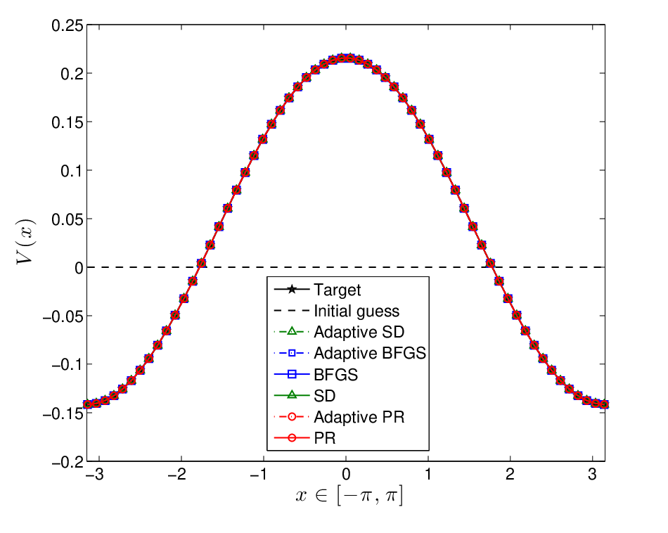
Refer to caption
(a) Potentials
Refer to caption
(b) Bands
Refer to caption
(c) Evolution of ss
Refer to caption
(d) Evolution of pp
Refer to caption
(e) Convergence of the algorithms
Figure 1: Recovery of the cosine potential

In the second test case, we try to recover a more complex potential with pt=8p_{\mathrm{t}}=8 (see Figure 2). In this case, all the algorithms reproduce well the first bands, but fail to recover the potential. Actually, we see how different methods can lead to different local minima for the functional 𝒥\mathcal{J}. This reflects the complex landscape of this function.

Refer to caption
(a) Potentials
Refer to caption
(b) Bands
Refer to caption
(c) Evolution of ss
Refer to caption
(d) Evolution of pp
Refer to caption
(e) Convergence of the algorithms
Figure 2: Recovery of an oscillating potential.

We end this section by reporting results obtained with the different algorithms, and for different target potential Vt∈YptV_{\mathrm{t}}\in Y_{p_{\mathrm{t}}} with pt=1,4,8,12p_{\mathrm{t}}=1,4,8,12 (see Table 1). In this table, NN denotes the number of iterations, sNs_{N} and pNp_{N} are the values of the parameters ss and pp at the last iteration (in particular, for the naive algorithms, we have sN=st=20s_{N}=s_{\mathrm{t}}=20 and pN=ptp_{N}=p_{\mathrm{t}}). Lastly, for each algorithm algo, we define a relative CPU time

τalgo=talgotSD,\tau_{\rm\textbf{algo}}=\dfrac{t_{\rm\textbf{algo}}}{t_{\rm\textbf{SD}}},

where talgot_{\rm\textbf{algo}} is the CPU time consumed by the algorithm algo and tSDt_{\rm\textbf{SD}} is the CPU time consumed by the classical steepest descent. In particular, τSD=1\tau_{\rm\textbf{SD}}=1.

ptp_{\mathrm{t}} - BFGS PR SD
- naive adaptive naive adaptive naive adaptive
11 τ\tau 0.259 1.176 0.929 1.320 1 1.255
NN 8 31 21 154 24 90
sNs_{N} 20 3 20 4 20 3
pNp_{N} 1 3 1 2 1 3
44 τ\tau 0.070 0.009 0.464 0.281 1 0.259
NN 54 1424 1927 7091 8453 19095
sNs_{N} 20 8 20 7 20 5
pNp_{N} 4 5 4 3 4 3
88 τ\tau 0.470 0.151 1.090 0.144 1 0.519
NN 553 1041 1023 1515 7326 26783
sNs_{N} 20 6 20 7 20 6
pNp_{N} 8 4 8 4 8 4
1212 τ\tau 0.007 0.001 0.054 0.004 1 0.044
NN 765 2474 2413 2727 50312 34865
sNs_{N} 20 9 20 9 20 9
pnp_{n} 12 8 12 8 12 8
Table 1: Results for recovery test with different algorithms. Red values are reference values.

We notice that although the adaptive approach requires more iterations to converge, it is usually faster than the naive one. As we already mentioned, this is due to the fact that most of the iterations are performed with small values of pp and ss, and are therefore faster. Moreover, we notice that the adaptive algorithms tend to find an optimised potential which pN≤ptp_{N}\leq p_{\mathrm{t}}, i.e. a less oscillatory potential than the target one.

Ackowledgements

The authors heartily thank Éric Cancès, Julien Vidal, Damiano Lombardi and Antoine Levitt for their great help in this work and for inspiring discussions. The IRDEP institute is acknowledged for funding.

Appendix A A posteriori error estimator for the eigenvalue problem

We present in this appendix the a posteriori error estimator for eigenvalue problems that we use in Section 4.3. More details about this estimator are given in [2].

Let ℋ\mathcal{H} be a finite dimensional space of size NrefN_{\rm ref} and let AA be a self-adjoint operator on ℋ\mathcal{H}. In our case, ℋ\mathcal{H} is some XsrefX_{s_{\rm ref}} for some large sref≫1s_{\rm ref}\gg 1, and A=AqV,srefA=A^{V,s_{\rm ref}}_{q}. The eigenvalues of AA, counting multiplicities are denoted by ε1≤ε2≤⋯≤εNref\varepsilon_{1}\leq\varepsilon_{2}\leq\cdots\leq\varepsilon_{N_{\rm ref}}.

For N≪NrefN\ll N_{\rm ref}, we consider XNX_{N} a finite dimensional subspace of ℋ\mathcal{H}. We denote by ΠXN\Pi_{X_{N}} the orthogonal projection on XNX_{N}, and by AN:=ΠXN​A​ΠXN∗A^{N}:=\Pi_{X_{N}}A\Pi_{X_{N}}^{*}. The eigenvalues of ANA^{N} are denoted by ε1N≤ε2N≤⋯≤εNN\varepsilon_{1}^{N}\leq\varepsilon_{2}^{N}\leq\cdots\leq\varepsilon_{N}^{N}. Let us also denote by (umN)1≤j≤N\left(u_{m}^{N}\right)_{1\leq j\leq N} a corresponding orthogonal basis of XNX^{N}, so that

∀1≤m≤N,AN​umN=εmN​umN.\forall 1\leq m\leq N,\quad A^{N}u_{m}^{N}=\varepsilon_{m}^{N}u_{m}^{N}.

We recall that, from the min-max principle, it holds that εm≤εmN\varepsilon_{m}\leq\varepsilon_{m}^{N}. A certified a posteriori error estimator for the mm-th eigenvalue is a non-negative real number ΔmN∈ℝ+\Delta_{m}^{N}\in\mathbb{R}_{+} such that

εmN−εm≤ΔmN.\varepsilon_{m}^{N}-\varepsilon_{m}\leq\Delta_{m}^{N}.

We also require that the expression of ΔmN\Delta_{m}^{N} only involves the approximated eigenpair εmN\varepsilon_{m}^{N} and umNu_{m}^{N} (and not εm\varepsilon_{m}).

Proposition A.1.

Assume that εm\varepsilon_{m} (resp. εmN\varepsilon_{m}^{N}) is a non-degenerate eigenvalue of AA (resp. ANA^{N}), and that

0<εmN−εm<dist​(εmN,σ⁡(A)∖{εm}).0<\varepsilon_{m}^{N}-\varepsilon_{m}<\mbox{\rm dist}\left(\varepsilon_{m}^{N},\sigma(A)\setminus\left\{\varepsilon_{m}\right\}\right). (A.1)

Let λm<εm\lambda_{m}<\varepsilon_{m}. Then there exists δm>0\delta_{m}>0 such that, for all 0≤δ<δm0\leq\delta<\delta_{m}, we have

εmN−εm≤⟨rmN,(A−cδ)−1​(A−dδ)​(A−cδ)−1​rmN⟩,\varepsilon_{m}^{N}-\varepsilon_{m}\leq\left\langle r_{m}^{N},\left(A-c_{\delta}\right)^{-1}\left(A-d_{\delta}\right)\left(A-c_{\delta}\right)^{-1}r_{m}^{N}\right\rangle, (A.2)

where we set cδ:=εmN+δc_{\delta}:=\varepsilon_{m}^{N}+\delta, dδ:=λm+δd_{\delta}:=\lambda_{m}+\delta, and where rmN:=(A−εmN)​umNr_{m}^{N}:=\left(A-\varepsilon_{m}^{N}\right)u_{m}^{N} is the residual.

Proof.

Assumption (A.1) implies that εmN∉σ⁡(A)\varepsilon_{m}^{N}\notin\sigma\left(A\right), so that (A−εmN)\left(A-\varepsilon_{m}^{N}\right) is invertible. From the fact that ⟨umN,A​umN⟩=εmN\langle u_{m}^{N},Au_{m}^{N}\rangle=\varepsilon_{m}^{N}, and the definition of the residual, it holds that

εmN−εm=⟨rmN,(A−εmN)−1​(A−εm)​(A−εmN)−1​rmN⟩.\varepsilon_{m}^{N}-\varepsilon_{m}=\left\langle r_{m}^{N},\left(A-\varepsilon_{m}^{N}\right)^{-1}\left(A-\varepsilon_{m}\right)\left(A-\varepsilon_{m}^{N}\right)^{-1}r_{m}^{N}\right\rangle. (A.3)

Thus, a sufficient condition for (A.2) to hold is that

(A−cδ)−1​(A−dδ)​(A−cδ)−1≥(A−εmN)−1​(A−εm)​(A−εmN)−1.\left(A-c_{\delta}\right)^{-1}\left(A-d_{\delta}\right)\left(A-c_{\delta}\right)^{-1}\geq\left(A-\varepsilon_{m}^{N}\right)^{-1}\left(A-\varepsilon_{m}\right)\left(A-\varepsilon_{m}^{N}\right)^{-1}.

Thanks to the spectral decomposition of AA, this is the case if and only if,

∀1≤m~≤Nref,εm~−dδ(εm~−cδ)2≥εm~−εm(εm~−εmN)2.\forall 1\leq\widetilde{m}\leq N_{\rm ref},\quad\frac{\varepsilon_{\widetilde{m}}-d_{\delta}}{\left(\varepsilon_{\widetilde{m}}-c_{\delta}\right)^{2}}\geq\frac{\varepsilon_{\widetilde{m}}-\varepsilon_{m}}{\left(\varepsilon_{\widetilde{m}}-\varepsilon_{m}^{N}\right)^{2}}.

Denoting by η:=dist​(εmN,σ⁡(A)∖{εm})−(εmN−εm)\eta:=\mbox{\rm dist}\left(\varepsilon_{m}^{N},\sigma(A)\setminus\left\{\varepsilon_{m}\right\}\right)-\left(\varepsilon_{m}^{N}-\varepsilon_{m}\right), this holds true as soon as δ≤δm:=min⁡(εm−λm,η)\delta\leq\delta_{m}:=\min\left(\varepsilon_{m}-\lambda_{m},\eta\right). The result follows. ∎

In order to use the left-side of (A.2) as an a posteriori estimator, we need to choose λm<εm\lambda_{m}<\varepsilon_{m} and δm>0\delta_{m}>0. For the choice of λm\lambda_{m}, we follow [25], and notice that

εm≥λm:=μ−(Nref−m−1m+1)1/2​σ,\varepsilon_{m}\geq\lambda_{m}:=\mu-\left(\frac{N_{\rm ref}-m-1}{m+1}\right)^{1/2}\sigma,

where we set

μ:=1Nref​Tr​Aandσ2:=1Nref​Tr​A2−μ2.\mu:=\frac{1}{N_{\rm ref}}\mathrm{Tr}\,A\quad\text{and}\quad\sigma^{2}:=\frac{1}{N_{\rm ref}}\mathrm{Tr}\,A^{2}-\mu^{2}.

For the choice of δm\delta_{m}, we chose the simple rule

δm=θ⁡(εmN−κ)with0<θ≪1 and ​κ∈ℝindependent of m.\delta_{m}=\theta\left(\varepsilon_{m}^{N}-\kappa\right)\quad\text{with}\quad 0<\theta\ll 1\quad\text{ and }\kappa\in\mathbb{R}\quad\text{independent of $m$}.

The real number κ\kappa is chosen to be an a priori lower bound of the lowest eigenvalue ε1\varepsilon_{1} of AA. This choice is heuristic in the sense that we cannot guarantee that the assumptions of Proposition A.1 are satisfied. However, the encouraging numerical results we obtain below motivated our choice to use such an estimator (see Section A).

Numerical test

To illustrate the efficiency of our heuristic, we tested it to compute the first bands of the Hill’s operator AVA^{V} with

V⁡(x)=∑k=−33V^k​ek,whereV^0=2andV^−1¯=V^−2¯=V^1=V^2=1+0.5​i.V(x)=\sum\limits_{k=-3}^{3}\hat{V}_{k}e_{k},\quad\text{where}\quad\hat{V}_{0}=2\quad\text{and}\quad\overline{\hat{V}_{-1}}=\overline{\hat{V}_{-2}}=\hat{V}_{1}=\hat{V}_{2}=1+0.5\,i.

The reference operator is A:=AqV,srefA:=A_{q}^{V,s_{\rm ref}} with sref=250s_{\rm ref}=250, and the first three bands are computed on the space XsX^{s} defined in 4.1 with s=6s=6. We plot in Figure 3 the true error εq,mV,s−εq,mV,sref\varepsilon_{q,m}^{V,s}-\varepsilon_{q,m}^{V,s_{\rm ref}} for m=1,2,3m=1,2,3, and the corresponding a posteriori error with κ=0\kappa=0 and different values of θ\theta (namely θ=0.1,0.5,1\theta=0.1,0.5,1). We observe that our estimator is sharp for a large range of θ\theta.

Refer to caption
(a) Potential VV
Refer to caption
(b) m=1m=1
Refer to caption
(c) m=2m=2
Refer to caption
(d) m=3m=3
Figure 3: Numerical validation of the a posteriori error estimator proposed in Appendix A.

References

  • [1] A. Bakhta. Mathematical models and numerical simulation of photovoltaic materials. PhD thesis, Université Paris Est - Ecole des Ponts ParisTech, 2017.
  • [2] A. Bakhta and D. Lombardi. An a posteriori error estimator based on shifts for positive hermitian eigenvalue problems. https://hal.inria.fr/hal-01584180/, 2017.
  • [3] J.F. Bonnans, J.Ch. Gilbert, C. Lemaréchal, and C. Sagastizábal. Numerical Optimization. Springer Verlag, 2003.
  • [4] N.C. Dias, C. Jorge, and J.N. Prata. One-dimensional Schrödinger operators with singular potentials: A Schwartz distributional formulation. J. of Differential Equations, 260(8):6548–6580, 2016.
  • [5] G. Eskin. Inverse spectral problem for the Schrödinger equation with periodic vector potential. Commun. Math. Phys, 125(2):263–300, 1989.
  • [6] J. Eskin, J. Ralston, and E. Trubowiz. On isospectral periodic potential in ℝn\mathbb{R}^{n}. I. Commun. Pure Appl. Maths., 37(5):647–676, 1984.
  • [7] J. Eskin, J. Ralston, and E. Trubowiz. On isospectral periodic potential in ℝn\mathbb{R}^{n}. II. Commun. Pure Appl. Maths., 37(6):715–753, 1984.
  • [8] L.C. Evans. Partial Differential Equations. Graduate studies in mathematics. American Mathematical Society, 1998.
  • [9] G. Freiling and V. Yurko. Inverse Sturm-Liouville problems and their applications. Nova Science Publishers, 2001.
  • [10] F. Gesztesy and M. Zinchenko. On spectral theory for Schrödinger operators with strongly singular potentials. Math. Nachr., 279(9-10):1041–1082, 2006.
  • [11] R.O. Hryniv and Y.V. Mykytyuk. 1-D Schrödinger operators with periodic singular potentials. Methods Funct. Anal. Topology, 7(4):31–42, 2001.
  • [12] R.O. Hryniv and Y.V. Mykytyuk. Inverse spectral problems for Sturm-Liouville operators with singular potentials. Inverse Problems, 19(3):665, 2003.
  • [13] R.O. Hryniv and Y.V. Mykytyuk. Inverse spectral problems for Sturm-Liouville operators with singular potentials. III. Reconstruction by three spectra. J. Math. Anal. Appl., 284(2):626–646, 2003.
  • [14] R.O. Hryniv and Y.V. Mykytyuk. Half-inverse spectral problems for Sturm-Liouville operators with singular potentials. Inverse Problems, 20(5):1423, 2004.
  • [15] R.O. Hryniv and Y.V. Mykytyuk. Inverse spectral problems for Sturm-Liouville operators with singular potentials. II. Reconstruction by two spectra. North-Holland Mathematics Studies, 197:97–114, 2004.
  • [16] R.O. Hryniv and Y.V. Mykytyuk. Inverse spectral problems for Sturm-Liouville operators with singular potentials. IV. Potentials in the Sobolev space scale. Proceedings of the Edinburgh Mathematical Society, 49(2):309–329, 2006.
  • [17] T. Kato. Schrödinger operators with singular potentials. Israel Journal of Mathematics, 13(1):135–148, 1972.
  • [18] P. Kuchment. An overview of periodic elliptic operators. Bull. Amer. Math. Soc., 53(3):343–414, 2016.
  • [19] E.H. Lieb and M. Loss. Analysis, volume 14 of Graduate studies in mathematics. 2001.
  • [20] V. Mikhaelets and V. Molyboga. One-dimensional Schrödinger operators with singular periodic potentials. Methods Funct. Anal. Topology, 14(2):184–200, 2008.
  • [21] J. Pöschel and E. Trubowiz. Inverse spectral theory. Pure and applied mathematics. Academic Press, 1987.
  • [22] M. Reed and B. Simon. Methods of modern mathematical physics. IV: Analysis of operators. Elsevier, 1978.
  • [23] N.S. Trudinger. On Harnack type inequalities and their application to quasilinear elliptic equations. Commun. Appl. Math., 20(4):721–747, 1967.
  • [24] O. Veliev. Multidimensional periodic Schrödinger operator. Perturbation theory and applications. Academic Press, 2015.
  • [25] H. Wolkowicz and G.P.H. Styan. Bounds on eigenvalues using traces. Linear Algebra Appl., 29:471–506, 1980.