The Devil is in the Details: Spectrum and Eigenvalue Distribution of the Discrete Preisach Memory Model

Hysteresis modeling has been an active area of research for decades with a wide range of physics-based, phenomenological and mathematical models ([44, 11, 34, 28, 45, 33]). In 1935, F. Preisach proposed his well-known input-state-output model for ferromagnetic hysteresis [35]. The evolution of states in this model has been later shown to be universal for many important models of hysteresis with scalar-valued inputs and outputs [10, 29] or, more precisely, for all the models which respect Madelung’s memory update rules (also known as hysteresis with return point memory or the wiping out property [40]).

In its discrete form, the Preisach model describes the state of magnetic domains (moments) in a magnetic medium as illustrated in Figure 1, where the coordinates $\alpha,\beta$ are parameters (called thresholds) associated with the magnetic domains. Here, the center of each dark gray unit box represents a magnetic moment pointing “up” and the center of each light gray unit box corresponds to a magnetic moment pointing “down”. The state of the system is represented by the staircase line $L$ separating the dark and light gray areas. This line of length $N$ consists of horizontal and vertical unit segments and it connects the point $(0,N)$ with a point $(i,i)$ on the diagonal $\alpha=\beta$. Starting at the upper left end $(0,N)$, the line $L$ can be encoded by a unique $N$-tuple of $0^{\prime}$s and $1^{\prime}$s, corresponding to vertical unit segments and horizontal unit segments, respectively.

The input $i\in\{0,1,\ldots,N\}$ of the discrete Preisach model (which provides the coordinates $(i,i)$ of the lower right end of the staircase line $L$) describes the influence of the external field. The input $i$ can change by $\pm 1$ at each time step, after which the lower right end of $L$ moves accordingly. Further, when $i$ is increased, all the horizontal segments are passed from left to right, and when $i$ is decreased, all the vertical segments are passed in the downward direction. In other words, the rules of updating the state require that the smallest possible number of unit boxes change their color, see Figure 1.

A last-in-first-out (LIFO) model can also be associated with these rules. Consider a one dimensional storage with $N$ spaces. A space is labeled by $0$ if empty and by $1$ if occupied by a box (element). A stored element takes exactly one space, thus the state of the storage is an $N$-tuple of $0^{\prime}$s and $1^{\prime}$s. Elements can be added to, or removed from, the storage through the entrance/exit at the right end. Suppose the following rules apply: when an element is added to the stock, it is placed to the free space nearest the entrance; similarly, the element nearest the entrance is removed when the “removal” operation is applied. The order in which elements come off the storage according to this protocol can be characterized as last-in-first-out because we always remove the most recently added element.¹¹ 1 Note that this protocol is different from a similar protocol known as stack data type in computer science. The transition induced by an increase of the input corresponds to adding an element to the storage, while the transition induced by a decrease of the input corresponds to removing an element from the storage.

In the above models, variations of the input induce transitions between the states, which are equivalent to transitions described by an underlying graph $\Gamma$. The graph $\Gamma$ is self-similar with interesting properties. The goal of this paper is to describe and formally prove some of these properties (for example, we show that the adjacency matrix of $\Gamma$ has a self-similar eigenvalue distribution), offering an example of analytical treatment of a self-similar graph to the wider scientific community. Self-similar matrices and graphs appear in distinct areas. Kostadinov [27] expresses the free energy of a one-dimensional Ising model with random couplings in terms of the maximal eigenvalue of a self-similar matrix. He also relates the calculation for the spectra of molecular type of systems in the tight binding approximation to the eigenvalues and eigenvectors of self-similar Hermitian matrices. Stosic et al. [42] find the analytical expression for the residual entropy of the two-dimensional Ising model with nearest-neighbor antiferromagnetic coupling in terms of the fractal Fibonacci matrix. Katsanos and Evangelou [24] study the level-spacing distribution of a fractal Fibonacci matrix to address questions related to Anderson localization and quantum chaos. Hsu et al. introduced Fibonacci cubes as a new class of self-similar graphs [23]. Ferrand [17] considers a self-similar matrix related to the Thue-Morse sequence.

Many real networks can also be categorized as self-similar [41]. Generating realistic networks is a subject of intense study. Barriere et al. [5] investigate the generalized hierarchical product of graphs. Leskovec et al. [31] propose a network generation model based on the Kronecker product. Komjáthy and Simon [25] introduce deterministic scale-free networks derived from a graph directed self-similar fractal. Many books have been written recently on complex networks and graphs, see, for example [chung2006complex].

The eigenvalues of the adjacency matrix are related to important properties of the graph (for a good introduction to spectral graph theory, see, for example, [12]). The largest eigenvalue of the adjacency matrix of a graph plays a key role in several respects, including in synchronization of oscillators, percolation on directed networks and linear stability of equilibria of coupled systems.

The paper is structured as follows. In Section 2 we introduce the necessary notation and define the graphs studied. Section 3 describes the properties of the adjacency matrix $A_{n}$. In Section 4 we look at the eigenvalue distribution of the (non-symmetric) adjacency matrix. Section 5 provides explicit description of the eigenvectors of $A_{n}$. Section 6 concludes our work.

Consider the set $\{0,1\}^{N}$ of all $N$-tuples $\mathbf{x}=(x_{0},\ldots,x_{N-1})$ with $x_{i}\in\{0,1\}$ (this is the Hamming space of all $2^{N}$ binary strings of length $N$). Let us associate a vertex of a directed graph $\Gamma$ with every $N$-tuple. Define the set of directed edges of $\Gamma$ according to the rules

1. $(H_{1})$

   The vertex $\mathbf{0}=(0,0,\ldots 0,0,0)$ only has one direct successor $(0,0,\ldots 0,0,1)$;

2. $(H_{2})$

   The vertex $\mathbf{1}=(1,1,\ldots 1,1,1)$ only has one direct successor $(1,1,\ldots 1,1,0)$;

3. $(H_{3})$

   Every other vertex $\mathbf{x}$ has two direct successors $\mathbf{y}$ and $\mathbf{z}$ defined as follows:

   $$x_{i}=0;\quad x_{i+1}=\cdots=x_{N-1}=1\quad\Rightarrow\quad y_{i}=1,\quad y_{k}=x_{k}\ \mathrm{for}\ k\neq i;$$

   $$x_{j}=1;\quad x_{j+1}=\cdots=x_{N-1}=0\quad\Rightarrow\quad z_{j}=0,\quad z_{k}=x_{k}\ \mathrm{for}\ k\neq j.$$

In other words, $N$-tuple $\mathbf{y}$ is obtained by replacing the rightmost $0$ in the $N$-tuple $\mathbf{x}=(x_{0},\ldots,x_{N-1})$ with $1$ and $\mathbf{z}$ is obtained by replacing the rightmost $1$ in the $N$-tuple $\mathbf{x}=(x_{0},\ldots,x_{N-1})$ with $0$. For example, the vertex $(1,0,1,0,1)$ is connected to the vertices $(1,0,1,0,0)$ and $(1,0,1,1,1)$.

The adjacency matrix $A_{N}$ (of order $2^{N}$) of graph $\Gamma$ can recursively be defined by the relations

where $J_{k}$ and $J_{k}^{\prime}$ are diagonal matrices of order $2^{k}$ defined by

For example,

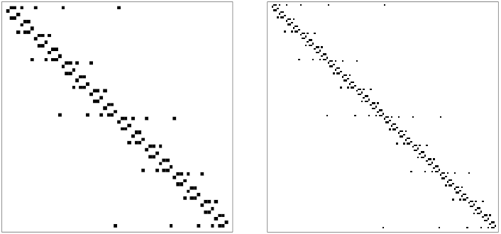
Due to its recursive definition, $A_{n}$ is a block-hierarchical matrix, i.e. a matrix where hierarchically nested growing blocks are placed along the diagonal, where each (sub-)block is again a block-hierarchical matrix itself [19]. Figure 2 illustrates the graphs corresponding to $A_{1},A_{2},$ $A_{3}$, and $A_{9}$, while Figure 3 demonstrates the connection structure of the adjacency matrices $A_{6}$ and $A_{7}$ (the 1’s are shown as black dots).

Let us denote by $\Gamma^{\prime}$ the graph obtained from $\Gamma$ by adding self-loops at vertices $\mathbf{0}$ and $\mathbf{1}$. This is achieved by replacing rules $(H_{1})$, $(H_{2})$ with

• $(H_{1}^{\prime})$

  The vertex $\mathbf{0}=(0,0,\ldots 0,0,0)$ has two direct successors, $(0,0,\ldots 0,0,1)$ and $\mathbf{0}$;

• $(H_{2}^{\prime})$

  The vertex $\mathbf{1}=(1,1,\ldots 1,1,1)$ has two direct successors, $(1,1,\ldots 1,1,0)$ and $\mathbf{1}$.

Spectral graph theory (see, for example, [12]) relates the eigenvalues of the adjacency matrix to other properties of the graph. We are thus interested in the spectrum

and eigenvalue distribution

of the matrix $\frac{1}{2}A_{N}$ and the $N\rightarrow\infty$ limit of these objects. Here $\#\Omega$ denotes the cardinality of the set $\Omega$. Figure 4 shows the Devil’s staircase eigenvalue distribution for $A_{12}$.

Xiuqing and Youyan [46] and Fu et al. [18] studied one-dimensional Fibonacci-class quasilattices and showed that for these types of lattices the energy spectrum exhibits a staircase behavior. He et al. [20, 21] studied a family of trees (the interior nodes have degree $k$ and the boundary nodes have degree 1) and found that the eigenvalue distributions approach a piecewise constant “Cantor function.”Spectral properties of structured matrices have been extensively studied. Banded Toeplitz matrices are the topic of the book by Bottcher and Grudsky [9]. A classical result of Schmidt-Spitzer [38] and Hirschman [22] is that the eigenvalues accumulate on a special curve in the complex plane and the normalized eigenvalue counting measure converges weakly to a measure on this curve as $N\rightarrow\infty$. Duits and Kuijlaars [16] study the limiting eigenvalue distribution of $N\times N$ banded Toeplitz matrices as $N\rightarrow\infty$, and characterize the limiting measure in terms of an equilibrium problem. Even though the spectrum of the limiting operator need not mimic that of the finite-dimensional operator, pseudospectra and numerical ranges behave nicely [9]. The pseudospectra of $A_{5}$ and $A_{8}$ are shown in Figure 5.

Interestingly, Devil’s staircases have been associated with the one-dimensional Ising model with antiferromagnetic interactions [3]. Exact eigenvalues and eigenvectors of different one-dimensional quantum many-body models starting with the Hamiltonian of the antiferromagnetic Heisenberg model have been obtained using the Bethe ansatz [6, 8].

In this section, we consider the distribution function (empirical spectral distribution, density of states)

of the eigenvalues of the matrix $\frac{1}{2}A_{N}$ and its $N\rightarrow\infty$ limit (limiting spectral distribution). By definition, $F_{N}$ is an increasing piecewise constant left-continuous function with a finite number of jumps. Since the spectrum of the matrix $\frac{1}{2}{A_{N}}$ belongs to the interval $(-1,1)$, it also follows that $F_{N}(x)=0$ for $x\leq-1$ and $F_{N}(x)=1$ for $x\geq 1$.

The following Devil’s staircase function [4, 7, 14] has received substantial attention in the literature:

where $\lfloor\cdot\rfloor$ denotes the floor (integer value) function. We consider the extension of $f$ to the whole axis according to the formulas

This extension is an increasing right continuous function. At every rational point $x_{i}=r/q\in(0,1)$, where $r,q>0$ are coprime integers, the function $f$ has a jump

and $f$ is continuous at every irrational point. As a matter of fact, equation (18) is equivalent to

Further, the total sum of all the jumps of $f$ satisfies

where $\varphi$ is Euler’s totient function. Hence, this sum equals the total variation $f(1)-f(0)=1$ of $f$, and therefore $f$ is a jump function [2], i.e.

with the sum over all the rational points $x_{i}\in(0,x)$.

This theorem is proved in the next section. From formulas (7), (8), it follows that the distribution function of the spectrum of the matrix $\frac{1}{2}A_{N}^{\prime}$ converges to the same limit as $N\rightarrow\infty$. It should be noted that the algebraic and geometric multiplicities of eigenvalues are different.

Eigenvectors and eigenspaces of graphs are also important [13], [43]. For example they are used to count walks in a graph and to relate the symmetry of a graph to its spectrum. The principal eigenvector of the adjacency matrix provides vertex centrality information, while the second eigenvector can be used to partition the graph into clusters. The eigenvectors are related to the graph’s automorphic structure.

Let us now study the eigenvectors of $\frac{1}{2}A_{N}$. In order to do this, let us first make the notation for vertices more efficient. In the following, let us identify a vertex with the corresponding string of $0$s and $1$s, for example,

Strings are concatenated by simply writing one after the other. We will use the notation $1^{j}$ to denote a string with $j$ ones and $0^{j}$ for a string with $j$ zeros. For example, $\left(11001\right)=\left(1^{2}0^{2}1\right)$. For consistency, it is convenient to agree that $0^{0}$ and $1^{0}$ is an empty string. Also for convenience, let us introduce the symmetry operation $S$, which replaces every $0$ in a string with a $1$ and vice versa, for example, $S\left(11001\right)=\left(00110\right)$. Obviously, $S$ is an involution.

An arbitrary binary string of length $j$ will be denoted by $q^{j}$, and the set of all strings of length $j$ will be denoted by $W_{j}$. In particular, the matrix $\frac{1}{2}A_{N}$ acts in the $2^{N}$-dimensional vector space $V$ spanned by the vertices $(q^{N})\in W_{N}$.

Consider an expansion of an eigenvector $v\in V$ of $\frac{1}{2}A_{N}$ along the basis $W_{N}$:

According to Theorem 1, $\lambda$ is a root of a Chebyshev polynomial $U_{\ell}$ with $\ell=1,\ldots,N-1$ or $\ell=N+1$. We would like to determine the $2^{N}$ components $c_{(q^{N})}$ of an eigenvector $v$ (up to a scaling factor).

Note that the identity $U_{k}^{2}-1=U_{k-1}U_{k+1}$ implies $U_{\ell}^{2}(\lambda)=1$ under the conditions of Theorem 4 because $U_{\ell+1}(\lambda)=0$. Since $(q^{N-\ell-2})\in W_{N-\ell-2}$ is arbitrary, the geometric multiplicity of such an eigenvalue is $2^{N-\ell-2}$.

As an example, if $\lambda=1/\sqrt{2}$, then $U_{3}(\lambda)=0$ and $U_{1}(\lambda)=\sqrt{2},U_{2}(\lambda)=1$. According to Theorem 4, $2^{N-4}$ linearly independent eigenvectors corresponding to the eigenvalue $\lambda=1/\sqrt{2}$ can be labeled by the strings $(q^{N-4})\in W_{N-4}$, and the components of an eigenvector are defined by

References

- [1] A. Amann, M. Brokate, S. McCarthy, D. Rachinskii, and G. Temnov. Characterization of memory states of the Preisach operator with stochastic inputs. Physica B: Condensed Matter, 407(9):1404–1411, 2012.
- [2] L. Ambrosio, N. Fusco, and D. Pallara. Functions of bounded variation and free discontinuity problems. Oxford University Press, 2000.
- [3] S. Aubry. Exact models with a complete Devil’s staircase. J. Phys. C: Solid State Phys., 16:2497–2508, 1983.
- [4] D. H. Bailey and R. E. Crandall. Random generators and normal numbers. Exper. Math., 11:527–546, 2002.
- [5] L. Barrière, C. Dalfó, M. A. Fiol, and M. Mitjana. The generalized hierarchical product of graphs. Discrete Mathematics, 309(12):3871–3881, 2009.
- [6] R. J. Baxter. Exactly solved models in statistical mechanics. Academic Press, 1982.
- [7] P. E. Böhmer. über die transcendenz gewisser dyadischer brüche. Math. Ann., 96:367–377, 1926.
- [8] C. J. Bolech and N. Andrei. Solution of the two-channel anderson impurity model: Implications for the heavy fermion UBe13. Phys. Rev. Lett., 88:237206, 2002.
- [9] A. Böttcher and S. M. Grudsky. Spectral properties of banded Toeplitz matrices. SIAM, 2005.
- [10] M. Brokate and J. Sprekels. Hysteresis and phase transitions, volume 121. Springer Science & Business Media, 2012.
- [11] M. Brokate and A. Visintin. Properties of the Preisach model for hysteresis. J. Reine Angew. Math., 402:1–40, 1989.
- [12] F. R. Chung. Spectral graph theory, volume 92. American Mathematical Soc., 1997.
- [13] D. M. Cvetković, P. Rowlinson, and S. Simic. Eigenspaces of graphs, volume 66. Cambridge University Press, 1997.
- [14] J. L. Davison. A series and its associated continued fraction. Proc. Amer. Math. Soc., 63:29–32, 1977.
- [15] M. Dimian and P. Andrei. Noise-Driven Phenomena in Hysteretic Systems. Springer, 2013.
- [16] M. Duits and A. B. Kuijlaars. An equilibrium problem for the limiting eigenvalue distribution of banded Toeplitz matrices. SIAM J. Matrix Analysis and Applications, 30(1):173–196, 2008.
- [17] E. Ferrand. An analogue of the Thue-Morse sequence. The Electronic Journal of Combinatorics, 14(1):R30, 2007.
- [18] X. Fu, Y. Liu, P. Zhou, and W. Sritrakool. Perfect self-similarity of energy spectra and gap-labeling properties in one-dimensional Fibonacci-class quasilattices. Physical Review B, 55(5):2882, 1997.
- [19] B. Gutkin and V. A. Osipov. Spectral problem of block-rectangular hierarchical matrices. Journal of Statistical Physics, 143(1):72–87, 2011.
- [20] L. He, X. Liu, and G. Strang. Laplacian eigenvalues of growing trees. In Conf. on Math. Theory of Networks and Systems, 2000.
- [21] L. He, X. Liu, and G. Strang. Trees with Cantor eigenvalue distribution. Studies in Applied Mathematics, 110(2):123–138, 2003.
- [22] I. Hirschman et al. The spectra of certain Toeplitz matrices. Illinois Journal of Mathematics, 11(1):145–159, 1967.
- [23] W.-J. Hsu and J.-S. Liu. Fibonacci cubes - a class of self-similar graphs. In Fibonacci Quart. Citeseer, 1993.
- [24] D. Katsanos and S. Evangelou. Level-spacing distribution of a fractal matrix. Physics Letters A, 289(4):183–187, 2001.
- [25] J. Komjáthy and K. Simon. Generating hierarchial scale-free graphs from fractals. Chaos, Solitons & Fractals, 44(8):651–666, 2011.
- [26] C. E. Korman and I. D. Mayergoyz. Preisach model driven by stochastic inputs as a model for aftereffect. IEEE Transactions on Magnetics, 32(5), 1996.
- [27] I. Kostadinov. Fractal Hamiltonians in condensed matter physics. Physica Scripta, 36(3):516, 1987.
- [28] M. A. Krasnosel’skii and A. V. Pokrovskii. Systems with hysteresis. Springer Science & Business Media, 2012.
- [29] P. Krejčí. Hysteresis, convexity and dissipation in hyperbolic equations. Gattotoscho, 1996.
- [30] P. Krejčı, J. P. O’Kane, A. Pokrovskii, and D. Rachinskii. Properties of solutions to a class of differential models incorporating preisach hysteresis operator. Physica D: Nonlinear Phenomena, 241(22):2010–2028, 2012.
- [31] J. Leskovec, D. Chakrabarti, J. Kleinberg, C. Faloutsos, and Z. Ghahramani. Kronecker graphs: An approach to modeling networks. Journal of Machine Learning Research, 11(Feb):985–1042, 2010.
- [32] J. C. Mason and D. C. Handscomb. Chebyshev polynomials. CRC Press, 2002.
- [33] I. Mayergoyz and G. Bertotti, editors. The science of hysteresis. Academic Press, 2005.
- [34] I. D. Mayergoyz. Mathematical models of hysteresis and their applications. Academic Press, 2003.
- [35] F. Preisach. Über die magnetische nachwirkung. Zeitschrift für Physik, 94(5-6):277–302, 1935.
- [36] D. Rachinskii and M. Ruderman. Convergence of direct recursive algorithm for identification of preisach hysteresis model with stochastic input. SIAM J. Appl. Math., 76(4):1270–1295, 2016.
- [37] G. Radons. Spectral properties of the preisach hysteresis model with random input. i. general results. Physical Review E, 77(6):061133, 2008.
- [38] P. Schmidt and F. Spitzer. The Toeplitz matrices of an arbitrary Laurent polynomial. Math. Scand, 8(15-38):11J, 1960.
- [39] S. Schubert and G. Radons. Preisach models of hysteresis driven by markovian input processes. Physical Review E, 96(2):022117, 2017.
- [40] J. P. Sethna, K. Dahmen, S. Kartha, J. A. Krumhansl, B. W. Roberts, and J. D. Shore. Hysteresis and hierarchies: Dynamics of disorder-driven first-order phase transformations. Phys. Rev. Lett., 70:3347–3350, 1993.
- [41] C. Song, S. Havlin, and H. A. Makse. Self-similarity of complex networks. Nature, 433(7024):392–395, 2005.
- [42] B. D. Stosic, T. Stosic, I. P. Fittipaldi, and J. Veerman. Residual entropy of the square Ising antiferromagnet in the maximum critical field: the Fibonacci matrix. Journal of Physics A: Mathematical and General, 30(10):L331, 1997.
- [43] P. Van Mieghem. Graph spectra for complex networks. Cambridge University Press, 2010.
- [44] A. Visintin. On the Preisach model for hysteresis. Nonlinear Analysis: Theory, Methods & Applications, 8(9):977–996, 1984.
- [45] A. Visintin. Differential models of hysteresis, volume 111. Springer Science & Business Media, 2013.
- [46] H. Xiuqing and L. Youyan. Spectral structure and gap-labeling properties for a new class of one-dimensional quasilattices. Chinese Physics Letters, 9(11):609, 1992.