跳到论文正文
W Papers独立论文阅读器 arXiv:1709.06910 论文正文 计算阅读时间 · 0%
引用这篇论文根据当前论文元数据生成,正式投稿前建议核对。


License: arXiv.org perpetual non-exclusive license
arXiv:1709.06910v1 [cs.GT] 20 Sep 2017

Linear Quadratic Games with Costly Measurements

This article is an unabridged version of [1].
Dipankar Maity Note: The authors are with the Department of Electrical and Computer Engineering and The Institute for Systems Research, University of Maryland, College Park, MD, USA. Email: dmaity@umd.edu, baras@umd.edu. Research partially supported by DARPA grant W911NF-14-1-0384 through ARO, NSF grant CNS-1544787, and DARPA STTR contract with Boston Engineering Corporation.    Achilleas Anastasopoulos Note:  The author is with the Department of Electrical Engineering and Computer Science, University of Michigan, Ann Arbor, MI, USA. Email: anastas@umich.edu    John S. Baras†
Abstract

In this work we consider a stochastic linear quadratic two-player game. The state measurements are observed through a switched noiseless communication link. Each player incurs a finite cost every time the link is established to get measurements. Along with the usual control action, each player is equipped with a switching action to control the communication link. The measurements help to improve the estimate and hence reduce the quadratic cost but at the same time the cost is increased due to switching. We study the subgame perfect equilibrium control and switching strategies for the players. We show that the problem can be solved in a two-step process by solving two dynamic programming problems. The first step corresponds to solving a dynamic programming for the control strategy and the second step solves another dynamic programming for the switching strategy.

1 Introduction

Linear quadratic (LQ) stochastic games have attracted a great deal of attention in the control and related community due to its wide applicability in stochastic control, minimax control, multi-agent systems and economics [2], [3], [4], [5], [6], [7], [8]. There is a well established notion of (Nash) equilibrium (NE) strategies for static games, and in dynamic games there are refinements of NE known as subgame perfect equilibria (SPE). Closed form solutions for these NE (or SPE) may generally not exist or hard to compute if one such exists. Among the various classes of dynamic games, LQ games exhibit a closed form expression for SPE, and it is characterized by some Riccati equations. Necessary and sufficient conditions for the NE strategies of LQ games have been studied in [4], [9],[6]. Contrary to the prior belief, [10] shows existence of nonlinear control strategies for LQ games.

Amongst the vast majority of the prior works, the underlying assumption is the availability of free observations. Dynamic games are studied with either open-loop strategy (i.e. only measurement is the initial state) or feedback strategies where the observation is available freely at any time. Challenges emerge when the measurements are on demand, but costly. This adds an extra layer of decision making, for the players, because now they have to both, control the system and ask for measurements.

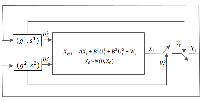
In this work, we consider a class of two-player linear quadratic stochastic games of finite horizon. The game dynamics are partially observable. Contrary to the existing literature, the observations are not freely available. Each observation requires a finite cost for establishing a link for communication. The link through which the observations are communicated to the players (their controllers) is noiseless but operated by two switches (Figure 1), one for each player. The link is established only when both the players are willing for it, and they both get the actual state measurement at that time. Consequently, there is an apparent trade off between cost of obtaining state measurement and the estimation quality.
Refer to caption
Figure 1: Schematic of the system. Each player has to select their controller strategy gig^{i} and switching strategy sis^{i}. All the links are noiseless and delay-free.

In this game, the players can make a precise estimate of the state if they establish the link at every time instance. However, since the link establishment is costly, they can compromise the estimation accuracy in exchange of the cost for accessing the measurement. Therefore, the problem is to optimally decide when to establish the link and how to use the acquired measurement in order to minimize their individual cost. Since, in general, the players will have different preferences over the time instances when they want to acquire the measurement, they have to come to an agreement when to actually establish the link.

The closest work on the similar game framework has been studied in [11] where the authors studied zero-sum stochastic differential LQ games. However, the selection for switching times were performed in an collaborative way rather than being the outcome of a strategic interaction. The major digression of this work from [11] is that we consider an explicit game for the switching strategy as well. We express the switch as a Boolean control action and seek for SPE for both control and switching strategies.

Our contributions are as follows:
(a) We study the SPE of this dynamic game and show that they can be found through a two-step process. Specifically, in the first step we fix the switching strategy and study the SPE for control strategies. The study shows that the control strategy is linear in estimated state, where the gain is characterized with two backward Riccati equations which can be computed offline. Moreover, the Riccati equations do not depend on the switching strategy.
(b) Regarding the equilibrium switching strategy, we provide a backward recursive algorithm to find all SPE where value functions need only be computed over a finite and quadratically-sized (in the duration of the game) set.
(c) Regarding the equilibrium switching strategy, we show that there are many equilibria among which there is one that is strictly preferable by both users and has a Markovian structure. It is found in our study that a strictly preferable switching strategy for a player not only depends on their own cost-to-go, but also depends on the cost-to-go for the opponent.

The remaining of the paper is organized as follows: The problem formulation is provided in Section 2, Section 3 contains the results on the SPE of the control strategy, SPE for the switching strategy and its offline computation are analyzed in Section 4. Finally we conclude our work in Section 6.

2 Problem Formulation

In the discrete time Gauss-Markov setting, we consider the following linear dynamics of the state XtX_{t}:

Xt+1=A​Xt+B1​Ut1+B2​Ut2+WtX_{t+1}=AX_{t}+B^{1}U^{1}_{t}+B^{2}U^{2}_{t}+W_{t} (1)

where Xt∈𝒳=ℝnX_{t}\in\mathcal{X}=\mathbb{R}^{n}, and Uti∈𝒰i=ℝmU^{i}_{t}\in\mathcal{U}^{i}=\mathbb{R}^{m} denotes the action of player ii. Wt∈ℝnW_{t}\in\mathbb{R}^{n} is a Gaussian noise with 𝔼⁡[Wt]=0\mathbb{E}[W_{t}]=0 and 𝔼[WtWs′]=Sδt−s\mathbb{E}[W_{t}W_{s}^{{}^{\prime}}]=S\delta_{t-s} (δt\delta_{t} is the Kronecker delta.), and X0∼𝒩⁡(0,Σ0)X_{0}\sim\mathcal{N}(0,\Sigma_{0}).

There are two additional actions (switching actions) Vt1∈{0,1}V^{1}_{t}\in\{0,1\} and Vt2∈{0,1}V^{2}_{t}\in\{0,1\}. These switching actions control a switch (switch closes if both are equal to 1) and the observation available to both users is Yt∈𝒳∪{e}Y_{t}\in\mathcal{X}\cup\{e\} with

Yt={Xt,V1t=V2t=1e,else,\displaystyle Y_{t}=\left\{\begin{array}[]{ll}X_{t}&,V^{1}_{t}=V^{2}_{t}=1\\ e&,\text{else},\end{array}\right.

where “ee” denotes an erasure. The evolution of random variables in period tt is assumed to be ...Xt→(Vt1,Vt2)→Yt→(Ut1,Ut2)…...X_{t}\rightarrow(V^{1}_{t},V^{2}_{t})\rightarrow Y_{t}\rightarrow(U^{1}_{t},U^{2}_{t})...

The information available at time tt to player ii before she takes the switching action VtiV^{i}_{t} is

It=(Yt−1,U1,t−1,U2,t−1,V1,t−1,V2,t−1),\displaystyle I_{t}=(Y^{t-1},U^{1,t-1},U^{2,t-1},V^{1,t-1},V^{2,t-1}), (4)

and the information available at time tt to player ii before she takes the control action UtiU^{i}_{t} is

I¯t=(It,Vt1,Vt2,Yt).\displaystyle\bar{I}_{t}=(I_{t},V^{1}_{t},V^{2}_{t},Y_{t}). (5)

As a result, the actions have the functional form

Vti\displaystyle V^{i}_{t} =sti(It),i=1,2,\displaystyle=s^{i}_{t}(I_{t}),\qquad i=1,2, (6a)
Uti\displaystyle U^{i}_{t} =gti(I¯t),i=1,2,\displaystyle=g^{i}_{t}(\bar{I}_{t}),\qquad i=1,2, (6b)

where by gi=(gti)t=0T−1g^{i}=(g^{i}_{t})_{t=0}^{T-1}, si=(sti)t=0T−1s^{i}=(s^{i}_{t})_{t=0}^{T-1}, we denote the control and switching strategies of player ii. ∀t∈{0,⋯,T−1}\forall t\in\{0,\cdots,T-1\}, let us denote an ItI_{t} measurable random variable Δt=Vt1⋅Vt2\Delta_{t}=V^{1}_{t}\cdot V^{2}_{t}.

The individual cost that each player needs to minimize is quadratic in state and action, and it also depends on the switching actions Vt1V^{1}_{t} and Vt2V^{2}_{t}. We consider a game for a finite duration ({0,⋯,T}\{0,\cdots,T\}) and the per-stage costs are explicitly written as:

Cti​(xt,ut1,ut2,vt1,vt2)=\displaystyle{C}^{i}_{t}(x_{t},u^{1}_{t},u^{2}_{t},v^{1}_{t},v^{2}_{t})= ‖xt‖Qi2+‖uti‖Qi​i2+‖utj‖Qi​j2+λi​(vti⋅vtj)\displaystyle\|x_{t}\|^{2}_{Q^{i}}+\|u^{i}_{t}\|^{2}_{Q^{ii}}+\|u^{j}_{t}\|^{2}_{Q^{ij}}+\lambda_{i}(v^{i}_{t}\cdot v^{j}_{t}) (7)

for all t∈{0,⋯,T−1}t\in\{0,\cdots,T-1\} and

CTi​(xt,ut1,ut2,vt1,vt2)=‖xT‖Qi2.{C}_{T}^{i}(x_{t},u^{1}_{t},u^{2}_{t},v^{1}_{t},v^{2}_{t})=\|x_{T}\|^{2}_{Q^{i}}. (8)

The quantity λi>0\lambda_{i}>0 is the cost paid by player ii when both the players attempt to close the switch and they observe the state information XtX_{t}. Therefore the average cost over the time horizon {0,⋯,T}\{0,\cdots,T\} is represented as,

Ji​(σ1,σ2)=∑t=0T𝔼⁡[Cti​(Xt,Ut1,Ut2,Vt1,Vt2)]J^{i}(\sigma^{1},\sigma^{2})=\sum_{t=0}^{T}\mathbb{E}[{C}_{t}^{i}(X_{t},U^{1}_{t},U^{2}_{t},V^{1}_{t},V^{2}_{t})] (9)

where σi=(gi,si)\sigma^{i}=(g^{i},s^{i}) denotes the strategy of the player ii that corresponds to control strategy gig^{i} and switching strategy sis^{i}.

The objective of player ii is:

minσi⁡Ji​(σ1,σ2)=minsi⁡{mingi⁡Ji​(σ1,σ2)}\min_{\sigma^{i}}J^{i}(\sigma^{1},\sigma^{2})=\min_{s^{i}}\{\min_{g^{i}}J^{i}(\sigma^{1},\sigma^{2})\} (10)

3 Subgame Perfect Control Strategy

For dynamic games with complete information the appropriate equilibrium concept is a refinement of Nash equilibrium (NE) called the subgame perfect equilibrium (SPE). A strategy profile (σ1,σ2)(\sigma^{1},\sigma^{2}) is a SPE if the restriction of (σ1,σ2)(\sigma^{1},\sigma^{2}) to any proper subgame of the original game constitutes a NE [12, pp. 94].

We seek to characterize the SPE (σ1∗,σ2∗)(\sigma^{1*},\sigma^{2*}) for this switched LQG game. Moreover, we will show that among the multiple SPE, there exists one that simultaneously minimizes the cost for both users among all SPE and thus it will be the preferable SPE solution of this game. In this section, we study the SPE control strategy for both the players.

Theorem 3.1

For any switching profile (s1,s2)(s^{1},s^{2}) of the players, the SPE control strategy gi∗g^{i*} has the following structure:

Uti\displaystyle U^{i}_{t} =gti∗(I¯t)=−LtiX^t,\displaystyle=g^{i*}_{t}(\bar{I}_{t})=-L^{i}_{t}\hat{X}_{t}, (11)

where

X^t={A​X^t−1+B1​Ut−11+B2​Ut−12,Vt1⋅Vt2=0Xt,Vt1⋅Vt2=1.\displaystyle\hat{X}_{t}=\left\{\begin{array}[]{ll}A\hat{X}_{t-1}+B^{1}U^{1}_{t-1}+B^{2}U^{2}_{t-1},&V^{1}_{t}\cdot V^{2}_{t}=0\\ X_{t},&V^{1}_{t}\cdot V^{2}_{t}=1.\end{array}\right.

Furthermore, the cost-to-go incurred by player ii under the SPE control strategy at any time step kk is given by,

𝕁ki∗(I¯k)=𝔼[∑t=kT−1\displaystyle\mathbb{J}^{i*}_{k}(\bar{I}_{k})=\mathbb{E}\Big[\sum_{t=k}^{T-1} (∥Et∥Qi2+λiΔt)+∑t=kT−2Δt+1∥AEt+Wt∥Pt+1i2+∥ET∥Qi2|I¯k]+∥X^k∥Pki2\displaystyle(\|E_{t}\|^{2}_{Q^{i}}+\lambda_{i}\Delta_{t})+\sum_{t=k}^{T-2}\Delta_{t+1}\|AE_{t}+W_{t}\|^{2}_{P^{i}_{t+1}}+\|E_{T}\|^{2}_{Q^{i}}|~\bar{I}_{k}\Big]+\|\hat{X}_{k}\|_{P^{i}_{k}}^{2} (14)

where Et=Xt−X^tE_{t}=X_{t}-\hat{X}_{t}. The matrices LtiL^{i}_{t} and PtiP^{i}_{t} depend only on the game parameters A,Bi,Qi,Qi​iA,B^{i},Q^{i},Q^{ii} and Qi​jQ^{ij} (detailed expressions are in the proof of the theorem) and thus, can be calculated offline without the knowledge of the switching strategy profile.

proof The proof of this theorem is provided in Appendix 7.1.

To maintain brevity 𝕁ki∗(I¯k)\mathbb{J}^{i*}_{k}(\bar{I}_{k}) will be denoted as 𝕁i∗k\mathbb{J}^{i*}_{k}. From this point onward we will set ΔT=0\Delta_{T}=0 and write (14) in compact form as

𝕁ki∗(I¯k)=𝔼[∑t=kT−1\displaystyle\mathbb{J}^{i*}_{k}(\bar{I}_{k})=\mathbb{E}\Big[\sum_{t=k}^{T-1} (∥Et∥Qi2+Δt+1∥AEt+Wt∥Pt+1i2+λiΔt)+∥ET∥Qi2|I¯k]+∥X^k∥Pki2\displaystyle(\|E_{t}\|^{2}_{Q^{i}}+\Delta_{t+1}\|AE_{t}+W_{t}\|^{2}_{P^{i}_{t+1}}+\lambda_{i}\Delta_{t})+\|E_{T}\|^{2}_{Q^{i}}|~\bar{I}_{k}\Big]+\|\hat{X}_{k}\|_{P^{i}_{k}}^{2} (15)

It should be noted that in Theorem 3.1, the gi∗g^{i*} depends on the given switching strategy (s1,s2)(s^{1},s^{2}) through the X^t\hat{X}_{t}.

There are several remarks to be made at this point.

The stochastic control version of the same problem (i.e. single player single objective) is a modified Kalman filtering problem where the observations are available on demand after paying certain cost λ\lambda per observation. Therefore, the decision of switching will solely depend on the influence of switching on the error covariance matrix. This is a side result of our work and details will appear elsewhere.

From Theorem 3.1, minσiJi(σ1,σ2)=minsi𝔼[𝕁0i∗]\min_{\sigma^{i}}J^{i}(\sigma^{1},\sigma^{2})=\min_{s^{i}}\mathbb{E}[\mathbb{J}^{i*}_{0}]. Therefore, the total cost incurred by player ii with control strategy profile (g1∗,g2∗g^{1*},g^{2*}) is 𝔼[𝕁0i∗]\mathbb{E}[\mathbb{J}^{i*}_{0}]. Hence, the total cost incurred with the switching is:

𝔼[𝕁0i∗]=𝔼[∥X^0∥P0i2]+𝔼[∑t=0T−1(∥Et∥Qi2+Δt+1∥AEt+Wt∥Pt+1i2+λiΔt)+∥ET∥Q12].\displaystyle\mathbb{E}[\mathbb{J}^{i*}_{0}]=\mathbb{E}[\|\hat{X}_{0}\|_{P^{i}_{0}}^{2}]+\mathbb{E}\Big[\sum_{t=0}^{T-1}\big(\|E_{t}\|^{2}_{Q^{i}}+\Delta_{t+1}\|AE_{t}+W_{t}\|^{2}_{P^{i}_{t+1}}+\lambda_{i}\Delta_{t}\big)+\|E_{T}\|^{2}_{Q^{1}}\Big]. (16)

Another remark that is apparent from our result is that the SPE control strategy is completely characterized by the pair of matrices (Pt1,Pt2)(P^{1}_{t},P^{2}_{t}) which is uniquely determined by backward dynamic equations.

4 Subgame Perfect Switching Strategy

In this section we complete the procedure for finding the SPE of this game by focusing on the switching strategies. We will do that by considering the backward induction process for finding SPE and reduce the cost-to-go functions into a simpler and more tractable form (compared to the one in (15)).

In this problem the switching action is taken first at time kk based on the knowledge IkI_{k} and then the augmented knowledge I¯k=\bar{I}_{k}= (IkI_{k}, Vk1V^{1}_{k}, Vk2V^{2}_{k}, YkY_{k}) is used to select the control strategies UkiU^{i}_{k}. In order to visualize it, one might break the time period [k,k+1][k,k+1] into two halves where in the first half, switching action is performed and in the second half, control action is performed. In Theorem 3.1, 𝕁i∗k\mathbb{J}^{i*}_{k} is the optimal cost-to-go after the switching decision has been taken at time kk.

The actual (before switching action is taken) cost-to-go at stage kk is:

𝕍ki​(Ik)=𝔼⁡[∑t=kTCti​(Xt,Ut1,Ut2,Vt1,Vt2)|Ik]\displaystyle\mathbb{V}^{i}_{k}(I_{k})=\mathbb{E}\Big[\sum_{t=k}^{T}C^{i}_{t}(X_{t},U^{1}_{t},U^{2}_{t},V^{1}_{t},V^{2}_{t})|~I_{k}\Big] (17)

and the optimization (game) variables are control UtiU^{i}_{t} and switching VtiV^{i}_{t} for all t≥kt\geq k.

Due to the fact I¯t⊇It\bar{I}_{t}\supseteq I_{t} for all tt, we can write

𝕍ki​(Ik)=\displaystyle\mathbb{V}^{i}_{k}(I_{k})= 𝔼⁡[𝔼⁡[∑t=kTCti​(Xt,Ut1,Ut2,Vt1,Vt2)|I¯k]​Ik]\displaystyle\mathbb{E}\Big[\mathbb{E}\Big[\sum_{t=k}^{T}C^{i}_{t}(X_{t},U^{1}_{t},U^{2}_{t},V^{1}_{t},V^{2}_{t})|~\bar{I}_{k}\Big]~I_{k}\Big] (18)
=\displaystyle= 𝔼⁡[𝕁ki​(g1,g2)|Ik]\displaystyle\mathbb{E}\big[\mathbb{J}^{i}_{k}(g^{1},g^{2})|~I_{k}\big]

where 𝕁ki​(g1,g2)=𝔼⁡[∑t=kTCti​(Xt,Ut1,Ut2,Vt1,Vt2)|I¯k]\mathbb{J}^{i}_{k}(g^{1},g^{2})=\mathbb{E}\Big[\sum_{t=k}^{T}C^{i}_{t}(X_{t},U^{1}_{t},U^{2}_{t},V^{1}_{t},V^{2}_{t})|~\bar{I}_{k}\Big].

Since each player is interested in minimizing their cost, they are interested in minsi,gi⁡𝕍ki​(Ik)\min_{s^{i},g^{i}}\mathbb{V}^{i}_{k}(I_{k}) at every stage kk (finally they want to minimize 𝕍0i​(I0)\mathbb{V}^{i}_{0}(I_{0})).

We can write,

minsi,gi⁡𝕍ki​(Ik)=\displaystyle\min_{s^{i},g^{i}}\mathbb{V}^{i}_{k}(I_{k})= minsi{mingi𝕍ki(Ik)}=minsi𝔼[𝕁ki∗|Ik].\displaystyle\min_{s^{i}}\{\min_{g^{i}}\mathbb{V}^{i}_{k}(I_{k})\}=\min_{s^{i}}\mathbb{E}[\mathbb{J}^{i*}_{k}|~I_{k}]. (19)

We substitute the expression of 𝕁i∗k\mathbb{J}^{i*}_{k} from Theorem 3.1 into (19), but before that, let us define,

Mt=𝔼⁡[Et​Et′|I¯t]=(1−Δt)​(A​Mt−1​A′+S)\displaystyle M_{t}=\mathbb{E}[E_{t}E_{t}^{\prime}|~\bar{I}_{t}]=(1-\Delta_{t})(AM_{t-1}A^{\prime}+S) (20)

where A​M−1​A′+S=Σ0AM_{-1}A^{\prime}+S=\Sigma_{0} (since X0∼𝒩⁡(0,Σ0)X_{0}\sim\mathcal{N}(0,\Sigma_{0})).

We also define Mt|t−1=A​Mt−1​A′+SM_{t|t-1}=AM_{t-1}A^{\prime}+S. Note that Mt|t−1M_{t|t-1} is ItI_{t} measurable whereas MtM_{t} is I¯t\bar{I}_{t} measurable. MtM_{t} and Mt|t−1M_{t|t-1} are related as follows:

Mt=(1−Δt)​Mt|t−1\displaystyle M_{t}=(1-\Delta_{t})M_{t|t-1} (21)

Now let us consider the kk-th stage cost 𝕁i∗k\mathbb{J}^{i*}_{k}.

𝕁i∗k=\displaystyle\mathbb{J}^{i*}_{k}= 𝔼⁡[∑t=kT−1(‖Et‖Qi2+Δt+1​‖A​Et+Wt‖Pt+1i2+λi​Δt)+‖ET‖Qi2|I¯k]+‖X^k‖Pki2\displaystyle\mathbb{E}\Big[\sum_{t=k}^{T-1}\big(\|E_{t}\|^{2}_{Q^{i}}+\Delta_{t+1}\|AE_{t}+W_{t}\|^{2}_{P^{i}_{t+1}}+\lambda_{i}\Delta_{t}\big)+\|E_{T}\|^{2}_{Q^{i}}|~\bar{I}_{k}\Big]+\|\hat{X}_{k}\|_{P^{i}_{k}}^{2}
=\displaystyle= 𝔼⁡[∑t=kT−1(t​r​(Qi​Mt+Δt+1​(A​Mt​A′+S)​Pt+1i)+λi​Δt)+t​r​(Qi​MT)|I¯k]+‖X^k‖Pki2\displaystyle\mathbb{E}\Big[\sum_{t=k}^{T-1}\big(tr(Q^{i}M_{t}+\Delta_{t+1}(AM_{t}A^{\prime}+S)P^{i}_{t+1})+\lambda_{i}\Delta_{t}\big)+tr(Q^{i}M_{T})|~\bar{I}_{k}\Big]+\|\hat{X}_{k}\|_{P_{k}^{i}}^{2}
=\displaystyle= 𝔼⁡[∑t=kT−1(t​r​((1−Δt)​Qi​Mt|t−1+Δt+1​Mt+1|t​Pt+1i)+λi​Δt)+t​r​(Qi​MT)|I¯k]\displaystyle\mathbb{E}\Big[\sum_{t=k}^{T-1}\big(tr((1-\Delta_{t})Q^{i}M_{t|t-1}+\Delta_{t+1}M_{t+1|t}P^{i}_{t+1})+\lambda_{i}\Delta_{t}\big)+tr(Q^{i}M_{T})|~\bar{I}_{k}\Big]
+‖X^k‖Pki2\displaystyle~~~~~~~+\|\hat{X}_{k}\|_{P_{k}^{i}}^{2} (22)

Let us define 𝒱ki(Ik)=𝔼[𝕁ki∗|Ik]\mathcal{V}^{i}_{k}(I_{k})=\mathbb{E}\Big[\mathbb{J}^{i*}_{k}|~I_{k}\Big] Therefore,

𝒱ki​(Ik)=\displaystyle\mathcal{V}^{i}_{k}(I_{k})= 𝔼⁡[∑t=kT−1(t​r​((1−Δt)​Qi​Mt|t−1)+t​r​(Δt+1​Mt+1|t​Pt+1i)+λi​Δt)+t​r​(Qi​MT)|Ik]\displaystyle\mathbb{E}\Big[\sum_{t=k}^{T-1}\big(tr((1-\Delta_{t})Q^{i}M_{t|t-1})+tr(\Delta_{t+1}M_{t+1|t}P^{i}_{t+1})+\lambda_{i}\Delta_{t}\big)+tr(Q^{i}M_{T})|~I_{k}\Big]
+𝔼⁡[‖X^k‖Pki2|Ik]\displaystyle+\mathbb{E}\Big[\|\hat{X}_{k}\|_{P_{k}^{i}}^{2}|~I_{k}\Big] (23)

Using (49), we get

𝒱ki​(Ik)=𝔼⁡[∑t=kT−1(t​r​((1−Δt)​Qi​Mt|t−1)+t​r​(Δt​Mt|t−1​Pti)+λi​Δt)+t​r​(Qi​MT)|Ik]\displaystyle\mathcal{V}^{i}_{k}(I_{k})=\mathbb{E}\Big[\sum_{t=k}^{T-1}\big(tr((1-\Delta_{t})Q^{i}M_{t|t-1})+tr(\Delta_{t}M_{t|t-1}P^{i}_{t})+\lambda_{i}\Delta_{t}\big)+tr(Q^{i}M_{T})|~I_{k}\Big]
+‖X^k|k−1‖Pki2\displaystyle~~~~~~~~~~~~+\|\hat{X}_{k|k-1}\|_{P_{k}^{i}}^{2} (24)

The selection of switching strategy ski​(Ik)s^{i}_{k}(I_{k}) has no effect of X^k|k−1\hat{X}_{k|k-1} and hence it does not play any role in the game at stage kk.

Let us define an instantaneous cost:

C¯ti​(Mt|t−1,Δt)=\displaystyle\bar{C}^{i}_{t}(M_{t|t-1},\Delta_{t})= (1−Δt)​t​r​(Qi​Mt|t−1)+Δt​t​r​(Mt|t−1​Pti)+λi​Δt.\displaystyle(1-\Delta_{t})tr(Q^{i}M_{t|t-1})+\Delta_{t}tr(M_{t|t-1}P^{i}_{t})+\lambda_{i}\Delta_{t}. (25)

With slight abuse of notation, after neglecting the X^k|k−1\hat{X}_{k|k-1} term, we obtain,

𝒱ki​(Ik)=𝔼⁡[∑t=kTC¯ti​(Mt|t−1,Δt)|Ik].\displaystyle\mathcal{V}^{i}_{k}(I_{k})=\mathbb{E}\Big[\sum_{t=k}^{T}\bar{C}^{i}_{t}(M_{t|t-1},\Delta_{t})|~I_{k}\Big]. (26)

Therefore,

minsi,gi⁡𝕍ki​(Ik)\displaystyle\min_{s^{i},g^{i}}\mathbb{V}^{i}_{k}(I_{k}) =minsi⁡𝒱ki​(Ik)\displaystyle=\min_{s^{i}}\mathcal{V}^{i}_{k}(I_{k})
=minsi⁡𝔼⁡[∑t=kTC¯ti​(Mt|t−1,Δt)|Ik].\displaystyle=\min_{s^{i}}\mathbb{E}\Big[\sum_{t=k}^{T}\bar{C}^{i}_{t}(M_{t|t-1},\Delta_{t})|~I_{k}\Big]. (27)

Let us denote:

𝒱ki∗=minsi𝒱ki(Ik).\mathcal{V}^{i*}_{k}=\min_{s^{i}}\mathcal{V}^{i}_{k}(I_{k}). (28)

Let us perform the similar backward induction to find the SPE for the switching strategies. Note at time TT, there is no action to optimize and

𝒱Ti​(IT)=𝔼⁡[C¯Ti​(MT|T−1,ΔT)|IT]=𝔼⁡[t​r​(Qi​MT)|IT].\displaystyle\mathcal{V}^{i}_{T}(I_{T})=\mathbb{E}\Big[\bar{C}^{i}_{T}(M_{T|T-1},\Delta_{T})|~I_{T}\Big]=\mathbb{E}\Big[tr(Q^{i}M_{T})~|~I_{T}\Big]. (29)

Let us define

𝒱Ti∗=𝒱Ti(IT)=𝔼[tr(QiMT)|IT].\displaystyle\mathcal{V}^{i*}_{T}=\mathcal{V}^{i}_{T}(I_{T})=\mathbb{E}\Big[tr(Q^{i}M_{T})~|~I_{T}\Big]. (30)

Similarly, at T−1T-1,

𝒱T−1i(IT−1)=𝔼[\displaystyle\mathcal{V}^{i}_{T-1}(I_{T-1})=\mathbb{E}\Big[ C¯T−1i(MT−1|T−2,ΔT−1)+C¯Ti(MT,0)|IT−1].\displaystyle\bar{C}^{i}_{T-1}(M_{T-1|T-2},\Delta_{T-1})+\bar{C}^{i}_{T}(M_{T},0)|~I_{T-1}\Big]. (31)
𝒱T−1i(IT−1)=𝔼[\displaystyle\mathcal{V}^{i}_{T-1}(I_{T-1})=\mathbb{E}\Big[ C¯T−1i(MT−1|T−2,ΔT−1)+tr(QiMT)|IT−1].\displaystyle\bar{C}^{i}_{T-1}(M_{T-1|T-2},\Delta_{T-1})+tr(Q^{i}M_{T})|~I_{T-1}\Big]. (32)

Using MT−1=(1−ΔT−1)​MT−1|T−2M_{T-1}=(1-\Delta_{T-1})M_{T-1|T-2} and MT=A​MT−1​A′+SM_{T}=AM_{T-1}A^{\prime}+S,

𝒱T−1i​(IT−1)=\displaystyle\mathcal{V}^{i}_{T-1}(I_{T-1})= 𝔼[C¯T−1i(MT−1|T−2,ΔT−1)+\displaystyle\mathbb{E}\Big[\bar{C}^{i}_{T-1}(M_{T-1|T-2},\Delta_{T-1})+
(1−ΔT−1)tr(Qi(AMT−1|T−2A′))+tr(QiS)|IT−1]\displaystyle~~~(1-\Delta_{T-1})tr(Q^{i}(AM_{T-1|T-2}A^{\prime}))+tr(Q^{i}S)|~I_{T-1}\Big] (33)

If (sT−11∗,sT−12∗)(s^{1*}_{T-1},s^{2*}_{T-1}) is a SPE strategy at time T−1T-1 then

𝒱T−1i(IT−1)|(si∗T−1,sj∗T−1)≤𝒱T−1i(IT−1)|(siT−1,sj∗T−1)\displaystyle\mathcal{V}^{i}_{T-1}(I_{T-1})\big|_{(s^{i*}_{T-1},s^{j*}_{T-1})}\leq\mathcal{V}^{i}_{T-1}(I_{T-1})\big|_{(s^{i}_{T-1},s^{j*}_{T-1})} (34)

∀sT−1i\forall s^{i}_{T-1} and for both i=1,2i=1,2; j=1,2j=1,2 and i≠ji\neq j.

Using the above definition of SPE, sT−1i​(IT−1)=0s^{i}_{T-1}(I_{T-1})=0 for i=1,2i=1,2 is an equilibrium strategy since unilateral change from 00 to 11 does not change the cost for any player. However, there might be other equilibria (in this case only (1,1)(1,1)) which produces lower cost for the above cost function.

It is straightforward to show that the equilibrium strategy at T−1T-1 is

sT−1i∗(IT−1)={1​ if ​C¯T−1i​(MT−1|T−2,1)−C¯T−1i​(MT−1|T−2,0)≤t​r​(Qi​(A​MT−1|T−2​A′))0​ otherwises^{i*}_{T-1}(I_{T-1})=\begin{cases}1~~\text{ if }~~~\bar{C}^{i}_{T-1}(M_{T-1|T-2},1)-\bar{C}^{i}_{T-1}(M_{T-1|T-2},0)\leq tr(Q^{i}(AM_{T-1|T-2}A^{\prime}))\\ 0\text{~~~otherwise}\end{cases} (35)

From (35) we notice that (1,0)(1,0) and (0,1)(0,1) can also be an equilibrium strategy. However those equilibria are equivalent to (0,0)(0,0) in the sense that they produce the same cost-to-go 𝒱i∗T−1\mathcal{V}^{i*}_{T-1} for both i=1,2i=1,2. Therefore, we will restrict our attention on two equilibria (0,0)(0,0) and (1,1)(1,1)

As a remark, it is pointed out that adding an infinitesimal switching cost ϵi\epsilon_{i} for every time player ii requests for a switching (irrespective of whether the switch was closed or not) will ensure that (0,1)(0,1) and (1,0)(1,0) is never an SPE.

Let us note when C¯T−1i​(MT−1|T−2,1)−C¯T−1i​(MT−1|T−2,0)=t​r​(Qi​(A​MT−1|T−2​A′))\bar{C}^{i}_{T-1}(M_{T-1|T-2},1)-\bar{C}^{i}_{T-1}(M_{T-1|T-2},0)=tr(Q^{i}(AM_{T-1|T-2}A^{\prime})), then si∗T−1=0s^{i*}_{T-1}=0 or 11, both produces the same cost-to-go value. Under such situations, all possible switching actions are equivalent. In order to obliterate such instances we make the following assumption:

Assumption 4.1

If C¯T−1i​(MT−1|T−2,1)−C¯T−1i​(MT−1|T−2,0)=t​r​(Qi​(A​MT−1|T−2​A′))\bar{C}^{i}_{T-1}(M_{T-1|T-2},1)-\bar{C}^{i}_{T-1}(M_{T-1|T-2},0)=tr(Q^{i}(AM_{T-1|T-2}A^{\prime})), si∗(IT−1)=0s^{i*}(I_{T-1})=0 for all possible history IT−1I_{T-1}. Then, (35) is modified as follows:

sT−1i∗(IT−1)={1​ if ​C¯T−1i​(MT−1|T−2,1)−C¯T−1i​(MT−1|T−2,0)<t​r​(Qi​(A​MT−1|T−2​A′))0​ otherwises^{i*}_{T-1}(I_{T-1})=\begin{cases}1~~\text{ if }~~~\bar{C}^{i}_{T-1}(M_{T-1|T-2},1)-\bar{C}^{i}_{T-1}(M_{T-1|T-2},0)<tr(Q^{i}(AM_{T-1|T-2}A^{\prime}))\\ 0\text{~~~otherwise}\end{cases} (36)

Irrespective of whether SPE sT−1i​(IT−1)s^{i}_{T-1}(I_{T-1}) is 00 or 11, the optimal cost-to-go 𝒱i∗T−1\mathcal{V}^{i*}_{T-1} depends only on MT−2M_{T-2} and also the best SPE strategy (that produces the least cost among all SPE) sT−1i∗(IT−1)s^{i*}_{T-1}(I_{T-1}) depends only on MT−2M_{T-2} (or MT−1|T−2M_{T-1|T-2}).

Therefore, we hypothesize the following:

Claim 4.2

For any kk, there exists a ski∗(Ik)s^{i*}_{k}(I_{k}) that depends only on Mk−1M_{k-1} and produces the least cost-to-go among all SPE. Hence 𝒱ki∗≡𝒱ki∗(Mk−1)\mathcal{V}^{i*}_{k}\equiv\mathcal{V}^{i*}_{k}(M_{k-1}) (i.e. 𝒱i∗k\mathcal{V}^{i*}_{k} only depends on Mk−1M_{k-1}).

Proof: The hypothesis is true for k=T,T−1k=T,T-1. Let us assume it is true for some k+1≤Tk+1\leq T, i.e. 𝒱k+1i∗≡𝒱k+1i∗(Mk)\mathcal{V}^{i*}_{k+1}\equiv\mathcal{V}^{i*}_{k+1}(M_{k}). Therefore,

𝒱ki∗=minsi∑t=kT𝔼[C¯ti(Mt|t−1,Δt)|Ik]\mathcal{V}^{i*}_{k}=\min_{s^{i}}\sum_{t=k}^{T}\mathbb{E}\Big[\bar{C}^{i}_{t}(M_{t|t-1},\Delta_{t})|~I_{k}\Big]

Then using a dynamic programming argument,

𝒱i∗k=\displaystyle\mathcal{V}^{i*}_{k}= minski𝔼[C¯ki(Mk|k−1,Δk)+𝒱k+1i∗(Mk)|Ik]\displaystyle\min_{s^{i}_{k}}\mathbb{E}\Big[\bar{C}^{i}_{k}(M_{k|k-1},\Delta_{k})+\mathcal{V}^{i*}_{k+1}(M_{k})|~I_{k}\Big]
=\displaystyle= minski𝔼[C¯ki(Mk|k−1,Δk)+𝒱k+1i∗((1−Δk)Mk|k−1)|Ik]\displaystyle\min_{s^{i}_{k}}\mathbb{E}\Big[\bar{C}^{i}_{k}(M_{k|k-1},\Delta_{k})+\mathcal{V}^{i*}_{k+1}\big((1-\Delta_{k})M_{k|k-1}\big)|~I_{k}\Big] (37)

From (37), the best equilibrium strategy ski∗(Ik)=1s^{i*}_{k}(I_{k})=1 if

C¯ki(Mk|k−1,1)+𝒱k+1i∗(0)<C¯ki(Mk|k−1,0)+𝒱k+1i∗(Mk|k−1)\bar{C}^{i}_{k}(M_{k|k-1},1)+\mathcal{V}^{i*}_{k+1}(\textbf{0})<\bar{C}^{i}_{k}(M_{k|k-1},0)+\mathcal{V}^{i*}_{k+1}(M_{k|k-1})

(similar to assumption 4.1, we only consider the strict inequality), otherwise ski​(Ik)=0s^{i}_{k}(I_{k})=0.

Therefore ski∗(Ik)s^{i*}_{k}(I_{k}) requires only the knowledge of Mk−1M_{k-1} and hence from (37), 𝒱ki(Ik)≡𝒱ki∗(Mk−1)\mathcal{V}^{i}_{k}(I_{k})\equiv\mathcal{V}^{i*}_{k}(M_{k-1})

For this class of games, there always exists a Markovian SPE switching strategy and a Markovian SPE control strategy which produce the least cost-to-go among all SPE. Though, there might be other non-Markovian SPE strategies which produce the same cost, however, due to the claim 4.2, it is sufficient to consider only the Markovian strategies to find the best SPE corresponding to the least cost-to-go.

4.1 Offline Calculation of 𝒱ki∗(Mk−1)\mathcal{V}^{i*}_{k}(M_{k-1})

In the following we define how the players can take the decision online by using some stored offline functions (value functions).

Let us define 𝒱ki∗(M)\mathcal{V}^{i*}_{k}(M) in the following manner:

𝒱Ti∗(M)=C¯Ti(M,0).∀M and i=1,2\displaystyle\mathcal{V}^{i*}_{T}(M)=\bar{C}^{i}_{T}(M,0).~~~~~~~~\forall M\text{ and }i=1,2 (38)

and

𝒱ki∗(M)={C¯ik(M,1)+𝒱i∗k+1(0) if ϑ(k,M)>1,C¯ik(M,0)+𝒱i∗k+1(AMA′+S) otherwise. \displaystyle\mathcal{V}^{i*}_{k}(M)=\begin{cases}\bar{C}^{i}_{k}(M,1)+\mathcal{V}^{i*}_{k+1}(\textbf{0})~~~~~~~~~~~\text{ if }\vartheta(k,M)>1,\\ \bar{C}^{i}_{k}(M,0)+\mathcal{V}^{i*}_{k+1}(AMA^{\prime}+S)~~~~~\text{ otherwise. }\end{cases} (39)

where ϑ⁡(k,M)=min⁡{ϑ1​(k,M),ϑ2​(k,M)}\vartheta(k,M)=\min\{\vartheta^{1}(k,M),\vartheta^{2}(k,M)\}, and

ϑi​(k,M)=C¯ik(M,0)+𝒱i∗k+1(AMA′+S)C¯ik(M,1)+𝒱i∗k+1(0)\displaystyle\vartheta^{i}(k,M)=\frac{\bar{C}^{i}_{k}(M,0)+\mathcal{V}^{i*}_{k+1}(AMA^{\prime}+S)}{\bar{C}^{i}_{k}(M,1)+\mathcal{V}^{i*}_{k+1}(\textbf{0})} (40)

By construction, if 𝒱k+1i∗(⋅)\mathcal{V}^{i*}_{k+1}(\cdot) denotes the minimum cost-to-go (for the subgame starting at k+1k+1) among the SPE, 𝒱ki∗(⋅)\mathcal{V}^{i*}_{k}(\cdot) defined in (39) provides the minimum cost-to-go at stage kk for player ii. Therefore, by backward inductions, 𝒱⋅i∗(⋅)\mathcal{V}^{i*}_{\cdot}(\cdot) denotes the cost-to-go function along an SPE that simultaneously minimizes the cost-to-go for both players.

Claim 4.3

For any k,Mk,M and history IkI_{k}, the best switching strategy (SPE) is given by ski∗(Ik)=1s^{i*}_{k}(I_{k})=1 for i=1,2i=1,2 if and only if,

C¯ki(M,1)+𝒱k+1i∗(0)<C¯ki(M,0)+𝒱k+1i∗(AMA′+S).\displaystyle\bar{C}^{i}_{k}(M,1)+\mathcal{V}^{i*}_{k+1}(\textbf{0})<\bar{C}^{i}_{k}(M,0)+\mathcal{V}^{i*}_{k+1}(AMA^{\prime}+S). (41)

Otherwise ski∗(Ik)=0s^{i*}_{k}(I_{k})=0 for i=1,2i=1,2.

proof ⇒\Rightarrow is trivially true.

⇐\Leftarrow: First, notice that we have established ski​(Ik)=0s^{i}_{k}(I_{k})=0 is an SPE strategy for all k,Ikk,I_{k}. Now let us assume that at some k,Mk,M, (41) holds, then if player ii selects a strategy such that ski​(Ik)=0s^{i}_{k}(I_{k})=0, then the cost-to-go for player ii with any strategy profile ((s1)k+1T,(s2)k+1T)((s^{1})_{k+1}^{T},(s^{2})_{k+1}^{T}) from time k+1k+1 onward is

C¯ki​(M,0)+𝒱k+1i​(A​M​A′+S,(s1)k+1T,(s2)k+1T)\displaystyle\bar{C}^{i}_{k}(M,0)+\mathcal{V}^{i}_{k+1}(AMA^{\prime}+S,(s^{1})_{k+1}^{T},(s^{2})_{k+1}^{T})
≥C¯ki(M,0)+𝒱k+1i∗(AMA′+S)\displaystyle\geq\bar{C}^{i}_{k}(M,0)+\mathcal{V}^{i*}_{k+1}(AMA^{\prime}+S)
>C¯ki(M,1)+𝒱k+1i∗(0)\displaystyle>\bar{C}^{i}_{k}(M,1)+\mathcal{V}^{i*}_{k+1}(\textbf{0}) (42)

Therefore, unilateral deviation is harmful (strictly non-profitable) for the player ii, and that allows us to conclude ski​(Ik)=1s^{i}_{k}(I_{k})=1 for i=1,2i=1,2 is an equilibrium for (k,M)(k,M). Therefore (sk1​(Ik),sk2​(Ik))=(0,0)(s^{1}_{k}(I_{k}),s^{2}_{k}(I_{k}))=(0,0) and (1,1)(1,1) both are equilibria. However, the cost-to-go by selecting (1,1)(1,1) is strictly lesser than selecting (0,0)(0,0), and this is, therefore, preferable by the players.

Note that, (39) can be calculated and stored offline and (41) can be evaluated online using the stored values.

Equation (41) is equivalent to:

λi<\displaystyle\lambda_{i}< 𝒱k+1i∗(AMA′+S)−𝒱k+1i∗(0)−tr((Pki−Qi)(AMA′+S))\displaystyle\mathcal{V}^{i*}_{k+1}(AMA^{\prime}+S)-\mathcal{V}^{i*}_{k+1}(\textbf{0})-tr\big((P^{i}_{k}-Q^{i})(AMA^{\prime}+S)\big) (43)

which shows a threshold policy for SPE switching.

We note that M0|−1=Σ0M_{0|-1}=\Sigma_{0}, therefore at time 00 we only need the value 𝒱0i∗(Σ0)\mathcal{V}^{i*}_{0}(\Sigma_{0}) not the function 𝒱0i∗(⋅)\mathcal{V}^{i*}_{0}(\cdot) in the entire space of symmetric positive semidefinite matrices. In order to decide (s01∗(I0),s02∗(I0))(s^{1*}_{0}(I_{0}),s^{2*}_{0}(I_{0})) we need to know only four values 𝒱1i∗(0),𝒱1i∗(AΣ0A′+S)\mathcal{V}^{i*}_{1}(\textbf{0}),\mathcal{V}^{i*}_{1}(A\Sigma_{0}A^{\prime}+S) for i=1,2i=1,2. Therefore, given the variance of X0X_{0}, we need to store only finite number of values to characterize all the value functions for a finite duration game.

Claim 4.4

The maximum number of values (value function evaluations) needed to be stored to calculate the switching strategies for entire game of duration [0,T][0,T] is T⁡(T+3){T(T+3)}.

proof Let at stage kk, Mk|k−1M_{k|k-1} (or Mk−1M_{k-1}) takes nkn_{k} number of possible distinct values based on all possible previous history IkI_{k}. Therefore to determine the switching at time kk, we need to make nkn_{k} comparison tests (41) and for each test the 𝒱k+1i∗(0)\mathcal{V}^{i*}_{k+1}(\textbf{0}) term is common. Therefore we need to evaluate the value function only at nk+1n_{k}+1 number of points at time kk.

For the switching pair (1,1)(1,1), Mk=0M_{k}=0 (or Mk+1|k=SM_{k+1|k}=S) and for any other possible switching profile at stage kk, Mk=Mk|k−1M_{k}=M_{k|k-1}. Therefore at stage k+1k+1, nk+1n_{k+1} will be at most nk+1n_{k}+1 ( and nk+1n_{k+1} possible values of MkM_{k}.) Therefore,

nk+1≤nk+1n_{k+1}\leq n_{k}+1 (44)

with n0=1n_{0}=1, we get nk≤k+1n_{k}\leq k+1.

Total value function evaluations to be stored =

2∗∑k=0T−1(nk+1)≤T⁡(T+3).2*\sum_{k=0}^{T-1}(n_{k}+1)\leq{T(T+3)}.

The factor 22 in above equation is due to the fact that we have to evaluate the value functions for both the players.

Remark 4.5

A switching is performed only when it strictly reduces the cost-to-go for both users. Therefore, each switching minimizes the welfare cost-to-go. However, the converse is not necessarily true i.e. a switching with a potential to reduce the welfare cost-to-go may not always be performed.

4.2 Centralized Optimization vs. Game Setup

The problem we consider here is a game theoretic setup between two players with their own optimization criterion with two actions (control and switch). While they can select their controllers independently, however, their individual switching action does not affect the system (and cost) unless they switch synchronously. A valid question to ask is how a centralized agent would select its action strategies in order to optimize the welfare cost (i.e. the sum of two individual players’ cost).

We have shown in Theorem 3.1 that the control strategy is totally characterized by Riccati equations for two-player setup. Similar analysis would show that same characteristics for the control strategy are true for the centralized agent. However, it will have a single Riccati equation as opposed to two equations that we have. Similarly, the gain of the controller might change. Considering the symmetric case i.e. B1=B2B^{1}=B^{2}, Q1=Q2Q^{1}=Q^{2}, Q12=Q22=Q11=Q21Q^{12}=Q^{22}=Q^{11}=Q^{21} we can show that the control strategy for the centralized agent will be equivalent to the strategies of the two agents (i.e. Lt=[Lt1Lt2]L_{t}=\begin{bmatrix}L^{1}_{t}\\ L^{2}_{t}\end{bmatrix}), Therefore, for a fixed switching strategy, the optimal welfare cost is the same for both, the game setup and the centralized structure. However, the centralized switching strategy will be different from game switching if λ1≠λ2\lambda_{1}\neq\lambda_{2}.

The above anomaly is seen since, in our model, the (selfish) players will not switch unless the switching strictly reduces their own cost, even though the switch might reduce the social welfare cost. However, the social welfare cost will always be minimized when we give the switching control to a centralized entity with the cost-to-go at stage kk being the social welfare 𝒱k=𝒱k1+𝒱k2\mathcal{V}_{k}=\mathcal{V}^{1}_{k}+\mathcal{V}^{2}_{k}. It is straightforward to notice 𝒱∗k≤𝒱1∗k+𝒱2∗k\mathcal{V}^{*}_{k}\leq\mathcal{V}^{1*}_{k}+\mathcal{V}^{2*}_{k}.

The centralized switching strategy is given by

C¯k​(M,0)+𝒱k+1∗​(A​M​A′+S)>C¯k​(M,1)+𝒱k+1∗​(0)\displaystyle\bar{C}_{k}(M,0)+\mathcal{V}^{*}_{k+1}(AMA^{\prime}+S)>\bar{C}_{k}(M,1)+\mathcal{V}^{*}_{k+1}(\textbf{0}) (45)

where C¯K​(⋅,⋅)=C¯k1​(⋅,⋅)+C¯k2​(⋅,⋅)\bar{C}_{K}(\cdot,\cdot)=\bar{C}^{1}_{k}(\cdot,\cdot)+\bar{C}^{2}_{k}(\cdot,\cdot). An interesting study will be to characterize the social loss lk=𝒱1∗k+𝒱2∗k−𝒱∗kl_{k}=\mathcal{V}^{1*}_{k}+\mathcal{V}^{2*}_{k}-\mathcal{V}^{*}_{k}.

This is also known as price of anarchy and it will be studied elsewhere.

5 Simulation Results

We consider the following two-dimensional system to illustrate our analysis that has been carried out in the preceding sections.

Xk+1=[0.40.8−0.81]​Xk+Uk1−Uk2+Wk\displaystyle X_{k+1}=\begin{bmatrix}&0.4&0.8\\ &-0.8&1\end{bmatrix}X_{k}+U^{1}_{k}-U^{2}_{k}+W_{k}

where Xk,Uk1,Uk2,Wk∈ℝ2X_{k},U^{1}_{k},U^{2}_{k},W_{k}\in\mathbb{R}^{2} for all kk. Wk∼𝒩⁡(0,0.25​I)W_{k}\sim\mathcal{N}(0,0.25\textbf{I}). The observation cost parameters λ1=1\lambda_{1}=1 and λ2=1.5\lambda_{2}=1.5.

For the cost (7), the following parameters are taken:
Q1=[0.3000.7]Q^{1}=\begin{bmatrix}&0.3&0\\ &0&0.7\end{bmatrix}, Q2=[0.8000.2]Q^{2}=\begin{bmatrix}&0.8&0\\ &0&0.2\end{bmatrix}, Q12=Q21=0Q^{12}=Q^{21}=\textbf{0} and Q11=Q22=IQ^{11}=Q^{22}=\textbf{I}.

One can show that Lt−1i=(−1)i−1​Pti​(I+Pt1+Pt2)−1​AL^{i}_{t-1}=(-1)^{i-1}P^{i}_{t}(\textbf{I}+P^{1}_{t}+P^{2}_{t})^{-1}A. By denoting Pt=I+Pt1+Pt2P_{t}=\textbf{I}+P^{1}_{t}+P^{2}_{t}, one can verify:

Pti=Qi+A′​Pt+1−1​Pt+1i​(Pt+1i+1)​Pt+1−1​A\displaystyle P^{i}_{t}=Q^{i}+A^{\prime}P^{-1}_{t+1}P^{i}_{t+1}(P^{i}_{t+1}+1)P^{-1}_{t+1}A
PTi=Qi\displaystyle P^{i}_{T}=Q^{i}

We set the horizon of the game to be T=15T=15 and assume that X0X_{0} is known to the players i.e. M0=0M_{0}=\textbf{0}.

Refer to caption
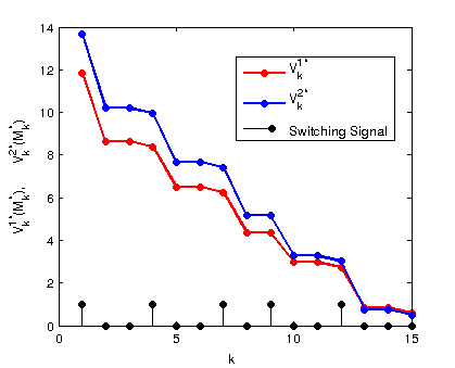
Figure 2: The red and blue lines plot 𝒱ki∗(M∗)\mathcal{V}^{i*}_{k}(M^{*}) w.r.t kk for i=1i=1 and 22 respectively. M∗M^{*} is the optimal trajectory of MkM_{k} for the optimal switching strategy (s1∗,s2∗)(s^{1*},s^{2*}). The black dots show the behavior of the optimal switching signal.
Refer to caption
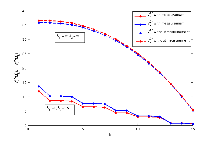
Figure 3: A comparison among the costs for the cases when costly measurements are available (λ1=1,λ2=1.5\lambda_{1}=1,\lambda_{2}=1.5) and no measurements are available (λ1=λ2=∞\lambda_{1}=\lambda_{2}=\infty)

In Figure 2, we show the optimal switching strategy Δk∗(≡Vk1∗⋅Vk2∗)\Delta_{k}^{*}(\equiv V^{1*}_{k}\cdot V^{2*}_{k}) in black dots. In a game with horizon 15, the switch was closed for 55 times. In red line, we plot the value function 𝒱k1∗(Mk∗)\mathcal{V}^{1*}_{k}(M^{*}_{k}) along the optimal trajectory of MkM_{k} determined by (21) and the optimal Δk∗\Delta_{k}^{*}. Similarly, in blue lines we plot 𝒱k2∗(Mk∗)\mathcal{V}^{2*}_{k}(M_{k}^{*}).

In Figure 3, we illustrate a comparative result for the cases when observation costs are finite (λ1=1,λ2=1.5\lambda_{1}=1,\lambda_{2}=1.5) and when observation costs are infinite (so that no observation is practically acquired). In this figure we see that even with 55 observations (out of 1515 possible), there are more than 50%50\% reductions in costs. The dotted curves in this figure also indicate the envelop of 𝒱i∗k\mathcal{V}^{i*}_{k}. In other words, all the graphs of 𝒱ki∗(Mk∗)\mathcal{V}^{i*}_{k}(M^{*}_{k}) obtained by varying the pair (λ1,λ2)(\lambda_{1},\lambda_{2}) will remain below the dotted lines shown in Figure 3.

6 Conclusion

In this work, we have considered a switched stochastic LQ game where the switching carries a finite cost. We have characterized the SPE control and switching strategies for both the players. The SPE control strategy turns out to be a linear strategy characterized by Riccati equations which do not depend on the switching strategy. The quality of state estimation depends on the switching strategy and hence the switching cost-to-go function depends on the estimation error variance. We have shown that no-switch (open switch) is always a SPE. However, at certain time instances coordinated switching is also a SPE. Moreover when both no-switch and switch are SPE, then the cost-to-go with switching is lower than the same with no-switching for both players. We studied a two-player game, however similar analysis is easily carried out for a general nn-player game.

7 Appendix

7.1 Proof of Theorem 3.1

The idea of the proof is based on backward induction. It should be noted that X^t\hat{X}_{t} satisfies the Kalman-filter like equations except the fact that the measurements are only available only through a switching and we always get noise free measurements whenever a switching is done.

We define the filtered variable as X^t=𝔼⁡[Xt|I¯t]\hat{X}_{t}=\mathbb{E}[X_{t}~|~\bar{I}_{t}] and the prediction variable as X^t+1|t=𝔼⁡[Xt+1|It]\hat{X}_{t+1|t}=\mathbb{E}[X_{t+1}|~I_{t}].

X^t|t−1=A​X^t−1+B1​Ut−11+B2​Ut−12\displaystyle\hat{X}_{t|t-1}=A\hat{X}_{t-1}+B^{1}U^{1}_{t-1}+B^{2}U^{2}_{t-1} (46)

Therefore,

X^t=(1−Δt)​X^t|t−1+Δt​Xt\hat{X}_{t}=(1-\Delta_{t})\hat{X}_{t|t-1}+\Delta_{t}X_{t}

where Δt=Vt1⋅Vt2\Delta_{t}=V^{1}_{t}\cdot V^{2}_{t}.

X^t|t−1\hat{X}_{t|t-1} satisfies the dynamics (3.1). In a compact form, one can check

X^t=A​X^t−1+B1​Ut−11+B2​Ut−12+Δt​(A​Et−1+Wt−1)\displaystyle\hat{X}_{t}=A\hat{X}_{t-1}+B^{1}U^{1}_{t-1}+B^{2}U^{2}_{t-1}+\Delta_{t}(AE_{t-1}+W_{t-1}) (47)

where Et=Xt−X^tE_{t}=X_{t}-\hat{X}_{t}. Thus it satisfies the difference equation:

Et=(1−Δt)​(A​Et−1+Wt−1)\displaystyle E_{t}=(1-\Delta_{t})(AE_{t-1}+W_{t-1}) (48)

Therefore, we can write

X^t=X^t|t−1+Δt​(A​Et−1+Wt−1)\displaystyle\hat{X}_{t}=\hat{X}_{t|t-1}+\Delta_{t}(AE_{t-1}+W_{t-1}) (49)

Let PtiP^{i}_{t} satisfy the following backward equation for i=1,2i=1,2:

Pti=\displaystyle P^{i}_{t}= Qi+Lti​Qi​i′​Lti+Ltj​Qi​j′​Ltj+(A−Bi​Lti−Bj​Ltj)′​Pt+1i​(A−Bi​Lti−Bj​Ltj)\displaystyle Q^{i}+L_{t}^{i}{{}^{\prime}}Q^{ii}L^{i}_{t}+L_{t}^{j}{{}^{\prime}}Q^{ij}L^{j}_{t}+(A-B^{i}L^{i}_{t}-B^{j}L^{j}_{t})^{\prime}P^{i}_{t+1}(A-B^{i}L^{i}_{t}-B^{j}L^{j}_{t})
PTi=\displaystyle P^{i}_{T}= Qi,\displaystyle Q^{i}, (50)

and LtiL^{i}_{t} satisfies the relation:

(Qi​i+Bi​Pti′​(I−Bj​(Qj​j+Bj​Ptj′​Bj)−1​Bj​Ptj′)​Bi)​Lt−1i\displaystyle\Big(Q^{ii}+B^{i}{{}^{\prime}}P^{i}_{t}\big(I-B^{j}(Q^{jj}+B^{j}{{}^{\prime}}P^{j}_{t}B^{j})^{-1}B^{j}{{}^{\prime}}P^{j}_{t}\big)B^{i}\Big)L^{i}_{t-1}
=Bi​Pti′​(I−Bj​(Qj​j+Bj​Ptj′​Bj)−1​Bj​Ptj′)​A\displaystyle=B^{i}{{}^{\prime}}P^{i}_{t}(I-B^{j}(Q^{jj}+B^{j}{{}^{\prime}}P^{j}_{t}B^{j})^{-1}B^{j}{{}^{\prime}}P^{j}_{t})A (51)

Let us consider the cost segment for player ii for the given switching strategy profile (s1∗,s2∗)(s^{1*},s^{2*}):

𝕁ki​(g1,g2)=\displaystyle\mathbb{J}^{i}_{k}(g^{1},g^{2})= 𝔼⁡[∑t=kTCti​(Xt,Ut1,Ut2,Vt1,Vt2)|I¯k]\displaystyle\mathbb{E}\Big[\sum_{t=k}^{T}C^{i}_{t}(X_{t},U^{1}_{t},U^{2}_{t},V^{1}_{t},V^{2}_{t})|~\bar{I}_{k}\Big]
=\displaystyle= 𝔼⁡[∑t=kTCti​(X^t,Ut1,Ut2,Vt1,Vt2)+‖Et‖Qi2|I¯k]\displaystyle\mathbb{E}\Big[\sum_{t=k}^{T}C^{i}_{t}(\hat{X}_{t},U^{1}_{t},U^{2}_{t},V^{1}_{t},V^{2}_{t})+\|E_{t}\|^{2}_{Q^{i}}|~\bar{I}_{k}\Big]
=\displaystyle= 𝔼⁡[∑t=kT−1(‖X^t‖Qi2+‖Uti‖Qi​i2+‖Utj‖Qi​j2)+‖X^T‖Qi2|I¯k]+\displaystyle\mathbb{E}\Big[\sum_{t=k}^{T-1}(\|\hat{X}_{t}\|^{2}_{Q^{i}}+\|U^{i}_{t}\|^{2}_{Q^{ii}}+\|U^{j}_{t}\|^{2}_{Q^{ij}})+\|\hat{X}_{T}\|^{2}_{Q^{i}}|~\bar{I}_{k}\Big]+
𝔼⁡[∑t=kT−1(‖Et‖Qi2+λi​Δt)+‖ET‖Qi2|I¯k]\displaystyle\mathbb{E}\Big[\sum_{t=k}^{T-1}(\|E_{t}\|^{2}_{Q^{i}}+\lambda_{i}\Delta_{t})+\|E_{T}\|^{2}_{Q^{i}}|~\bar{I}_{k}\Big] (52)

Let us denote 𝕁k1∗=ming1𝕁k1(g1,g2∗)\mathbb{J}^{1*}_{k}=\min_{g^{1}}\mathbb{J}^{1}_{k}(g^{1},g^{2*}) and g1∗=argming1𝕁k1(g1,g2∗)g^{1*}=\arg\min_{g^{1}}\mathbb{J}^{1}_{k}(g^{1},g^{2*}). Similarly we define 𝕁2∗k\mathbb{J}^{2*}_{k} and g2∗g^{2*}.

Claim 7.1

For all kk,

𝕁ki∗=𝔼[∑t=kT−1\displaystyle\mathbb{J}^{i*}_{k}=\mathbb{E}\Big[\sum_{t=k}^{T-1} (∥Et∥Qi2+Δt+1∥AEt+Wt∥Pt+1i2+λiΔt)+∥ET∥Qi2|I¯k]+∥X^k∥Pki2\displaystyle(\|E_{t}\|^{2}_{Q^{i}}+\Delta_{t+1}\|AE_{t}+W_{t}\|^{2}_{P^{i}_{t+1}}+\lambda_{i}\Delta_{t})+\|E_{T}\|^{2}_{Q^{i}}|~\bar{I}_{k}\Big]+\|\hat{X}_{k}\|_{P^{i}_{k}}^{2} (53)

where ΔT=0\Delta_{T}=0.

proof This is proven by induction. It is easy to check that conditioned under I¯t\bar{I}_{t}, EtE_{t} and X^t\hat{X}_{t} are uncorrelated.

Hence 𝔼⁡[‖Xt‖Qi2|I¯t]=𝔼⁡[‖X^t‖Qi2|I¯t]+𝔼⁡[‖Et‖Qi2|I¯t]\mathbb{E}[\|X_{t}\|^{2}_{Q^{i}}|~\bar{I}_{t}]=\mathbb{E}[\|\hat{X}_{t}\|^{2}_{Q^{i}}~|~\bar{I}_{t}]+\mathbb{E}[\|E_{t}\|^{2}_{Q^{i}}|~\bar{I}_{t}].

Therefore, at k=Tk=T, the above claim is true. At k=T−1k=T-1,

𝕁T−1i∗=mingT−1i𝔼[\displaystyle\mathbb{J}^{i*}_{T-1}=\min_{g^{i}_{T-1}}\mathbb{E}\Big[ ‖X^T−1‖Qi2+‖UT−1i‖Qi​i2+‖UT−1j‖Qi​j2+\displaystyle\|\hat{X}_{T-1}\|^{2}_{Q^{i}}+\|U^{i}_{T-1}\|^{2}_{Q^{ii}}+\|U^{j}_{T-1}\|^{2}_{Q^{ij}}+
∥X^T∥Qi2|I¯T−1]+𝔼[∥ET−1∥Qi2+λiΔT−1+∥ET∥Qi2|I¯T−1]\displaystyle\|\hat{X}_{T}\|^{2}_{Q^{i}}|~\bar{I}_{T-1}\Big]+\mathbb{E}\Big[\|E_{T-1}\|^{2}_{Q^{i}}+\lambda_{i}\Delta_{T-1}+\|E_{T}\|^{2}_{Q^{i}}|~\bar{I}_{T-1}\Big] (54)

Using X^T=A​X^T−1+B1​UT−11+B2​UT−22\hat{X}_{T}=A\hat{X}_{T-1}+B^{1}U^{1}_{T-1}+B^{2}U^{2}_{T-2}, we obtain

gi∗T−1=−LiT−1X^T−1g^{i*}_{T-1}=-L^{i}_{T-1}\hat{X}_{T-1}

Consequently, the claim holds for k=T−1k=T-1.

Let us assume that the claim holds for some k+1≤Tk+1\leq T. Then,

𝕁i∗k=\displaystyle\mathbb{J}^{i*}_{k}= 𝔼⁡[∑t=kT−1(‖Et‖Qi2+λi​Δt)+‖ET‖Qi2|I¯k]+\displaystyle\mathbb{E}\Big[\sum_{t=k}^{T-1}(\|E_{t}\|^{2}_{Q^{i}}+\lambda_{i}\Delta_{t})+\|E_{T}\|^{2}_{Q^{i}}|~\bar{I}_{k}\Big]+
mingi⁡𝔼⁡[∑t=kT−1(‖X^t‖Qi2+‖Uti‖Qi​i2+‖Utj‖Qi​j2)+‖X^T‖Qi2|I¯k]\displaystyle\min_{g^{i}}\mathbb{E}\Big[\sum_{t=k}^{T-1}(\|\hat{X}_{t}\|^{2}_{Q^{i}}+\|U^{i}_{t}\|^{2}_{Q^{ii}}+\|U^{j}_{t}\|^{2}_{Q^{ij}})+\|\hat{X}_{T}\|^{2}_{Q^{i}}|~\bar{I}_{k}\Big]
=\displaystyle= mingki𝔼[∥X^k∥Qi2+∥Uki∥Qi​i2+∥Ukj∥Qi​j2+Ji∗(k+1)|I¯k]+𝔼[∥Ek∥Qi2+λiΔk|I¯k]\displaystyle\min_{g^{i}_{k}}\mathbb{E}\Big[\|\hat{X}_{k}\|^{2}_{Q^{i}}+\|U^{i}_{k}\|^{2}_{Q^{ii}}+\|U^{j}_{k}\|^{2}_{Q^{ij}}+J^{i*}(k+1)|~\bar{I}_{k}\Big]+\mathbb{E}\Big[\|E_{k}\|^{2}_{Q^{i}}+\lambda_{i}\Delta_{k}|~\bar{I}_{k}\Big] (55)

We used that fact that I¯k⊂I¯k+1\bar{I}_{k}\subset\bar{I}_{k+1} and hence

𝔼⁡[𝔼⁡[X|Ik+1]|Ik]=𝔼⁡[X|Ik].\mathbb{E}[\mathbb{E}[X|I_{k+1}]|I_{k}]=\mathbb{E}[X|I_{k}].

Therefore using the hypothesis that the claim holds for k+1k+1, we can write (55) as:

𝕁i∗k=\displaystyle\mathbb{J}^{i*}_{k}= mingki⁡𝔼⁡[‖X^k‖Qi2+‖Uki‖Qi​i2+‖Ukj‖Qi​j2+‖X^k+1‖Pk+1i2|I¯k]\displaystyle\min_{g^{i}_{k}}\mathbb{E}\Big[\|\hat{X}_{k}\|^{2}_{Q^{i}}+\|U^{i}_{k}\|^{2}_{Q^{ii}}+\|U^{j}_{k}\|^{2}_{Q^{ij}}+\|\hat{X}_{k+1}\|^{2}_{P^{i}_{k+1}}|~\bar{I}_{k}\Big]
+𝔼⁡[∑t=kT−1(‖Et‖Qi2+λi​Δt)+‖ET‖Qi2|I¯k]+𝔼⁡[∑t=k+1T−1Δt+1​‖A​Et+Wt‖Pt+1i2|I¯k]\displaystyle+\mathbb{E}\Big[\sum_{t=k}^{T-1}(\|E_{t}\|^{2}_{Q^{i}}+\lambda_{i}\Delta_{t})+\|E_{T}\|^{2}_{Q^{i}}|~\bar{I}_{k}\Big]+\mathbb{E}\Big[\sum_{t=k+1}^{T-1}\Delta_{t+1}\|AE_{t}+W_{t}\|^{2}_{P^{i}_{t+1}}|~\bar{I}_{k}\Big] (56)

Note that,

X^k+1=A​X^k+B1​Uk1+B2​Uk2+Δk+1​(A​Ek+Wk)\hat{X}_{k+1}=A\hat{X}_{k}+B^{1}U^{1}_{k}+B^{2}U^{2}_{k}+\Delta_{k+1}(AE_{k}+W_{k})

and therefore,

𝔼⁡[‖X^k+1‖Pk+1i2|I¯k]=𝔼⁡[‖A​X^k+B1​Uk1+B2​Uk2‖Pk+1i2+Δk+1​‖(A​Ek+Wk)‖Pk+1i2|I¯k]\mathbb{E}[\|\hat{X}_{k+1}\|^{2}_{P^{i}_{k+1}}|~\bar{I}_{k}]=\mathbb{E}[\|A\hat{X}_{k}+B^{1}U^{1}_{k}+B^{2}U^{2}_{k}\|^{2}_{P^{i}_{k+1}}+\Delta_{k+1}\|(AE_{k}+W_{k})\|^{2}_{P^{i}_{k+1}}|~\bar{I}_{k}]

. As a result, we obtain,

𝕁i∗k=\displaystyle\mathbb{J}^{i*}_{k}= mingki⁡𝔼⁡[‖X^k‖Qi2+‖Uki‖Qi​i2+‖Ukj‖Qi​j2+‖A​X^k+B1​Uk1+B2​Uk2‖Pk+1i2|I¯k]\displaystyle\min_{g^{i}_{k}}\mathbb{E}\Big[\|\hat{X}_{k}\|^{2}_{Q^{i}}+\|U^{i}_{k}\|^{2}_{Q^{ii}}+\|U^{j}_{k}\|^{2}_{Q^{ij}}+\|A\hat{X}_{k}+B^{1}U^{1}_{k}+B^{2}U^{2}_{k}\|^{2}_{P^{i}_{k+1}}|~\bar{I}_{k}\Big]
+𝔼⁡[∑t=kT−1(‖Et‖Qi2+λi​Δt)+‖ET‖Qi2|I¯k]+𝔼⁡[∑t=kT−1Δt+1​‖A​Et+Wt‖Pt+1i2|I¯k]\displaystyle+\mathbb{E}\Big[\sum_{t=k}^{T-1}(\|E_{t}\|^{2}_{Q^{i}}+\lambda_{i}\Delta_{t})+\|E_{T}\|^{2}_{Q^{i}}|~\bar{I}_{k}\Big]+\mathbb{E}\Big[\sum_{t=k}^{T-1}\Delta_{t+1}\|AE_{t}+W_{t}\|^{2}_{P^{i}_{t+1}}|~\bar{I}_{k}\Big] (57)

Note that X^t\hat{X}_{t} is I¯t\bar{I}_{t} measurable for all tt. Thus, we can say from (57) that the optimal Uk1U^{1}_{k} for player 1 should be given by:

Uk1=−(Q11+B1​Pk+11′​B1)−1​B1​Pk+11′​(A​X^k+B2​Uk2)\displaystyle U^{1}_{k}=-(Q^{11}+B^{1}{{}^{\prime}}P^{1}_{k+1}B^{1})^{-1}B^{1}{{}^{\prime}}P^{1}_{k+1}(A\hat{X}_{k}+B^{2}U^{2}_{k}) (58)

Similarly, for player 22, it can be shown that the optimal Uk2U^{2}_{k} will be:

Uk2=−(Q22+B2​Pk+12′​B2)−1​B2​Pk+12′​(A​X^k+B1​Uk1)\displaystyle U^{2}_{k}=-(Q^{22}+B^{2}{{}^{\prime}}P^{2}_{k+1}B^{2})^{-1}B^{2}{{}^{\prime}}P^{2}_{k+1}(A\hat{X}_{k}+B^{1}U^{1}_{k}) (59)

Comparing the expressions for optimal UkiU^{i}_{k} and along with the definition of LkiL^{i}_{k} matrices we obtain (basically solving the two linear equations in UkiU^{i}_{k}):

Uki=gki∗(I¯k)=−LkiX^k\displaystyle U^{i}_{k}=g^{i*}_{k}(\bar{I}_{k})=-L^{i}_{k}\hat{X}_{k} (60)

Now substituting the optimal UkiU^{i}_{k} in (57), and using the definition of PkiP_{k}^{i} from (50) we get:

𝕁ki∗=𝔼[∑t=kT−1\displaystyle\mathbb{J}^{i*}_{k}=\mathbb{E}\Big[\sum_{t=k}^{T-1} (∥Et∥Qi2+Δt+1∥AEt+Wt∥Pt+1i2+λiΔt)+∥ET∥Qi2|I¯k]+∥X^k∥Pki2\displaystyle(\|E_{t}\|^{2}_{Q^{i}}+\Delta_{t+1}\|AE_{t}+W_{t}\|^{2}_{P^{i}_{t+1}}+\lambda_{i}\Delta_{t})+\|E_{T}\|^{2}_{Q^{i}}|~\bar{I}_{k}\Big]+\|\hat{X}_{k}\|_{P^{i}_{k}}^{2}

References

  • [1] D. Maity, A. Anastasopoulos, and J. S. Baras, “Linear quadratic games with costly measurements,” in Decision and Control (CDC), 2017 IEEE 56th Conference on. IEEE, 2017, accepted.
  • [2] T. Basar and G. J. Olsder, Dynamic noncooperative game theory. SIAM, 1995, vol. 200.
  • [3] J. Engwerda, LQ dynamic optimization and differential games. John Wiley & Sons, 2005.
  • [4] M. Foley and W. Schmitendorf, “On a class of nonzero-sum, linear-quadratic differential games,” Journal of Optimization Theory and Applications, vol. 7, no. 5, pp. 357–377, 1971.
  • [5] A. Weeren, J. Schumacher, and J. Engwerda, “Asymptotic analysis of linear feedback Nash equilibria in nonzero-sum linear-quadratic differential games,” Journal of Optimization Theory and Applications, vol. 101, no. 3, pp. 693–722, 1999.
  • [6] T. Basar, “On the uniqueness of the Nash solution in linear-quadratic differential games,” International Journal of Game Theory, vol. 5, no. 2-3, pp. 65–90, 1976.
  • [7] J. Cruz Jr and C. Chen, “Series Nash solution of two-person, nonzero-sum, linear-quadratic differential games,” Journal of Optimization Theory and Applications, vol. 7, no. 4, pp. 240–257, 1971.
  • [8] R. Isaacs, Differential games: a mathematical theory with applications to warfare and pursuit, control and optimization. Courier Corporation, 1999.
  • [9] P. Bernhard, “Linear-quadratic, two-person, zero-sum differential games: necessary and sufficient conditions,” Journal of Optimization Theory and Applications, vol. 27, no. 1, pp. 51–69, 1979.
  • [10] T. Basar, “A counterexample in linear-quadratic games: Existence of nonlinear Nash solutions,” Journal of Optimization Theory and Applications, vol. 14, no. 4, pp. 425–430, 1974.
  • [11] D. Maity and J. S. Baras, “Optimal strategies for stochastic linear quadratic differential games with costly information,” in Decision and Control (CDC), 2016 IEEE 55th Conference on. IEEE, 2016, pp. 276–282.
  • [12] D. Fudenberg and J. Tirole, Game theory. MIT Press, Cambridge, Massachusetts, 1991.