跳到论文正文
W Papers独立论文阅读器 arXiv:1709.06831 论文正文 计算阅读时间 · 0%
引用这篇论文根据当前论文元数据生成,正式投稿前建议核对。


License: arXiv.org perpetual non-exclusive license
arXiv:1709.06831v2 [math.CO] 15 Oct 2018

Differential transcendence & algebraicity criteria for the series counting weighted quadrant walksThanks: This project has received funding from the European Research Council (ERC) under the European Union’s Horizon 2020 research and innovation programme under the Grant Agreement No 648132 and the Grant Agreement No 759702.

Thomas Dreyfus Address: Institut de Recherche Mathématique Avancée, UMR 7501, Université de Strasbourg et CNRS, 7 rue René Descartes, 67084 Strasbourg, France Email address: dreyfus@math.unistra.fr and Kilian Raschel Address: Institut Denis Poisson, UMR 7013, Université de Tours, Université d’Orléans et CNRS, Parc de Grandmont, 37200 Tours, France Email address: raschel@math.cnrs.fr
Date: August 24, 2026
Abstract.

We consider weighted small step walks in the positive quadrant, and provide algebraicity and differential transcendence results for the underlying generating functions: we prove that depending on the probabilities of allowed steps, certain of the generating functions are algebraic over the field of rational functions, while some others do not satisfy any algebraic differential equation with rational function coefficients. Our techniques involve differential Galois theory for difference equations as well as complex analysis (Weierstrass parameterization of elliptic curves). We also extend to the weighted case many key intermediate results, as a theorem of analytic continuation of the generating functions.

Key words and phrases: 
Random walks in the quarter plane, Difference Galois theory, Elliptic functions, Transcendence, Algebraicity
2010 Mathematics Subject Classification
05A15,30D05,39A06

Introduction

Take a walk with small steps in the positive quadrant ℤ⩾02={0,1,2,…}2\mathbb{Z}_{\geqslant 0}^{2}=\{0,1,2,\ldots\}^{2}, that is a succession of points

P0,P1,…,Pk,P_{0},P_{1},\ldots,P_{k},

where each PnP_{n} lies in the quarter plane, where the moves (or steps) Pn+1−PnP_{n+1}-P_{n} belong to a finite step set 𝒮⊂{0,±1}2\mathcal{S}\subset\{0,\pm 1\}^{2} which has been chosen a priori, and the probability to move in the direction Pn+1−Pn=(i,j)P_{n+1}-P_{n}=(i,j) is equal to some weight-parameter di,jd_{i,j}, with ∑(i,j)∈𝒮di,j=1\sum_{(i,j)\in\mathcal{S}}d_{i,j}=1. The following picture is an example of such path:

𝒮={                                        }\mathcal{S}=\left\{\hbox to24.36pt{\vbox to24.36pt{\pgfpicture\makeatletter\hbox{\hskip 12.18091pt\lower-12.18091pt\hbox to0.0pt{\lxSVG@begingroup@{_scopebegin=1} \lxSVG@begingroup@{stroke=#000000} \lxSVG@begingroup@{fill=#000000} \lxSVG@setlinewidth{\the\pgflinewidth}\lxSVG@begingroup@{stroke-width=0.4pt} \lx@inpgf@ignorespaces\nullfont\hbox to0.0pt{\lxSVG@begingroup@{_scopebegin=1} {{\lx@inpgf@ignorespaces}} {}{{}}{}{{{}} {\lx@inpgf@ignorespaces}{}{\lx@inpgf@ignorespaces}{}{}{}{}{} }\lxSVG@fill\lxSVG@drawpath@unclipped{M -15.75 -15.75 M -14.64 -15.75 C -14.64 -15.14 -15.14 -14.64 -15.75 -14.64 C -16.36 -14.64 -16.85 -15.14 -16.85 -15.75 C -16.85 -16.36 -16.36 -16.85 -15.75 -16.85 C -15.14 -16.85 -14.64 -16.36 -14.64 -15.75 Z M -15.75 -15.75}{stroke:none} \lx@inpgf@ignorespaces {}{{}}{}{{{}} {\lx@inpgf@ignorespaces}{}{\lx@inpgf@ignorespaces}{}{}{}{}{} }\lxSVG@fill\lxSVG@drawpath@unclipped{M -15.75 0 M -14.64 0 C -14.64 0.61 -15.14 1.11 -15.75 1.11 C -16.36 1.11 -16.85 0.61 -16.85 0 C -16.85 -0.61 -16.36 -1.11 -15.75 -1.11 C -15.14 -1.11 -14.64 -0.61 -14.64 0 Z M -15.75 0}{stroke:none} \lx@inpgf@ignorespaces {}{{}}{}{{{}} {\lx@inpgf@ignorespaces}{}{\lx@inpgf@ignorespaces}{}{}{}{}{} }\lxSVG@fill\lxSVG@drawpath@unclipped{M -15.75 15.75 M -14.64 15.75 C -14.64 16.36 -15.14 16.85 -15.75 16.85 C -16.36 16.85 -16.85 16.36 -16.85 15.75 C -16.85 15.14 -16.36 14.64 -15.75 14.64 C -15.14 14.64 -14.64 15.14 -14.64 15.75 Z M -15.75 15.75}{stroke:none} \lx@inpgf@ignorespaces {}{{}}{}{{{}} {\lx@inpgf@ignorespaces}{}{\lx@inpgf@ignorespaces}{}{}{}{}{} }\lxSVG@fill\lxSVG@drawpath@unclipped{M 0 -15.75 M 1.11 -15.75 C 1.11 -15.14 0.61 -14.64 0 -14.64 C -0.61 -14.64 -1.11 -15.14 -1.11 -15.75 C -1.11 -16.36 -0.61 -16.85 0 -16.85 C 0.61 -16.85 1.11 -16.36 1.11 -15.75 Z M 0 -15.75}{stroke:none} \lx@inpgf@ignorespaces {}{{}}{}{{{}} {\lx@inpgf@ignorespaces}{}{\lx@inpgf@ignorespaces}{}{}{}{}{} }\lxSVG@fill\lxSVG@drawpath@unclipped{M 0 0 M 1.11 0 C 1.11 0.61 0.61 1.11 0 1.11 C -0.61 1.11 -1.11 0.61 -1.11 0 C -1.11 -0.61 -0.61 -1.11 0 -1.11 C 0.61 -1.11 1.11 -0.61 1.11 0 Z M 0 0}{stroke:none} \lx@inpgf@ignorespaces {}{{}}{}{{{}} {\lx@inpgf@ignorespaces}{}{\lx@inpgf@ignorespaces}{}{}{}{}{} }\lxSVG@fill\lxSVG@drawpath@unclipped{M 0 15.75 M 1.11 15.75 C 1.11 16.36 0.61 16.85 0 16.85 C -0.61 16.85 -1.11 16.36 -1.11 15.75 C -1.11 15.14 -0.61 14.64 0 14.64 C 0.61 14.64 1.11 15.14 1.11 15.75 Z M 0 15.75}{stroke:none} \lx@inpgf@ignorespaces {}{{}}{}{{{}} {\lx@inpgf@ignorespaces}{}{\lx@inpgf@ignorespaces}{}{}{}{}{} }\lxSVG@fill\lxSVG@drawpath@unclipped{M 15.75 -15.75 M 16.85 -15.75 C 16.85 -15.14 16.36 -14.64 15.75 -14.64 C 15.14 -14.64 14.64 -15.14 14.64 -15.75 C 14.64 -16.36 15.14 -16.85 15.75 -16.85 C 16.36 -16.85 16.85 -16.36 16.85 -15.75 Z M 15.75 -15.75}{stroke:none} \lx@inpgf@ignorespaces {}{{}}{}{{{}} {\lx@inpgf@ignorespaces}{}{\lx@inpgf@ignorespaces}{}{}{}{}{} }\lxSVG@fill\lxSVG@drawpath@unclipped{M 15.75 0 M 16.85 0 C 16.85 0.61 16.36 1.11 15.75 1.11 C 15.14 1.11 14.64 0.61 14.64 0 C 14.64 -0.61 15.14 -1.11 15.75 -1.11 C 16.36 -1.11 16.85 -0.61 16.85 0 Z M 15.75 0}{stroke:none} \lx@inpgf@ignorespaces {}{{}}{}{{{}} {\lx@inpgf@ignorespaces}{}{\lx@inpgf@ignorespaces}{}{}{}{}{} }\lxSVG@fill\lxSVG@drawpath@unclipped{M 15.75 15.75 M 16.85 15.75 C 16.85 16.36 16.36 16.85 15.75 16.85 C 15.14 16.85 14.64 16.36 14.64 15.75 C 14.64 15.14 15.14 14.64 15.75 14.64 C 16.36 14.64 16.85 15.14 16.85 15.75 Z M 15.75 15.75}{stroke:none} \lx@inpgf@ignorespaces {}{{}}{} {}{}\lxSVG@begingroup@{_scopebegin=1} \lxSVG@setlinewidth{\the\pgflinewidth}\lxSVG@begingroup@{stroke-width=0.8pt} \lx@inpgf@ignorespaces{}{{ {\lxSVG@setlinewidth{\the\pgflinewidth}\lx@inpgf@ignorespaces\lxSVG@setdash{0.0pt}\lx@inpgf@ignorespaces\lxSVG@roundcap\lx@inpgf@ignorespaces\lxSVG@roundjoin\lx@inpgf@ignorespaces{} {}{}{} {}{}{} \lxSVG@stroke}} }{}{}{{}}\lxSVG@stroke\lxSVG@drawpath@unclipped{M 0 0 L -15.05 15.05}{fill:none} {{}{{}}{}{}{{}}{{{\lx@inpgf@ignorespaces}}{{{\lx@inpgf@ignorespaces}}{\lxSVG@begingroup@{_scopebegin=1} \lxSVG@transformcm{-0.7071}{0.7071}{-0.7071}{-0.7071}{-10.87886pt}{10.87886pt}\lxSVG@begingroup@{transform=matrix(-0.7071 0.7071 -0.7071 -0.7071 -15.05 15.05)} \lxSVG@begingroup@{_scopebegin=1} \lxSVG@begingroup@{stroke-width=0.64pt} \lxSVG@begingroup@{stroke-dasharray=none,stroke-dashoffset=0.0pt} \lxSVG@begingroup@{stroke-linecap=round} \lxSVG@begingroup@{stroke-linejoin=round} \lxSVG@drawpath@unclipped{M -2.16 2.88 C -1.98 1.8 0 0.18 0.54 0 C 0 -0.18 -1.98 -1.8 -2.16 -2.88}{fill:none} \lxSVG@closescope \lxSVG@closescope }}{{\lx@inpgf@ignorespaces}}}}\lx@inpgf@ignorespaces \lxSVG@closescope {}{{}}{} {}{}\lxSVG@begingroup@{_scopebegin=1} \lxSVG@setlinewidth{\the\pgflinewidth}\lxSVG@begingroup@{stroke-width=0.8pt} \lx@inpgf@ignorespaces{}{}{}{}{{}}\lxSVG@stroke\lxSVG@drawpath@unclipped{M 0 0 L 15.05 15.05}{fill:none} {{}{{}}{}{}{{}}{{{\lx@inpgf@ignorespaces}}{{{\lx@inpgf@ignorespaces}}{\lxSVG@begingroup@{_scopebegin=1} \lxSVG@transformcm{0.7071}{0.7071}{-0.7071}{0.7071}{10.87886pt}{10.87886pt}\lxSVG@begingroup@{transform=matrix(0.7071 0.7071 -0.7071 0.7071 15.05 15.05)} \lxSVG@begingroup@{_scopebegin=1} \lxSVG@begingroup@{stroke-width=0.64pt} \lxSVG@begingroup@{stroke-dasharray=none,stroke-dashoffset=0.0pt} \lxSVG@begingroup@{stroke-linecap=round} \lxSVG@begingroup@{stroke-linejoin=round} \lxSVG@drawpath@unclipped{M -2.16 2.88 C -1.98 1.8 0 0.18 0.54 0 C 0 -0.18 -1.98 -1.8 -2.16 -2.88}{fill:none} \lxSVG@closescope \lxSVG@closescope }}{{\lx@inpgf@ignorespaces}}}}\lx@inpgf@ignorespaces \lxSVG@closescope {}{{}}{} {}{}\lxSVG@begingroup@{_scopebegin=1} \lxSVG@setlinewidth{\the\pgflinewidth}\lxSVG@begingroup@{stroke-width=0.8pt} \lx@inpgf@ignorespaces{}{}{}{}{{}}\lxSVG@stroke\lxSVG@drawpath@unclipped{M 0 0 L 15.05 -15.05}{fill:none} {{}{{}}{}{}{{}}{{{\lx@inpgf@ignorespaces}}{{{\lx@inpgf@ignorespaces}}{\lxSVG@begingroup@{_scopebegin=1} \lxSVG@transformcm{0.7071}{-0.7071}{0.7071}{0.7071}{10.87886pt}{-10.87886pt}\lxSVG@begingroup@{transform=matrix(0.7071 -0.7071 0.7071 0.7071 15.05 -15.05)} \lxSVG@begingroup@{_scopebegin=1} \lxSVG@begingroup@{stroke-width=0.64pt} \lxSVG@begingroup@{stroke-dasharray=none,stroke-dashoffset=0.0pt} \lxSVG@begingroup@{stroke-linecap=round} \lxSVG@begingroup@{stroke-linejoin=round} \lxSVG@drawpath@unclipped{M -2.16 2.88 C -1.98 1.8 0 0.18 0.54 0 C 0 -0.18 -1.98 -1.8 -2.16 -2.88}{fill:none} \lxSVG@closescope \lxSVG@closescope }}{{\lx@inpgf@ignorespaces}}}}\lx@inpgf@ignorespaces \lxSVG@closescope {}{{}}{} {}{}\lxSVG@begingroup@{_scopebegin=1} \lxSVG@setlinewidth{\the\pgflinewidth}\lxSVG@begingroup@{stroke-width=0.8pt} \lx@inpgf@ignorespaces{}{}{}{}{{}}\lxSVG@stroke\lxSVG@drawpath@unclipped{M 0 0 L 0 -14.77}{fill:none} {{}{{}}{}{}{{}}{{{\lx@inpgf@ignorespaces}}{{{\lx@inpgf@ignorespaces}}{\lxSVG@begingroup@{_scopebegin=1} \lxSVG@transformcm{0.0}{-1.0}{1.0}{0.0}{0.0pt}{-10.67091pt}\lxSVG@begingroup@{transform=matrix(0.0 -1.0 1.0 0.0 0 -14.77)} \lxSVG@begingroup@{_scopebegin=1} \lxSVG@begingroup@{stroke-width=0.64pt} \lxSVG@begingroup@{stroke-dasharray=none,stroke-dashoffset=0.0pt} \lxSVG@begingroup@{stroke-linecap=round} \lxSVG@begingroup@{stroke-linejoin=round} \lxSVG@drawpath@unclipped{M -2.16 2.88 C -1.98 1.8 0 0.18 0.54 0 C 0 -0.18 -1.98 -1.8 -2.16 -2.88}{fill:none} \lxSVG@closescope \lxSVG@closescope }}{{\lx@inpgf@ignorespaces}}}}\lx@inpgf@ignorespaces \lxSVG@closescope \lxSVG@closescope {{ {}{}{}{\lx@inpgf@ignorespaces}{\lx@inpgf@ignorespaces}}}{\lx@inpgf@ignorespaces}{\lx@inpgf@ignorespaces}\hss}\lxSVG@discardpath\lxSVG@closescope \hss}}\lxSVG@closescope\endpgfpicture}}\right\}  P0=(0,0)P_{0}=(0,0)

Such objects are very natural both in combinatorics and probability theory: they are interesting for themselves and also because they are strongly related to other discrete structures, see [BMM10, DW15] and references therein.

Our main object of investigation is the probability

(1) ℙ[P0⟶k(i,j)]\mathbb{P}[P_{0}{\stackrel{{\scriptstyle k}}{{\longrightarrow}}}(i,j)]

that the walk started at P0P_{0} be at some generic position (i,j)(i,j) after the kkth step, with all intermediate points PnP_{n} remaining in the cone. More specifically we shall turn our attention to the generating function (or counting function)

(2) Q(x,y;t)=∑i,j,k⩾0ℙ[P0⟶k(i,j)]xiyjtk.Q(x,y;t)=\sum_{i,j,k\geqslant 0}\mathbb{P}[P_{0}\stackrel{{\scriptstyle k}}{{\longrightarrow}}(i,j)]x^{i}y^{j}t^{k}.

We are interesting in classifying the algebraic nature of the above series: to which of the following classes does the function (2) belong to:

(3) {rational}⊂{algebraic}⊂{holonomic}⊂{differentially algebraic}v.s.{differentially transcendental}​?\{\text{rational}\}\subset\{\text{algebraic}\}\subset\{\text{holonomic}\}\subset\{\text{differentially algebraic}\}\\ \text{v.s.}\quad\{\text{differentially transcendental}\}?

Rational and algebraic functions are classical notions. By Q⁡(x,y,t)Q(x,y;t) holonomic (resp. differentially algebraic) we mean that all of x↦Q⁡(x,y,t)x\mapsto Q(x,y;t), y↦Q⁡(x,y,t)y\mapsto Q(x,y;t) and t↦Q⁡(x,y,t)t\mapsto Q(x,y;t) satisfy a linear (resp. algebraic) differential equation with coefficients in ℂ⁡(x)\mathbb{C}(x), ℂ⁡(y)\mathbb{C}(y) and ℂ⁡(t)\mathbb{C}(t), respectively; see Definition 30 for a more precise statement. We say that Q⁡(x,y,t)Q(x,y;t) is differentially transcendental if it is not differentially algebraic. Our main results give sufficient conditions on the weights di,jd_{i,j} to characterize the algebraic nature (3) of the counting function (2).

Motivations to consider models of weighted walks

In this article we shall go beyond the classical hypothesis consisting in studying unweighted walks, that is walks with di,j=1/|𝒮|d_{i,j}=1/|\mathcal{S}| for all (i,j)∈𝒮(i,j)\in\mathcal{S}. Indeed, motivations to consider weighted models are multiple: first, they offer a natural framework to generalize the numerous results established for unweighted lattice walks, see our bibliography for a nonexhaustive list of works concerning unweighted quadrant walks, especially [BMM10, BRS14, BK10, DHRS18, FR10, KR12, KR15, Mis09, MM14, MR09]. Second, some models of unweighted walks in dimension 33 happen to be, after projection, equivalent to models of 2D weighted walks [BBMKM16]. Needless to mention that lattice walks in 3D represent a particularly challenging topic, see [BBMKM16, DHW16]. Third, these models with weights yield results in probability theory, where the hypothesis to have only uniform probabilities (case of unweighted lattice walks) is too restrictive. Fourth, since there exist infinitely many weighted models (compare with only 7979 unweighted small step models!), case-by-case reasonings should be excluded, and in some sense only intrinsic arguments merge up, like in [FIM99, DHRS17].

Literature

There is a large literature on (mostly unweighted) walks in the quarter plane, focusing on various probabilistic and combinatorial aspects. Two main questions have attracted the attention of the mathematical community:

  • •

    finding a closed-form expression for the probability (1), or equivalently for the series (2);

  • •

    characterizing the algebraic nature of the series (2), according to the classes depicted in (3).

The first question, combinatorial in nature, should not put the second one in the shade: knowing the nature of Q⁡(x,y,t)Q(x,y;t) has consequences on the asymptotic behavior of the coefficients, and further allows to apprehend the complexity of these lattice paths problems (to illustrate this fact, let us remind that unconstrained walks are associated with rational generating functions, while walks confined to a half-plane admit algebraic counting functions [BMP00]). This is the second question that we shall consider in the present work.

To summarize the main results obtained so far in the literature, one can say that for unweighted quadrant models, the generating function (2) is holonomic (third class of functions in (3)) if and only if a certain group of transformations (simply related to the weights, see (30)) is finite; note that models having a finite group are models to which a generalization of the well-known reflection principle applies. This is a very satisfactory result, as it connects combinatorial aspects to geometric features. Moreover, there are various tools for verifying whether given parameters lead to a finite or infinite group [BMM10, FR10, KY15].

Going back to the algebraic nature of the counting function, the pioneering result is [FIM99] (Chapter 4 of that book), which states that if the group is finite, the function (2) is holonomic, and even algebraic provided that some further condition be satisfied. Then Mishna [Mis09], Mishna and Rechnitzer [MR09], Mishna and Melczer [MM14] observed that there exist infinite group models such that the series is nonholonomic. Bousquet-Mélou and Mishna [BMM10], Bostan and Kauers [BK10] proved that the series is holonomic for all unweighted quadrant models with finite group. The converse statement is shown in [KR12, BRS14]: for all infinite group models, the series is nonholonomic. The combination of all these works yields the aforementioned equivalence between finite group and holonomic generating function.

The question of differential algebraicity was approached more recently. Bernardi, Bousquet-Mélou and the second author of the present paper showed [BBMR17] that despite being nonholonomic, 99 unweighted quadrant models are differentially algebraic. In [DHRS18, DHRS17], the first author of this paper, Hardouin, Roques and Singer proved that all 4747 remaining infinite group models are differentially transcendental. See [FR10, KY15, DHW16] for related studies.

Main results

The above recap shows how actively the combinatorial community took possession of these quadrant walk problems. It also illustrates that within a relatively small class of problems (only 7979 unweighted different models!), there exists a remarkable variety of behaviors. This certainly explains the vivid interest in this model.

In this article we bring three main contributions, building on the recent works [FIM99, KR12, KR15, DHR18, DHRS18, DHRS17] and mixing techniques coming from complex analysis and Galois theory. The first contribution is about the techniques: along the way of proving our other contributions we generalize a certain number of results of [FIM99] (stationary probabilistic case) and [KR12] (unweighted combinatorial case). In particular we prove an analytic continuation result of the generating functions to a certain elliptic curve, see Theorem 28.

The differential Galois results of [DHRS18] are applied in the setting of unweighted walks with infinite group, and the only serious obstruction to their extension to the weighted case was to prove the analytic continuation result of Theorem 28. Accordingly the results of [DHRS18] may be extended to the weighted case. Our second contribution is to provide differential transcendence sufficient conditions for infinite group weighted walks, see Theorems 35, 39 and 41. Those are consequences of a more general result, Proposition 32, coming from [DHR18], which is a criteria (i.e., a necessary and sufficient condition) for differential transcendence. The latter is however not totally explicit in terms of the parameters di,jd_{i,j}, contrary to the (easily verified) sufficient conditions. Note that the proofs here are omitted since they are similar to [DHRS18].

Our third result is about models having a finite group. Theorem 42 and Corollary 43 show that the generating functions are then holonomic, and even algebraic if and only if a certain quantity vanishes (namely, the alternating sum of the monomial x​yxy under the orbit of the group).

Structure of the paper

  • •

    Section 1: statement of the kernel functional equation (6) satisfied by the generating function, study of the zero set defined by the kernel. Results in that section generalize results in [FIM99, KR12], at several places with new and minimal proofs.

  • •

    Section 2: elliptic parametrization of the zero set of the kernel and continuation of the generating functions. Results in this section are importantly used in Sections 3 and 4.

  • •

    Section 3: statement of Theorems 35, 39 and 41, giving sufficient conditions for differential transcendence of the counting series.

  • •

    Section 4: Theorem 42 and Corollary 43 on algebraicity criteria for the generating functions in the finite group case.

Acknowledgements. We would like to thank Alin Bostan, Charlotte Hardouin, Manuel Kauers, Julien Roques and Michael Singer for discussions and support of this work. We express our deepest gratitude to the anonymous referee, whose numerous remarks and suggestions have led us to greatly improve our work.

1. Kernel of the walk

1.1. Functional equation

Weighted walks with small steps in the quarter plane are sums of steps taken in a step set 𝒮\mathcal{S}, itself being a subset of {           ,           ,           ,           ,           ,           ,           ,           }\{\hbox to9.34pt{\vbox to0.8pt{\pgfpicture\makeatletter\hbox{\hskip 8.9359pt\lower-0.4pt\hbox to0.0pt{\lxSVG@begingroup@{_scopebegin=1} \lxSVG@begingroup@{stroke=#000000} \lxSVG@begingroup@{fill=#000000} \lxSVG@setlinewidth{\the\pgflinewidth}\lxSVG@begingroup@{stroke-width=0.4pt} \lx@inpgf@ignorespaces\nullfont\hbox to0.0pt{\lxSVG@begingroup@{_scopebegin=1} {{\lx@inpgf@ignorespaces}} ; {}{{}}{} {}{}\lxSVG@begingroup@{_scopebegin=1} \lxSVG@setlinewidth{\the\pgflinewidth}\lxSVG@begingroup@{stroke-width=0.8pt} \lx@inpgf@ignorespaces{}{}{}{}{{}}\lxSVG@stroke\lxSVG@drawpath@unclipped{M 0 0 L -10.83 0}{fill:none} {{}{{}}{}{}{{}}{{{\lx@inpgf@ignorespaces}}{{{\lx@inpgf@ignorespaces}}{\lxSVG@begingroup@{_scopebegin=1} \lxSVG@transformcm{-1.0}{0.0}{0.0}{-1.0}{-7.8259pt}{0.0pt}\lxSVG@begingroup@{transform=matrix(-1.0 0.0 0.0 -1.0 -10.83 0)} \lxSVG@begingroup@{_scopebegin=1} \lxSVG@begingroup@{stroke-width=0.64pt} \lxSVG@begingroup@{stroke-dasharray=none,stroke-dashoffset=0.0pt} \lxSVG@begingroup@{stroke-linecap=round} \lxSVG@begingroup@{stroke-linejoin=round} \lxSVG@drawpath@unclipped{M -2.16 2.88 C -1.98 1.8 0 0.18 0.54 0 C 0 -0.18 -1.98 -1.8 -2.16 -2.88}{fill:none} \lxSVG@closescope \lxSVG@closescope }}{{\lx@inpgf@ignorespaces}}}}\lx@inpgf@ignorespaces \lxSVG@closescope \lxSVG@closescope {\lx@inpgf@ignorespaces}{\lx@inpgf@ignorespaces}{\lx@inpgf@ignorespaces}\hss}\lxSVG@discardpath\lxSVG@closescope \hss}}\lxSVG@closescope\endpgfpicture}},\hbox to9.34pt{\vbox to9.34pt{\pgfpicture\makeatletter\hbox{\hskip 8.9359pt\lower-0.4pt\hbox to0.0pt{\lxSVG@begingroup@{_scopebegin=1} \lxSVG@begingroup@{stroke=#000000} \lxSVG@begingroup@{fill=#000000} \lxSVG@setlinewidth{\the\pgflinewidth}\lxSVG@begingroup@{stroke-width=0.4pt} \lx@inpgf@ignorespaces\nullfont\hbox to0.0pt{\lxSVG@begingroup@{_scopebegin=1} {{\lx@inpgf@ignorespaces}} ; {}{{}}{} {}{}\lxSVG@begingroup@{_scopebegin=1} \lxSVG@setlinewidth{\the\pgflinewidth}\lxSVG@begingroup@{stroke-width=0.8pt} \lx@inpgf@ignorespaces{}{}{}{}{{}}\lxSVG@stroke\lxSVG@drawpath@unclipped{M 0 0 L -11.12 11.12}{fill:none} {{}{{}}{}{}{{}}{{{\lx@inpgf@ignorespaces}}{{{\lx@inpgf@ignorespaces}}{\lxSVG@begingroup@{_scopebegin=1} \lxSVG@transformcm{-0.7071}{0.7071}{-0.7071}{-0.7071}{-8.03384pt}{8.03384pt}\lxSVG@begingroup@{transform=matrix(-0.7071 0.7071 -0.7071 -0.7071 -11.12 11.12)} \lxSVG@begingroup@{_scopebegin=1} \lxSVG@begingroup@{stroke-width=0.64pt} \lxSVG@begingroup@{stroke-dasharray=none,stroke-dashoffset=0.0pt} \lxSVG@begingroup@{stroke-linecap=round} \lxSVG@begingroup@{stroke-linejoin=round} \lxSVG@drawpath@unclipped{M -2.16 2.88 C -1.98 1.8 0 0.18 0.54 0 C 0 -0.18 -1.98 -1.8 -2.16 -2.88}{fill:none} \lxSVG@closescope \lxSVG@closescope }}{{\lx@inpgf@ignorespaces}}}}\lx@inpgf@ignorespaces \lxSVG@closescope \lxSVG@closescope {\lx@inpgf@ignorespaces}{\lx@inpgf@ignorespaces}{\lx@inpgf@ignorespaces}\hss}\lxSVG@discardpath\lxSVG@closescope \hss}}\lxSVG@closescope\endpgfpicture}},\hbox to0.8pt{\vbox to9.34pt{\pgfpicture\makeatletter\hbox{\hskip 0.4pt\lower-0.4pt\hbox to0.0pt{\lxSVG@begingroup@{_scopebegin=1} \lxSVG@begingroup@{stroke=#000000} \lxSVG@begingroup@{fill=#000000} \lxSVG@setlinewidth{\the\pgflinewidth}\lxSVG@begingroup@{stroke-width=0.4pt} \lx@inpgf@ignorespaces\nullfont\hbox to0.0pt{\lxSVG@begingroup@{_scopebegin=1} {{\lx@inpgf@ignorespaces}} ; {}{{}}{} {}{}\lxSVG@begingroup@{_scopebegin=1} \lxSVG@setlinewidth{\the\pgflinewidth}\lxSVG@begingroup@{stroke-width=0.8pt} \lx@inpgf@ignorespaces{}{}{}{}{{}}\lxSVG@stroke\lxSVG@drawpath@unclipped{M 0 0 L 0 10.83}{fill:none} {{}{{}}{}{}{{}}{{{\lx@inpgf@ignorespaces}}{{{\lx@inpgf@ignorespaces}}{\lxSVG@begingroup@{_scopebegin=1} \lxSVG@transformcm{0.0}{1.0}{-1.0}{0.0}{0.0pt}{7.8259pt}\lxSVG@begingroup@{transform=matrix(0.0 1.0 -1.0 0.0 0 10.83)} \lxSVG@begingroup@{_scopebegin=1} \lxSVG@begingroup@{stroke-width=0.64pt} \lxSVG@begingroup@{stroke-dasharray=none,stroke-dashoffset=0.0pt} \lxSVG@begingroup@{stroke-linecap=round} \lxSVG@begingroup@{stroke-linejoin=round} \lxSVG@drawpath@unclipped{M -2.16 2.88 C -1.98 1.8 0 0.18 0.54 0 C 0 -0.18 -1.98 -1.8 -2.16 -2.88}{fill:none} \lxSVG@closescope \lxSVG@closescope }}{{\lx@inpgf@ignorespaces}}}}\lx@inpgf@ignorespaces \lxSVG@closescope \lxSVG@closescope {\lx@inpgf@ignorespaces}{\lx@inpgf@ignorespaces}{\lx@inpgf@ignorespaces}\hss}\lxSVG@discardpath\lxSVG@closescope \hss}}\lxSVG@closescope\endpgfpicture}},\hbox to9.34pt{\vbox to9.34pt{\pgfpicture\makeatletter\hbox{\hskip 0.4pt\lower-0.4pt\hbox to0.0pt{\lxSVG@begingroup@{_scopebegin=1} \lxSVG@begingroup@{stroke=#000000} \lxSVG@begingroup@{fill=#000000} \lxSVG@setlinewidth{\the\pgflinewidth}\lxSVG@begingroup@{stroke-width=0.4pt} \lx@inpgf@ignorespaces\nullfont\hbox to0.0pt{\lxSVG@begingroup@{_scopebegin=1} {{\lx@inpgf@ignorespaces}} ; {}{{}}{} {}{}\lxSVG@begingroup@{_scopebegin=1} \lxSVG@setlinewidth{\the\pgflinewidth}\lxSVG@begingroup@{stroke-width=0.8pt} \lx@inpgf@ignorespaces{}{}{}{}{{}}\lxSVG@stroke\lxSVG@drawpath@unclipped{M 0 0 L 11.12 11.12}{fill:none} {{}{{}}{}{}{{}}{{{\lx@inpgf@ignorespaces}}{{{\lx@inpgf@ignorespaces}}{\lxSVG@begingroup@{_scopebegin=1} \lxSVG@transformcm{0.7071}{0.7071}{-0.7071}{0.7071}{8.03384pt}{8.03384pt}\lxSVG@begingroup@{transform=matrix(0.7071 0.7071 -0.7071 0.7071 11.12 11.12)} \lxSVG@begingroup@{_scopebegin=1} \lxSVG@begingroup@{stroke-width=0.64pt} \lxSVG@begingroup@{stroke-dasharray=none,stroke-dashoffset=0.0pt} \lxSVG@begingroup@{stroke-linecap=round} \lxSVG@begingroup@{stroke-linejoin=round} \lxSVG@drawpath@unclipped{M -2.16 2.88 C -1.98 1.8 0 0.18 0.54 0 C 0 -0.18 -1.98 -1.8 -2.16 -2.88}{fill:none} \lxSVG@closescope \lxSVG@closescope }}{{\lx@inpgf@ignorespaces}}}}\lx@inpgf@ignorespaces \lxSVG@closescope \lxSVG@closescope {\lx@inpgf@ignorespaces}{\lx@inpgf@ignorespaces}{\lx@inpgf@ignorespaces}\hss}\lxSVG@discardpath\lxSVG@closescope \hss}}\lxSVG@closescope\endpgfpicture}},\hbox to9.34pt{\vbox to0.8pt{\pgfpicture\makeatletter\hbox{\hskip 0.4pt\lower-0.4pt\hbox to0.0pt{\lxSVG@begingroup@{_scopebegin=1} \lxSVG@begingroup@{stroke=#000000} \lxSVG@begingroup@{fill=#000000} \lxSVG@setlinewidth{\the\pgflinewidth}\lxSVG@begingroup@{stroke-width=0.4pt} \lx@inpgf@ignorespaces\nullfont\hbox to0.0pt{\lxSVG@begingroup@{_scopebegin=1} {{\lx@inpgf@ignorespaces}} ; {}{{}}{} {}{}\lxSVG@begingroup@{_scopebegin=1} \lxSVG@setlinewidth{\the\pgflinewidth}\lxSVG@begingroup@{stroke-width=0.8pt} \lx@inpgf@ignorespaces{}{}{}{}{{}}\lxSVG@stroke\lxSVG@drawpath@unclipped{M 0 0 L 10.83 0}{fill:none} {{}{{}}{}{}{{}}{{{\lx@inpgf@ignorespaces}}{{{\lx@inpgf@ignorespaces}}{\lxSVG@begingroup@{_scopebegin=1} \lxSVG@transformcm{1.0}{0.0}{0.0}{1.0}{7.8259pt}{0.0pt}\lxSVG@begingroup@{transform=matrix(1.0 0.0 0.0 1.0 10.83 0)} \lxSVG@begingroup@{_scopebegin=1} \lxSVG@begingroup@{stroke-width=0.64pt} \lxSVG@begingroup@{stroke-dasharray=none,stroke-dashoffset=0.0pt} \lxSVG@begingroup@{stroke-linecap=round} \lxSVG@begingroup@{stroke-linejoin=round} \lxSVG@drawpath@unclipped{M -2.16 2.88 C -1.98 1.8 0 0.18 0.54 0 C 0 -0.18 -1.98 -1.8 -2.16 -2.88}{fill:none} \lxSVG@closescope \lxSVG@closescope }}{{\lx@inpgf@ignorespaces}}}}\lx@inpgf@ignorespaces \lxSVG@closescope \lxSVG@closescope {\lx@inpgf@ignorespaces}{\lx@inpgf@ignorespaces}{\lx@inpgf@ignorespaces}\hss}\lxSVG@discardpath\lxSVG@closescope \hss}}\lxSVG@closescope\endpgfpicture}},\hbox to9.34pt{\vbox to9.34pt{\pgfpicture\makeatletter\hbox{\hskip 0.4pt\lower-8.9359pt\hbox to0.0pt{\lxSVG@begingroup@{_scopebegin=1} \lxSVG@begingroup@{stroke=#000000} \lxSVG@begingroup@{fill=#000000} \lxSVG@setlinewidth{\the\pgflinewidth}\lxSVG@begingroup@{stroke-width=0.4pt} \lx@inpgf@ignorespaces\nullfont\hbox to0.0pt{\lxSVG@begingroup@{_scopebegin=1} {{\lx@inpgf@ignorespaces}} ; {}{{}}{} {}{}\lxSVG@begingroup@{_scopebegin=1} \lxSVG@setlinewidth{\the\pgflinewidth}\lxSVG@begingroup@{stroke-width=0.8pt} \lx@inpgf@ignorespaces{}{}{}{}{{}}\lxSVG@stroke\lxSVG@drawpath@unclipped{M 0 0 L 11.12 -11.12}{fill:none} {{}{{}}{}{}{{}}{{{\lx@inpgf@ignorespaces}}{{{\lx@inpgf@ignorespaces}}{\lxSVG@begingroup@{_scopebegin=1} \lxSVG@transformcm{0.7071}{-0.7071}{0.7071}{0.7071}{8.03384pt}{-8.03384pt}\lxSVG@begingroup@{transform=matrix(0.7071 -0.7071 0.7071 0.7071 11.12 -11.12)} \lxSVG@begingroup@{_scopebegin=1} \lxSVG@begingroup@{stroke-width=0.64pt} \lxSVG@begingroup@{stroke-dasharray=none,stroke-dashoffset=0.0pt} \lxSVG@begingroup@{stroke-linecap=round} \lxSVG@begingroup@{stroke-linejoin=round} \lxSVG@drawpath@unclipped{M -2.16 2.88 C -1.98 1.8 0 0.18 0.54 0 C 0 -0.18 -1.98 -1.8 -2.16 -2.88}{fill:none} \lxSVG@closescope \lxSVG@closescope }}{{\lx@inpgf@ignorespaces}}}}\lx@inpgf@ignorespaces \lxSVG@closescope \lxSVG@closescope {\lx@inpgf@ignorespaces}{\lx@inpgf@ignorespaces}{\lx@inpgf@ignorespaces}\hss}\lxSVG@discardpath\lxSVG@closescope \hss}}\lxSVG@closescope\endpgfpicture}},\hbox to0.8pt{\vbox to9.34pt{\pgfpicture\makeatletter\hbox{\hskip 0.4pt\lower-8.9359pt\hbox to0.0pt{\lxSVG@begingroup@{_scopebegin=1} \lxSVG@begingroup@{stroke=#000000} \lxSVG@begingroup@{fill=#000000} \lxSVG@setlinewidth{\the\pgflinewidth}\lxSVG@begingroup@{stroke-width=0.4pt} \lx@inpgf@ignorespaces\nullfont\hbox to0.0pt{\lxSVG@begingroup@{_scopebegin=1} {{\lx@inpgf@ignorespaces}} ; {}{{}}{} {}{}\lxSVG@begingroup@{_scopebegin=1} \lxSVG@setlinewidth{\the\pgflinewidth}\lxSVG@begingroup@{stroke-width=0.8pt} \lx@inpgf@ignorespaces{}{}{}{}{{}}\lxSVG@stroke\lxSVG@drawpath@unclipped{M 0 0 L 0 -10.83}{fill:none} {{}{{}}{}{}{{}}{{{\lx@inpgf@ignorespaces}}{{{\lx@inpgf@ignorespaces}}{\lxSVG@begingroup@{_scopebegin=1} \lxSVG@transformcm{0.0}{-1.0}{1.0}{0.0}{0.0pt}{-7.8259pt}\lxSVG@begingroup@{transform=matrix(0.0 -1.0 1.0 0.0 0 -10.83)} \lxSVG@begingroup@{_scopebegin=1} \lxSVG@begingroup@{stroke-width=0.64pt} \lxSVG@begingroup@{stroke-dasharray=none,stroke-dashoffset=0.0pt} \lxSVG@begingroup@{stroke-linecap=round} \lxSVG@begingroup@{stroke-linejoin=round} \lxSVG@drawpath@unclipped{M -2.16 2.88 C -1.98 1.8 0 0.18 0.54 0 C 0 -0.18 -1.98 -1.8 -2.16 -2.88}{fill:none} \lxSVG@closescope \lxSVG@closescope }}{{\lx@inpgf@ignorespaces}}}}\lx@inpgf@ignorespaces \lxSVG@closescope \lxSVG@closescope {\lx@inpgf@ignorespaces}{\lx@inpgf@ignorespaces}{\lx@inpgf@ignorespaces}\hss}\lxSVG@discardpath\lxSVG@closescope \hss}}\lxSVG@closescope\endpgfpicture}},\hbox to9.34pt{\vbox to9.34pt{\pgfpicture\makeatletter\hbox{\hskip 8.9359pt\lower-8.9359pt\hbox to0.0pt{\lxSVG@begingroup@{_scopebegin=1} \lxSVG@begingroup@{stroke=#000000} \lxSVG@begingroup@{fill=#000000} \lxSVG@setlinewidth{\the\pgflinewidth}\lxSVG@begingroup@{stroke-width=0.4pt} \lx@inpgf@ignorespaces\nullfont\hbox to0.0pt{\lxSVG@begingroup@{_scopebegin=1} {{\lx@inpgf@ignorespaces}} ; {}{{}}{} {}{}\lxSVG@begingroup@{_scopebegin=1} \lxSVG@setlinewidth{\the\pgflinewidth}\lxSVG@begingroup@{stroke-width=0.8pt} \lx@inpgf@ignorespaces{}{}{}{}{{}}\lxSVG@stroke\lxSVG@drawpath@unclipped{M 0 0 L -11.12 -11.12}{fill:none} {{}{{}}{}{}{{}}{{{\lx@inpgf@ignorespaces}}{{{\lx@inpgf@ignorespaces}}{\lxSVG@begingroup@{_scopebegin=1} \lxSVG@transformcm{-0.7071}{-0.7071}{0.7071}{-0.7071}{-8.03384pt}{-8.03384pt}\lxSVG@begingroup@{transform=matrix(-0.7071 -0.7071 0.7071 -0.7071 -11.12 -11.12)} \lxSVG@begingroup@{_scopebegin=1} \lxSVG@begingroup@{stroke-width=0.64pt} \lxSVG@begingroup@{stroke-dasharray=none,stroke-dashoffset=0.0pt} \lxSVG@begingroup@{stroke-linecap=round} \lxSVG@begingroup@{stroke-linejoin=round} \lxSVG@drawpath@unclipped{M -2.16 2.88 C -1.98 1.8 0 0.18 0.54 0 C 0 -0.18 -1.98 -1.8 -2.16 -2.88}{fill:none} \lxSVG@closescope \lxSVG@closescope }}{{\lx@inpgf@ignorespaces}}}}\lx@inpgf@ignorespaces \lxSVG@closescope \lxSVG@closescope {\lx@inpgf@ignorespaces}{\lx@inpgf@ignorespaces}{\lx@inpgf@ignorespaces}\hss}\lxSVG@discardpath\lxSVG@closescope \hss}}\lxSVG@closescope\endpgfpicture}}\}, or alternatively

Steps will be identified with pairs (i,j)∈{0,±1}2\{(0,0)}(i,j)\in\{0,\pm 1\}^{2}\backslash\{(0,0)\}. For (i,j)∈{0,±1}2(i,j)\in\{0,\pm 1\}^{2}, let di,j∈[0,1]d_{i,j}\in[0,1] with ∑di,j=1\sum d_{i,j}=1. We consider quadrant walks starting from P0=(0,0)∈ℤ⩾02P_{0}=(0,0)\in\mathbb{Z}_{\geqslant 0}^{2}, which at each time move in the direction (i,j)(i,j) (resp. stay at the same position) with probability di,jd_{i,j} (resp. d0,0d_{0,0}). A walk will be called unweighted if d0,0=0d_{0,0}=0 and if in addition all nonzero di,jd_{i,j} take the same value.

As said in the introduction, we will mainly focus on the probability ℙ[P0⟶k(i,j)]\mathbb{P}[P_{0}{\stackrel{{\scriptstyle k}}{{\longrightarrow}}}(i,j)] that the walk be at position (i,j)(i,j) after kk steps, starting from P0P_{0} and with all intermediate points P1,…,Pk−1P_{1},\ldots,P_{k-1} in the quarter plane. The corresponding trivariate generating function Q⁡(x,y,t)Q(x,y;t) is defined in (2). Being the generating function of probabilities, Q⁡(x,y,t)Q(x,y;t) converges for all (x,y,t)∈ℂ3(x,y,t)\in\mathbb{C}^{3} such that |x|,|y|⩽1|x|,|y|\leqslant 1 and |t|<1|t|<1. Note that in several papers, as in [BMM10], it is not assumed that ∑di,j=1\sum d_{i,j}=1. However, after a rescaling of the tt-variable, we may always reduce to this case.

The kernel of the walk is the polynomial defined by K⁡(x,y,t):=x​y​(1−t​S​(x,y)),K(x,y;t):=xy(1-tS(x,y)), where S⁡(x,y)S(x,y) denotes the jump polynomial

(4) S⁡(x,y)=∑(i,j)∈{0,±1}2di,j​xi​yj=A−1​(x)​1y+A0​(x)+A1​(x)​y=B−1​(y)​1x+B0​(y)+B1​(y)​x,S(x,y)=\sum_{(i,j)\in\{0,\pm 1\}^{2}}d_{i,j}x^{i}y^{j}=A_{-1}(x)\frac{1}{y}+A_{0}(x)+A_{1}(x)y=B_{-1}(y)\frac{1}{x}+B_{0}(y)+B_{1}(y)x,

and Ai​(x)∈x−1​ℝ​[x]A_{i}(x)\in x^{-1}\mathbb{R}[x], Bi​(y)∈y−1​ℝ​[y]B_{i}(y)\in y^{-1}\mathbb{R}[y]. Define further

(5) F1​(x,t):=K⁡(x,0,t)​Q​(x,0,t)andF2​(y,t):=K⁡(0,y,t)​Q​(0,y,t).F^{1}(x;t):=K(x,0;t)Q(x,0;t)\quad\text{and}\quad F^{2}(y;t):=K(0,y;t)Q(0,y;t).

The following is an adaptation of [BMM10, Lemma 4] to our context; the proof is omitted since it is exactly the same as in [BMM10, DHRS17].

Lemma 1.

The generating function Q⁡(x,y,t)Q(x,y;t) introduced in (2) satisfies the functional equation

(6) K⁡(x,y,t)​Q​(x,y,t)=F1​(x,t)+F2​(y,t)−K⁡(0,0,t)​Q​(0,0,t)+x​y.K(x,y;t)Q(x,y;t)=F^{1}(x;t)+F^{2}(y;t)-K(0,0;t)Q(0,0;t)+xy.

1.2. Nondegenerate walks

From now, let us fix t∈(0,1)t\in(0,1). The kernel curve E¯t\overline{E}_{t} is defined as the zero set in ℙ1​(ℂ)2\mathbb{P}^{1}(\mathbb{C})^{2} of the homogeneous polynomial

(7) K¯​(x0,x1,y0,y1,t)=x0​x1​y0​y1−t​∑i,j=02di−1,j−1​x0i​x12−i​y0j​y12−j,\overline{K}(x_{0},x_{1},y_{0},y_{1};t)=x_{0}x_{1}y_{0}y_{1}-t\sum_{i,j=0}^{2}d_{i-1,j-1}x_{0}^{i}x_{1}^{2-i}y_{0}^{j}y_{1}^{2-j},

namely,

(8) E¯t={([x0:x1],[y0:y1])∈ℙ1(ℂ)2:K¯(x0,x1,y0,y1;t)=0}.\overline{E}_{t}=\{([x_{0}\!:\!x_{1}],[y_{0}\!:\!y_{1}])\in\mathbb{P}^{1}(\mathbb{C})^{2}:\overline{K}(x_{0},x_{1},y_{0},y_{1};t)=0\}.

Working in ℙ1​(ℂ)\mathbb{P}^{1}(\mathbb{C}) rather than on ℂ\mathbb{C} appears to be particularly convenient and allows avoiding tedious discussions (as in particular on the number of branch points, see [KR12, Section 2.1]). To simplify our notation, for x=[x0:x1]x=[x_{0}\!:\!x_{1}] and y=[y0:y1]∈ℙ1(ℂ)y=[y_{0}\!:\!y_{1}]\in\mathbb{P}^{1}(\mathbb{C}), we shall alternatively write K¯​(x,y,t)\overline{K}(x,y;t), K¯​(x,y0,y1,t)\overline{K}(x,y_{0},y_{1};t) and K¯​(x0,x1,y,t)\overline{K}(x_{0},x_{1},y;t) instead of K¯​(x0,x1,y0,y1,t)\overline{K}(x_{0},x_{1},y_{0},y_{1};t).

Following [FIM99] we introduce the concept of degenerate model.

Definition 2.

A walk is called degenerate if one of the following assertions holds:

  • •

    (x,y)↦K⁡(x,y,t)(x,y)\mapsto K(x,y;t) is reducible over ℂ⁡[x,y]\mathbb{C}[x,y];

  • •

    (x,y)↦K⁡(x,y,t)(x,y)\mapsto K(x,y;t) has not bidegree (2,2)(2,2), that is xx- or yy-degree smaller than or equal to 11.

By (4) or (7), the terms in x2x^{2} (resp. y2y^{2}) in K⁡(x,y,t)/tK(x,y;t)/t form a polynomial of degree at most two in yy (resp. xx), which does not depend upon tt. So (x,y)↦K⁡(x,y,t)(x,y)\mapsto K(x,y;t) has not bidegree (2,2)(2,2) for one particular t∈ℂ∗t\in\mathbb{C}^{*} if and only if it has not bidegree (2,2)(2,2) for every value of t∈ℂ∗t\in\mathbb{C}^{*}.

On the other hand, the polynomial K⁡(x,y,t)K(x,y;t) might be irreducible for some values of t∈ℂ∗t\in\mathbb{C}^{*} and reducible for other values of tt, so that the notion of degenerate model a priori depends on tt. However, we will see in Proposition 3 and its proof that a walk is degenerate for a specific value of t∈(0,1)t\in(0,1) if and only if it is degenerate for every t∈(0,1)t\in(0,1), so that the values of tt yielding a factorization of KK are outside of (0,1)(0,1). Note that by [DHRS17, Proposition 1.2], it was already known that the latter values were algebraic over ℚ⁡(di,j)\mathbb{Q}(d_{i,j}).

It is natural to ask whether one can have a geometric understanding of degenerate models, to what Proposition 3 below answers. An analogue of it has been proved in [FIM99, Lemma 2.3.2] in the case t=1t=1 and in [DHRS17, Proposition 1.2] when tt is transcendental over ℚ⁡(di,j)\mathbb{Q}(d_{i,j}). It is noteworthy that the step sets leading to degenerate models are exactly the same if tt is a free variable in (0,1)(0,1) (our results), if tt is transcendental over ℚ⁡(di,j)\mathbb{Q}(d_{i,j}) (results of [DHRS17]) or if tt is fixed to be equal to 11 ([FIM99]).

Proposition 3.

A walk (or model) is degenerate if and only if at least one of the following holds:

  1. (1)

    All the weights are 00 except maybe {d1,1,d0,0,d−1,−1}\{d_{1,1},d_{0,0},d_{-1,-1}\} or {d−1,1,d0,0,d1,−1}\{d_{-1,1},d_{0,0},d_{1,-1}\}. This corresponds to walks with steps supported in one of the following configurations:

        
  2. (2)

    There exists i∈{−1,1}i\in\{-1,1\} such that di,−1=di,0=di,1=0d_{i,-1}=d_{i,0}=d_{i,1}=0. This corresponds to (half-space) walks with steps supported in one of the following configurations:

        
  3. (3)

    There exists j∈{−1,1}j\in\{-1,1\} such that d−1,j=d0,j=d1,j=0d_{-1,j}=d_{0,j}=d_{1,j}=0. This corresponds to (half-space) walks with steps supported in one of the following configurations:


With AiA_{i} and BiB_{i} defined in (4), introduce

A~i=x​Ai∈ℝ⁡[x]andB~i=y​Bi∈ℝ⁡[y].\widetilde{A}_{i}=xA_{i}\in\mathbb{R}[x]\quad\text{and}\quad\widetilde{B}_{i}=yB_{i}\in\mathbb{R}[y].

Note that Case 2 (resp. Case 3) of Proposition 3 holds if and only if at least one of B~±1\widetilde{B}_{\pm 1} (resp. A~±1\widetilde{A}_{\pm 1}) is identically zero. Before proving Proposition 3, we state and show an intermediate lemma.

Lemma 4.

Assume that none of A~±1,B~±1\widetilde{A}_{\pm 1},\widetilde{B}_{\pm 1} is identically zero, and remind that t∈(0,1)t\in(0,1). Let i∈{−1,1}i\in\{-1,1\} be fixed. The following holds:

  • •

    If A~i​(x)=t​A~0​(x)−x=0\widetilde{A}_{i}(x)=t\widetilde{A}_{0}(x)-x=0, then x=0x=0;

  • •

    If B~i​(y)=t​B~0​(y)−y=0\widetilde{B}_{i}(y)=t\widetilde{B}_{0}(y)-y=0, then y=0y=0.

Proof.

The proof is elementary: as we shall see the roots of the polynomials A~±1​(x)\widetilde{A}_{\pm 1}(x) and B~±1​(y)\widetilde{B}_{\pm 1}(y) have nonpositive real parts, while the roots of the polynomials t​A~0​(x)−xt\widetilde{A}_{0}(x)-x and t​B~0​(y)−yt\widetilde{B}_{0}(y)-y are real and nonnegative. If they coincide they must be zero.

Let us prove only the first item of Lemma 4, as the other one is similar. Since t∈(0,1)t\in(0,1), the polynomial t​A~0​(x)−xt\widetilde{A}_{0}(x)-x is not identically zero. First, let us show that the roots of

t​A~0​(x)−x=d−1,0​t+(d0,0​t−1)​x+d1,0​t​x2t\widetilde{A}_{0}(x)-x=d_{-1,0}t+(d_{0,0}t-1)x+d_{1,0}tx^{2}

are real and nonnegative. Indeed,

t​A~0​(0)⩾0andt​A~0​(1)−1<0,t\widetilde{A}_{0}(0)\geqslant 0\quad\text{and}\quad t\widetilde{A}_{0}(1)-1<0,

since t∈(0,1)t\in(0,1) and d−1,0+d0,0+d1,0∈[0,1]d_{-1,0}+d_{0,0}+d_{1,0}\in[0,1]. If d1,0>0d_{1,0}>0 then limx→+∞t​A~0​(x)−x=+∞\lim_{x\to+\infty}t\widetilde{A}_{0}(x)-x=+\infty and the mean value theorem implies that the two roots of the quadratic real polynomial t​A~0​(x)−xt\widetilde{A}_{0}(x)-x are real nonnegative. If d1,0=0d_{1,0}=0, then A~0​(x)\widetilde{A}_{0}(x) has degree exactly one and the mean value theorem implies the existence of one real root in [0,1)[0,1).

On the contrary, the coefficients of the quadratic polynomial A~i​(x)\widetilde{A}_{i}(x) are all positive, and thus its roots are necessarily real nonpositive, or complex conjugate numbers with nonpositive real parts. It shows that a common root of A~i​(x)\widetilde{A}_{i}(x) and t​A~0​(x)−xt\widetilde{A}_{0}(x)-x has to be x=0x=0. ∎

Proof of Proposition 3.

The proof extends that of [DHRS17, Proposition 1.2] in the situation where tt is not necessarily transcendental over ℚ⁡(di,j)\mathbb{Q}(d_{i,j}). We are going to detail (and generalize) only the parts of the proof in [DHRS17] where the transcendence hypothesis is used.

First, the proof that Cases (1), (2) and (3) in the statement of Proposition 3 correspond to degenerate walks is exactly the same. More precisely:

  • •

    The first (resp. the second) configuration of Case (1) corresponds to a kernel which is a univariate polynomial in x​yxy (resp. a quadratic form in (x,y)(x,y)), and it may be factorized.

  • •

    The first (resp. second) configuration of Case (2) corresponds to a kernel with xx-valuation (resp. xx-degree) larger than or equal to 11 (resp. smaller than or equal to 11). Obviously, a kernel with xx-degree larger than or equal to 11 may be factorized by xx, leading indeed to a degenerate case.

  • •

    Similarly, the first (resp. second) configuration of Case (3) corresponds to a kernel with yy-valuation (resp. yy-degree) bigger than or equal to 11 (resp. smaller than or equal to 11).

Conversely, let us assume that the walk is degenerate for t∈(0,1)t\in(0,1), but that we are not in Cases (2) or (3), and let us prove that we are in Case (1). Our assumption implies that the kernel has bidegree (2,2)(2,2) and bivaluation (0,0)(0,0), that is xx- and yy-valuation equal to 00. Therefore, according to the dichotomy of Definition 2, K⁡(x,y,t)K(x,y;t) is reducible over ℂ⁡[x,y]\mathbb{C}[x,y]. Let us write a factorization

(9) K⁡(x,y,t)=−f1​(x,y)​f2​(x,y),K(x,y;t)=-f_{1}(x,y)f_{2}(x,y),

with nonconstant f1​(x,y),f2​(x,y)∈ℂ⁡[x,y]f_{1}(x,y),f_{2}(x,y)\in\mathbb{C}[x,y]. In the proof of [DHRS17, Proposition 1.2], it is shown that f1​(x,y)f_{1}(x,y) and f2​(x,y)f_{2}(x,y) are irreducible polynomials of bidegree (1,1)(1,1), and to conclude the authors use the real structure of the kernel. Moreover, the assumption that tt is transcendental over ℚ⁡(di,j)\mathbb{Q}(d_{i,j}) is only used in the first part of the proof of [DHRS17, Proposition 1.2]. Thus, to extend their result in our context, we just have to show that for every t∈(0,1)t\in(0,1):

  • •

    f1f_{1} and f2f_{2} in (9) have bidegree (1,1)(1,1);

  • •

    f1f_{1} and f2f_{2} are irreducible in the ring ℂ⁡[x,y]\mathbb{C}[x,y].

We claim that both f1f_{1} and f2f_{2} in (9) have bidegree (1,1)(1,1). Suppose that f1f_{1} or f2f_{2} does not have bidegree (1,1)(1,1). Since KK is of bidegree at most (2,2)(2,2) then at least one of the fif_{i}’s has degree 00 in xx or yy. Up to interchange of xx and yy, and f1f_{1} and f2f_{2}, we assume that f1​(x,y)f_{1}(x,y) has yy-degree 00 and we denote it by f1​(x)f_{1}(x).

The factorization (9) then reduces to K⁡(x,y,t)=−f1​(x)​f2​(x,y){K(x,y;t)=-f_{1}(x)f_{2}(x,y)}, and we deduce that f1​(x)f_{1}(x) is a common factor of the nonzero polynomials A~−1\widetilde{A}_{-1}, t​A~0−xt\widetilde{A}_{0}-x and A~1\widetilde{A}_{1} (these polynomials are all nonzero because we are not in Cases (2) and (3) of Proposition 3). By Lemma 4, x=0x=0 is the only possible common root of the three previous polynomials. Hence d−1,−1=d−1,0=d−1,1=0d_{-1,-1}=d_{-1,0}=d_{-1,1}=0, which contradicts that Case 2 does not hold. Therefore f1​(x)f_{1}(x) has degree 00, contradicting that f1​(x,y)f_{1}(x,y) is nonconstant and showing the claim.

We claim that f1f_{1} and f2f_{2} are irreducible in the ring ℂ⁡[x,y]\mathbb{C}[x,y]. If not, then f1​(x,y)=(a​x−b)​(c​y−d)f_{1}(x,y)=(ax-b)(cy-d) for some a,b,c,d∈ℂa,b,c,d\in\mathbb{C}. Since f1​(x,y)f_{1}(x,y) has bidegree (1,1)(1,1), we have a​c≠0ac\neq 0. Then it follows from (4) that

0=K⁡(ba,y,t)=ba​y−t⁡(A~−1​(ba)+A~0​(ba)​y+A~1​(ba)​y2).0=K\Bigl(\frac{b}{a},y;t\Bigr)=\frac{b}{a}y-t\left(\widetilde{A}_{-1}\Bigl(\frac{b}{a}\Bigr)+\widetilde{A}_{0}\Bigl(\frac{b}{a}\Bigr)y+\widetilde{A}_{1}\Bigl(\frac{b}{a}\Bigr)y^{2}\right).

In particular we find A~1​(ba)=t​A~0​(ba)−ba=0\widetilde{A}_{1}(\frac{b}{a})=t\widetilde{A}_{0}(\frac{b}{a})-\frac{b}{a}=0, hence by Lemma 4, b=0b=0. This contradicts the fact that KK has xx-valuation 00. A similar argument shows that f2​(x,y)f_{2}(x,y) is irreducible. ∎

From now, we assume that the walk is nondegenerate. This discards only one-dimensional problems (resp. walks with support included in a half-plane), which are easier to study and whose generating functions are systematically algebraic, as explained in [BMM10, Section 2.1].

1.3. Unit circles on the kernel curve

Due to the natural domain of convergence of the power series Q⁡(x,y,t)Q(x,y;t), the domains of E¯t\overline{E}_{t} where |x|=1|x|=1 and |y|=1|y|=1 are particularly interesting; some of their properties are studied in Lemmas 5 and 6.

Hereafter we do the convention that the modulus of an element of ℙ1(ℂ)∖{[:0]}\mathbb{P}^{1}(\mathbb{C})\setminus\{[1\!:\!0]\} is the modulus of its corresponding complex number. Furthermore, the point [:0][1\!:\!0] has modulus strictly bigger than that of any other element in ℙ1​(ℂ)\mathbb{P}^{1}(\mathbb{C}).

Lemma 5.

There are no x,y∈ℙ1​(ℂ)x,y\in\mathbb{P}^{1}(\mathbb{C}) with |x|=|y|=1|x|=|y|=1 such that (x,y)∈E¯t(x,y)\in\overline{E}_{t}.

Proof.

Let x,y∈ℙ1​(ℂ)x,y\in\mathbb{P}^{1}(\mathbb{C}) with |x|=|y|=1|x|=|y|=1. They might be identified with the corresponding elements of ℂ\mathbb{C}. The triangular inequality yields |S⁡(x,y)|⩽1|S(x,y)|\leqslant 1 (recall that ∑di,j=1\sum d_{i,j}=1) and finally t​|S⁡(x,y)|<1t|S(x,y)|<1. Since |x​y|=1|xy|=1, we deduce the inequality K⁡(x,y,t)≠0{K(x,y;t)\neq 0}. ∎

Introduce the sets

(10) Γx=E¯t⋂{|x|=1}andΓy=E¯t⋂{|y|=1}.\Gamma_{x}=\overline{E}_{t}\bigcap\{|x|=1\}\quad\text{and}\quad\Gamma_{y}=\overline{E}_{t}\bigcap\{|y|=1\}.

Let us see y↦K¯​(x,y,t)y\mapsto\overline{K}(x,y;t) as a polynomial of degree two, and let (in what follows, ⋅\sqrt{\,\cdot\,} denotes a fixed determination of the complex square root)

Y±​(x,t)=Y±​(x)=−t​A0​(x)+1±(t​A0​(x)−1)2−4​t2​A−1​(x)​A1​(x)2​t​A1​(x)Y_{\pm}(x,t)=Y_{\pm}(x)=\dfrac{-tA_{0}(x)+1\pm\sqrt{(tA_{0}(x)-1)^{2}-4t^{2}A_{-1}(x)A_{1}(x)}}{2tA_{1}(x)}

be the two roots. For all x∈ℙ1​(ℂ)x\in\mathbb{P}^{1}(\mathbb{C}), we have (x,Y±​(x))∈E¯t(x,Y_{\pm}(x))\in\overline{E}_{t}. Similarly, let the two roots of x↦K¯​(x,y,t)x\mapsto\overline{K}(x,y;t) be denoted by

X±​(y,t)=X±​(y)=−t​B0​(y)+1±(t​B0​(y)−1)2−4​t2​B−1​(y)​B1​(y)2​t​B1​(y).X_{\pm}(y,t)=X_{\pm}(y)=\dfrac{-tB_{0}(y)+1\pm\sqrt{(tB_{0}(y)-1)^{2}-4t^{2}B_{-1}(y)B_{1}(y)}}{2tB_{1}(y)}.

For all y∈ℙ1​(ℂ)y\in\mathbb{P}^{1}(\mathbb{C}), we have (X±​(y),y)∈E¯t(X_{\pm}(y),y)\in\overline{E}_{t}.

The following result generalizes [FIM99, Lemma 2.3.4]. It is illustrated on Figure 1.

Lemma 6.

Assume that the walk is nondegenerate. The set Γx\Gamma_{x} is composed of two disjoint connected (for the classical topology of ℙ1​(ℂ)2\mathbb{P}^{1}(\mathbb{C})^{2}) paths: Γx−\Gamma_{x}^{-} such that (x,y)∈Γx−⇒|y|<1(x,y)\in\Gamma_{x}^{-}\Rightarrow|y|<1, and Γx+\Gamma_{x}^{+} such that (x,y)∈Γx+⇒|y|>1(x,y)\in\Gamma_{x}^{+}\Rightarrow|y|>1. A symmetric statement holds for Γy\Gamma_{y}.

Proof.

By definition

Γx={(x,Y−​(x)):|x|=1}​⋃{(x,Y+​(x)):|x|=1}.\Gamma_{x}=\{(x,Y_{-}(x)):|x|=1\}\bigcup\{(x,Y_{+}(x)):|x|=1\}.

We need here to consider the tt-dependency of Y±​(x,t)Y_{\pm}(x,t), which is defined for all t∈(0,1)t\in(0,1). Note that A1​(x)A_{1}(x) is not identically zero since otherwise the walk would be degenerate (Definition 2). The Taylor expansion at t=0t=0 of Y±​(x,t)Y_{\pm}(x,t) gives

Y+​(x,t)=1t​A1​(x)+o⁡(1/t),Y−​(x,t)=t4​4​A−1​(x)​A1​(x)−A0​(x)2A1​(x)+o⁡(t),Y_{+}(x,t)=\frac{1}{tA_{1}(x)}+o(1/t),\qquad Y_{-}(x,t)=\frac{t}{4}\frac{4A_{-1}(x)A_{1}(x)-A_{0}(x)^{2}}{A_{1}(x)}+o(t),

proving that when xx is fixed with A1​(x)≠0A_{1}(x)\neq 0, Y+​(x,t)Y_{+}(x,t) goes to infinity and Y−​(x,t)Y_{-}(x,t) goes to 00 when tt goes to 00. (Note, it may happen that the numerator 4​A−1​(x)​A1​(x)−A0​(x)24A_{-1}(x)A_{1}(x)-A_{0}(x)^{2} be identically zero, but the conclusion remains.) Since the path {(x,Y±​(x,t)):|x|=1}\{(x,Y_{\pm}(x,t)):|x|=1\} cannot intersect the unit disk by Lemma 5, we obtain that when tt is close to zero, the path {(x,Y−​(x,t)):|x|=1}\{(x,Y_{-}(x,t)):|x|=1\} has yy-coordinates with modulus strictly smaller than 11, while {(x,Y+​(x,t)):|x|=1}\{(x,Y_{+}(x,t)):|x|=1\} has yy-coordinates with modulus strictly bigger than 11. So the result stated in Lemma 6 is correct for tt close to zero. Let us prove the result for an arbitrary tt. To the contrary, assume that it is not the case. Since the two paths depend continuously upon t∈(0,1)t\in(0,1), there must exists t0∈(0,1)t_{0}\in(0,1) such that one of the two paths intersect E¯t0⋂{|y|=1}\overline{E}_{t_{0}}\bigcap\{|y|=1\}, thereby contradicting Lemma 5. ∎

Refer to caption
Figure 1. The unit circle (in green) and the paths Y+({|x|=1})Y_{+}(\{|x|=1\}) (blue) and Y−({|x|=1})Y_{-}(\{|x|=1\}) (red), for the model with jumps d−1,1=12d_{-1,1}=\frac{1}{2}, d−1,0=d0,−1=d1,1=1/6d_{-1,0}=d_{0,-1}=d_{1,1}=1/6 (see on the left of Figure 8) and t=0.96t=0.96

1.4. Discriminants and genus of the walk

Remind that we have assumed that the walk is not degenerate. Let us define the genus of the walk as the genus of the algebraic curve E¯t\overline{E}_{t}. As we will see, the genus may be equal to zero or one, but we will only discuss nondegenerate walks of genus one, the genus zero case being considered in [Mis09, MR09, MM14, DHRS17]. Moreover, when tt is transcendental over ℚ⁡(di,j)\mathbb{Q}(d_{i,j}), every nondegenerate weighted walk of genus zero has a differentially transcendental generating function [DHRS17].

For [x0:x1],[y0:y1]∈ℙ1(ℂ)[x_{0}\!:\!x_{1}],[y_{0}\!:\!y_{1}]\in\mathbb{P}^{1}(\mathbb{C}), denote by Δx[x0:x1]\Delta^{x}_{[x_{0}:x_{1}]} and Δy[y0:y1]\Delta^{y}_{[y_{0}:y_{1}]} (or Δ[x0:x1]x(t)\Delta^{x}_{[x_{0}:x_{1}]}(t) and Δ[y0:y1]y(t)\Delta^{y}_{[y_{0}:y_{1}]}(t) if it is convenient to emphasize the tt-dependency) the discriminants of the second degree homogeneous polynomials y↦K¯​(x0,x1,y,t)y\mapsto\overline{K}(x_{0},x_{1},y;t) and x↦K¯​(x,y0,y1,t)x\mapsto\overline{K}(x,y_{0},y_{1};t), respectively, i.e.,

(11) Δx[x0:x1]=t2((d−1,0x12−1tx0x1+d0,0x0x1+d1,0x02)2OPEN−4​(d−1,1​x12+d0,1​x0​x1+d1,1​x02)​(d−1,−1​x12+d0,−1​x0​x1+d1,−1​x02))\Delta^{x}_{[x_{0}:x_{1}]}=t^{2}\Big(\big(d_{-1,0}x_{1}^{2}-\frac{1}{t}x_{0}x_{1}+d_{0,0}x_{0}x_{1}+d_{1,0}x_{0}^{2}\big)^{2}\\ -4(d_{-1,1}x_{1}^{2}+d_{0,1}x_{0}x_{1}+d_{1,1}x_{0}^{2})(d_{-1,-1}x_{1}^{2}+d_{0,-1}x_{0}x_{1}+d_{1,-1}x_{0}^{2})\Big)

and

(12) Δy[y0:y1]=t2((d0,−1y12−1ty0y1+d0,0y0y1+d0,1y02)2OPEN−4​(d1,−1​y12+d1,0​y0​y1+d1,1​y02)​(d−1,−1​y12+d−1,0​y0​y1+d−1,1​y02)).\Delta^{y}_{[y_{0}:y_{1}]}=t^{2}\Big(\big(d_{0,-1}y_{1}^{2}-\frac{1}{t}y_{0}y_{1}+d_{0,0}y_{0}y_{1}+d_{0,1}y_{0}^{2}\big)^{2}\\ -4(d_{1,-1}y_{1}^{2}+d_{1,0}y_{0}y_{1}+d_{1,1}y_{0}^{2})(d_{-1,-1}y_{1}^{2}+d_{-1,0}y_{0}y_{1}+d_{-1,1}y_{0}^{2})\Big).

The polynomial Δx[x0:x1]\Delta^{x}_{[x_{0}:x_{1}]} (resp. Δy[y0:y1]\Delta^{y}_{[y_{0}:y_{1}]}) is of degree four and so has four roots a1,a2,a3,a4a_{1},a_{2},a_{3},a_{4} (resp. b1,b2,b3,b4b_{1},b_{2},b_{3},b_{4}). We also introduce

(13) D(x):=Δ[x:1]x=∑j=04αjxjandE(y):=Δ[y:1]y=∑j=04βjyj.D(x):=\Delta^{x}_{[x:1]}=\sum_{j=0}^{4}\alpha_{j}x^{j}\quad\text{and}\quad E(y):=\Delta^{y}_{[y:1]}=\sum_{j=0}^{4}\beta_{j}y^{j}.

See Figure 2 for two different plots of DD (one when a4>0a_{4}>0, another one when a4<0a_{4}<0). Plainly, the signs of

α4=(d1,02−4​d1,1​d1,−1)​t2andβ4=(d0,12−4​d1,1​d−1,1)​t2\alpha_{4}=\big(d_{1,0}^{2}-4d_{1,1}d_{1,-1}\big)t^{2}\quad\text{and}\quad\beta_{4}=\big(d_{0,1}^{2}-4d_{1,1}d_{-1,1}\big)t^{2}

are independent of t∈(0,1)t\in(0,1).

Proposition 7 ([Dui10, §2.4.1, especially Proposition 2.4.3],[DHRS17, Lemma 1.4]).

Assume that the walk is not degenerate. The following facts are equivalent:

  1. (1)

    The algebraic curve E¯t\overline{E}_{t} is a genus one curve with no singularity** * Let us recall the definition of singularities of E¯t\overline{E}_{t} in the affine chart ℂ2\mathbb{C}^{2}. We may extend the notion of singularity in the other affine charts similarly. The point P∈E¯t​⋂ℂ2P\in\overline{E}_{t}\bigcap\mathbb{C}^{2} is a singularity if and only if the following partial derivatives both vanish at PP: ∂K¯​(x,1,y,1,t)∂xand∂K¯​(x,1,y,1,t)∂y.\frac{\partial\overline{K}(x,1,y,1;t)}{\partial x}\quad\text{and}\quad\frac{\partial\overline{K}(x,1,y,1;t)}{\partial y}. For instance, if P=([a:1],[b:1])∈E¯tP=([a\!:\!1],[b\!:\!1])\in\overline{E}_{t} with a​b≠0ab\neq 0, then PP is a singularity if and only if b−t​∑i=1,j=02i​di−1,j−1​ai−1​bj=a−t​∑i=0,j=12j​di−1,j−1​ai​bj−1=0.b-t\sum_{i=1,\,j=0}^{2}id_{i-1,j-1}a^{i-1}b^{j}=a-t\sum_{i=0,\,j=1}^{2}jd_{i-1,j-1}a^{i}b^{j-1}=0. , i.e., E¯t\overline{E}_{t} is an elliptic curve;

  2. (2)

    The discriminant Δx[x0:x1]\Delta^{x}_{[x_{0}:x_{1}]} has simple roots in ℙ1​(ℂ)\mathbb{P}^{1}(\mathbb{C});

  3. (3)

    The discriminant Δy[y0:y1]\Delta^{y}_{[y_{0}:y_{1}]} has simple roots in ℙ1​(ℂ)\mathbb{P}^{1}(\mathbb{C}).

Otherwise, E¯t\overline{E}_{t} is a genus zero algebraic curve with exactly one singularity.

When tt is transcendental over ℚ⁡(di,j)\mathbb{Q}(d_{i,j}), Lemma 8 provides a simple, geometric characterization of genus zero and genus one algebraic curves. This result will be generalized for every values of t∈(0,1)t\in(0,1) in Proposition 9.

Lemma 8 ([DHRS17], Lemma 1.5).

Assume that tt is transcendental over ℚ⁡(di,j)\mathbb{Q}(d_{i,j}). A walk whose discriminant Δy[y0:y1]\Delta^{y}_{[y_{0}:y_{1}]} has double roots is a model whose steps are supported in one of the following configurations:


Conversely, for any t∈(0,1)t\in(0,1), if the steps are supported by one of the above configurations, then Δy[y0:y1]\Delta^{y}_{[y_{0}:y_{1}]} has a double root.

When the di,jd_{i,j} form a configuration different to those listed in Lemma 8, it might be possible that for some values of tt algebraic over ℚ⁡(di,j)\mathbb{Q}(d_{i,j}), E¯t\overline{E}_{t} has genus zero, while for generic values, E¯t\overline{E}_{t} has genus one. Similarly to what occurs in the degenerate/nondegenerate situation (Proposition 3), we will see that these critical values of tt are outside the interval (0,1)(0,1), as shows the following:

Proposition 9.

The following dichotomy holds:

  • •

    The walk is nondegenerate and, for all t∈(0,1)t\in(0,1), E¯t\overline{E}_{t} is an elliptic curve;

  • •

    The steps are supported in one of the configurations of Lemma 8.

Remark 10.

Geometrically, the configurations such that the walk is nondegenerate and E¯t\overline{E}_{t} is an elliptic curve correspond to the situation where there are no three consecutive directions with weight zero, or equivalently, when the step set is not included in any half-space.

In the case t=1t=1, it is proved in [FIM99, Lemma 2.3.10] that, besides the models listed in Lemma 8, any nondegenerate model such that the drift is zero, i.e.,

(∑ii​di,j,∑jj​di,j)=(0,0),\textstyle(\sum_{i}id_{i,j},\sum_{j}jd_{i,j})=(0,0),

has a curve E¯t\overline{E}_{t} of genus 00 (and in particular is not elliptic). See Remark 16 for further related comments.

The heart of the proof of Proposition 9 is the following theorem.

Theorem 11.

Assume that the walk is not in a configuration described in Lemma 8. Then for all t∈(0,1)t\in(0,1), the four roots of Δ[x0:x1]x(t)\Delta^{x}_{[x_{0}:x_{1}]}(t) are in ℙ1​(ℝ)\mathbb{P}^{1}(\mathbb{R}), are distinct, and depend continuously upon tt. Furthermore, two of them (say a1​(t),a2​(t)a_{1}(t),a_{2}(t)) satisfy −1<a1​(t)<a2​(t)<1-1<a_{1}(t)<a_{2}(t)<1 and the other two (namely a3​(t),a4​(t)a_{3}(t),a_{4}(t)) satisfy 1<|a3​(t)|,|a4​(t)|1<|a_{3}(t)|,|a_{4}(t)|. Finally,

  • •

    α4>0\alpha_{4}>0 implies that a3​(t),a4​(t)a_{3}(t),a_{4}(t) are both positive;

  • •

    α4=0\alpha_{4}=0 implies that one of a3​(t),a4​(t)a_{3}(t),a_{4}(t) is positive and the other one is [:0][1\!:\!0];

  • •

    α4<0\alpha_{4}<0 implies that one of a3​(t),a4​(t)a_{3}(t),a_{4}(t) is positive and the other one is negative.

The same holds for Δ[y0:y1]y(t)\Delta^{y}_{[y_{0}:y_{1}]}(t).

Remark 12.

As in [FIM99] we choose to order the ai​(t)a_{i}(t) in such a way that the cycle of ℙ1​(ℝ)\mathbb{P}^{1}(\mathbb{R}) starting from −1-1 and going to +∞+\infty, and then from −∞-\infty to −1-1, crosses the ai​(t)a_{i}(t) in the order a1​(t),a2​(t),a3​(t),a4​(t)a_{1}(t),a_{2}(t),a_{3}(t),a_{4}(t), see Figure 2. We order the bi​(t)b_{i}(t) in the same way.

With Theorem 11 as an assumption, we can now provide a proof of Proposition 9.

Proof of Proposition 9.

Assume that the model is in a half-space configuration of Lemma 8. Then by Lemma 8, Δy[y0:y1]\Delta^{y}_{[y_{0}:y_{1}]} has a double root for every t∈(0,1)t\in(0,1), and Proposition 7 implies that the walk is degenerate, or for every t∈(0,1)t\in(0,1) the algebraic curve E¯t\overline{E}_{t} is not an elliptic curve.

Conversely, assume that the walk is not in a configuration of Lemma 8. Then, the walk is not degenerate by Proposition 3. By Theorem 11, for every t∈(0,1)t\in(0,1) the roots of the discriminant are distinct, and Proposition 7 implies that for any t∈(0,1)t\in(0,1) the algebraic curve E¯t\overline{E}_{t} is an elliptic curve. ∎

11223344−5-555
−3-3−2-2−1-11122−10-10−5-55510101515
Figure 2. Plot of D⁡(x)D(x) defined in (13) and ordering of a1,a2,a3,a4a_{1},a_{2},a_{3},a_{4}, see Remark 12. On the left, a4>0a_{4}>0 and on the right, a4<0a_{4}<0

The rest of the subsection will be devoted to the proof of Theorem 11. Let us do the proof for the discriminant Δ[y0:y1]y(t)\Delta^{y}_{[y_{0}:y_{1}]}(t), the other case being clearly similar. Expanding the formula (12), Δ[y0:y1]y(t)\Delta^{y}_{[y_{0}:y_{1}]}(t) is found to be equal to

(14) (d0,12−4​d1,1​d−1,1)​t2​y04+(2​t2​d0,1​d0,0−2​t​d0,1−4​t2​(d1,0​d−1,1+d1,1​d−1,0))​y03​y1+(1+t2​d0,02+2​t2​d0,−1​d0,1−4​t2​(d1,−1​d−1,1+d1,0​d−1,0+d1,1​d−1,−1))​y02​y12+(2​t2​d0,−1​d0,0−2​t​d0,−1−4​t2​(d1,−1​d−1,0+d1,0​d−1,−1))​y0​y13+(d0,−12−4​d1,−1​d−1,−1)​t2​y14.\big(d_{0,1}^{2}-4d_{1,1}d_{-1,1}\big)t^{2}y_{0}^{4}+\big(2t^{2}d_{0,1}d_{0,0}-2td_{0,1}-4t^{2}(d_{1,0}d_{-1,1}+d_{1,1}d_{-1,0})\big)y_{0}^{3}y_{1}\\ +\big(1+t^{2}d_{0,0}^{2}+2t^{2}d_{0,-1}d_{0,1}-4t^{2}(d_{1,-1}d_{-1,1}+d_{1,0}d_{-1,0}+d_{1,1}d_{-1,-1})\big)y_{0}^{2}y_{1}^{2}\\ +\big(2t^{2}d_{0,-1}d_{0,0}-2td_{0,-1}-4t^{2}(d_{1,-1}d_{-1,0}+d_{1,0}d_{-1,-1})\big)y_{0}y_{1}^{3}+\big(d_{0,-1}^{2}-4d_{1,-1}d_{-1,-1}\big)t^{2}y_{1}^{4}.

Let us set

(15) {B~1​(y0,y1)=d1,−1​y12+d1,0​y0​y1+d1,1​y02,𝐁0​(y0,y1,t)=d0,−1​y12−1t​y0​y1+d0,0​y0​y1+d0,1​y02,B~−1​(y0,y1)=d−1,−1​y12+d−1,0​y0​y1+d−1,1​y02.\left\{\begin{array}[]{rl}\displaystyle\widetilde{B}_{1}(y_{0},y_{1})&\displaystyle=d_{1,-1}y_{1}^{2}+d_{1,0}y_{0}y_{1}+d_{1,1}y_{0}^{2},\\ \displaystyle\mathbf{B}_{0}(y_{0},y_{1},t)&\displaystyle=d_{0,-1}y_{1}^{2}-\frac{1}{t}y_{0}y_{1}+d_{0,0}y_{0}y_{1}+d_{0,1}y_{0}^{2},\\ \displaystyle\widetilde{B}_{-1}(y_{0},y_{1})&\displaystyle=d_{-1,-1}y_{1}^{2}+d_{-1,0}y_{0}y_{1}+d_{-1,1}y_{0}^{2}.\end{array}\right.

With the above notations, the discriminant may be written

Δ[y0:y1]y(t)\displaystyle\Delta^{y}_{[y_{0}:y_{1}]}(t) =t2​𝐁02​(y0,y1,t)−4​t2​B~1​(y0,y1)​B~−1​(y0,y1)\displaystyle=t^{2}\mathbf{B}_{0}^{2}(y_{0},y_{1},t)-4t^{2}\widetilde{B}_{1}(y_{0},y_{1})\,\widetilde{B}_{-1}(y_{0},y_{1})
=(t​𝐁0​(y0,y1,t)+2​t​B~1​(y0,y1)​B~−1​(y0,y1))×(t​𝐁0​(y0,y1,t)−2​t​B~1​(y0,y1)​B~−1​(y0,y1))\displaystyle=\left(t\mathbf{B}_{0}(y_{0},y_{1},t)+2t\sqrt{\widetilde{B}_{1}(y_{0},y_{1})\,\widetilde{B}_{-1}(y_{0},y_{1})}\right)\times\left(t\mathbf{B}_{0}(y_{0},y_{1},t)-2t\sqrt{\widetilde{B}_{1}(y_{0},y_{1})\,\widetilde{B}_{-1}(y_{0},y_{1})}\right)
(16) =Δ+​(y0,y1,t)×Δ−​(y0,y1,t),\displaystyle=\Delta^{+}(y_{0},y_{1},t)\times\Delta^{-}(y_{0},y_{1},t),

where the last equality is a definition. Obviously the zeros of the factors Δ±​(y0,y1,t)\Delta^{\pm}(y_{0},y_{1},t) of (16) are roots of Δ[y0:y1]y(t)\Delta^{y}_{[y_{0}:y_{1}]}(t). The innocent and trivial factorization (16) of the discriminant is the crucial point of the proof of Theorem 11.

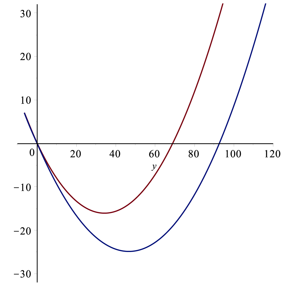
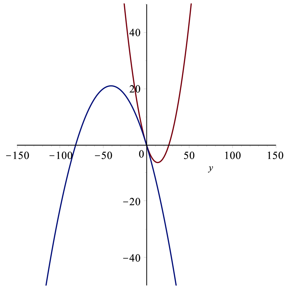
We are going to split the proof of Theorem 11 into several lemmas. Our strategy is to show that for every t∈(0,1)t\in(0,1), Δ−​(y0,y1,t)\Delta^{-}(y_{0},y_{1},t) has at least two distinct real zeros (resp. Δ+​(y0,y1,t)\Delta^{+}(y_{0},y_{1},t) has at least two nonzero distinct real zeros), see Lemmas 13 and 14, and that the four zeros obtained in this way are all distinct, see Lemma 15. Figure 3 represents an example of plot of Δ−​(y,1,t)\Delta^{-}(y,1,t) and Δ+​(y,1,t)\Delta^{+}(y,1,t), illustrating the preceding properties.

Lemma 13.

Assume that the walk is not in a configuration described in Lemma 8. For all t∈(0,1)t\in(0,1), the factor Δ+​(y,1,t)\Delta^{+}(y,1,t) has one zero in (0,1)(0,1) and one zero in (1,+∞)(1,+\infty), see Figure 3.

Proof.

Let us first remark that both B~1​(y,1)\widetilde{B}_{1}(y,1) and B~−1​(y,1)\widetilde{B}_{-1}(y,1) are nonnegative for y∈[0,+∞){y\in[0,+\infty)}, which by (16) implies that Δ+​(y,1,t)\Delta^{+}(y,1,t) and Δ−​(y,1,t)\Delta^{-}(y,1,t) are real valued on [0,+∞)[0,+\infty). We shall now prove the following: for every t∈(0,1){t\in(0,1)}, there exists εt∈(0,1)\varepsilon_{t}\in(0,1) such that

(17) Δ+​(εt,1,t)\displaystyle\Delta^{+}(\varepsilon_{t},1,t) >0,\displaystyle>0,
(18) Δ+​(1,1,t)\displaystyle\Delta^{+}(1,1,t) <0,\displaystyle<0,
(19) limy→+∞Δ+​(y,1,t)\displaystyle\lim_{y\to+\infty}\Delta^{+}(y,1,t) =+∞.\displaystyle=+\infty.

Applying the mean value theorem to Δ+​(y,1,t)\Delta^{+}(y,1,t) on [εt,+∞)[\varepsilon_{t},+\infty) readily leads to Lemma 13. It thus remains to prove (17), (18) and (19).

The inequality (17) is straightforward when Δ+​(0,1,t)=t⁡(d0,−1+2​d−1,−1​d1,−1)>0\Delta^{+}(0,1,t)=t(d_{0,-1}+2\sqrt{d_{-1,-1}d_{1,-1}})>0, since the function y↦Δ+​(y,1,t)y\mapsto\Delta^{+}(y,1,t) is continuous.

Assume now that Δ+​(0,1,t)=0{\Delta^{+}(0,1,t)=0}, in other words, that 00 is a zero of Δ+​(y,1,t)\Delta^{+}(y,1,t). In this situation, we shall prove the existence of another zero in (0,1)(0,1). We have d0,−1+2​d−1,−1​d1,−1=0{d_{0,-1}+2\sqrt{d_{-1,-1}d_{1,-1}}=0}, which implies d0,−1=d−1,−1​d1,−1=0d_{0,-1}=d_{-1,-1}d_{1,-1}=0. Assume that d−1,−1=0d_{-1,-1}=0. Then d−1,0d_{-1,0} and d1,−1d_{1,-1} are both nonzero since otherwise the walk would be in a configuration described in Lemma 8. Then by (15) and (16), Δ+​(y,1,t)\Delta^{+}(y,1,t) is equivalent at y=0y=0 to 2​t​d−1,0​d1,−1×y2t\sqrt{d_{-1,0}d_{1,-1}}\times\sqrt{y} with 2​t​d−1,0​d1,−1>02t\sqrt{d_{-1,0}d_{1,-1}}>0. For every t∈(0,1)t\in(0,1), there necessarily exists εt∈(0,1)\varepsilon_{t}\in(0,1) such that y↦Δ+​(y,1,t)y\mapsto\Delta^{+}(y,1,t) is strictly increasing in [0,εt)[0,\varepsilon_{t}). So Δ+​(εt,1,t)>0\Delta^{+}(\varepsilon_{t},1,t)>0, thereby proving (17). The case d1,−1=0d_{1,-1}=0 is similar.

To prove (18) we use the basic inequality of arithmetic and geometric means

B~1​B~−1⩽B~1+B~−12,\sqrt{\widetilde{B}_{1}\,\widetilde{B}_{-1}}\leqslant\frac{\widetilde{B}_{1}+\widetilde{B}_{-1}}{2},

which eventually entails that

Δ+​(1,1,t)=t​𝐁0​(1,1,t)+2​t​B~1​(1,1)​B~−1​(1,1)⩽t​∑di,j−1<0.\Delta^{+}(1,1,t)=t\mathbf{B}_{0}(1,1,t)+2t\sqrt{\widetilde{B}_{1}(1,1)\,\widetilde{B}_{-1}(1,1)}\leqslant t\sum d_{i,j}-1<0.

Finally we prove our claim (19). It is obvious when d0,1+2​d−1,1​d1,1>0d_{0,1}+2\sqrt{d_{-1,1}d_{1,1}}>0, as in this case Δ+​(y,1,t)\Delta^{+}(y,1,t) is equivalent when y→+∞y\to+\infty to t⁡(d0,1+2​d−1,1​d1,1)​y2t(d_{0,1}+2\sqrt{d_{-1,1}d_{1,1}})y^{2}. Since d0,1+2​d−1,1​d1,1d_{0,1}+2\sqrt{d_{-1,1}d_{1,1}} is nonnegative, the only nontrivial case is when the latter coefficient is zero. We must have d0,1=d−1,1​d1,1=0d_{0,1}=d_{-1,1}d_{1,1}=0. If d1,1=0d_{1,1}=0 then d−1,1d_{-1,1} and d1,0d_{1,0} are both nonzero, since otherwise the walk would be in one of the configurations of Lemma 8. Then B~1​(y,1)​B~−1​(y,1)\widetilde{B}_{1}(y,1)\widetilde{B}_{-1}(y,1) has degree three with positive dominant term d−1,1​d1,0d_{-1,1}d_{1,0}, while 𝐁0​(y,1,t)\mathbf{B}_{0}(y,1,t) has degree one, and therefore (19) holds. The case d−1,1=0d_{-1,1}=0 may be treated similarly. ∎

Refer to caption
Refer to caption
Figure 3. Left: plots of Δ−​(y,1,t)\Delta^{-}(y,1,t) (color red) and Δ+​(y,1,t)\Delta^{+}(y,1,t) (color blue) in the case β4>0\beta_{4}>0. Right: same plots in the case β4<0\beta_{4}<0. In all cases, the functions admit one zero in (−1,1)(-1,1) and one zero in |y|>1|y|>1
Lemma 14.

Assume that the walk is not in a configuration described in Lemma 8. For all t∈(0,1)t\in(0,1), the factor Δ−​(y,1,t)\Delta^{-}(y,1,t) has one zero in (−1,1)(-1,1). Furthermore,

  • •

    If β4>0\beta_{4}>0, Δ−​(y,1,t)\Delta^{-}(y,1,t) has one zero in (1,+∞)(1,+\infty);

  • •

    If β4=0\beta_{4}=0, [:0][1\!:\!0] is a zero of Δ−​(y0,y1,t)\Delta^{-}(y_{0},y_{1},t);

  • •

    If β4<0\beta_{4}<0, Δ−​(y,1,t)\Delta^{-}(y,1,t) has one zero in (−∞,−1)(-\infty,-1), see Figure 3.

Proof.

Though similar to that of Lemma 13, the proof is more subtle for two reasons: first, different cases may occur according to the sign of β4\beta_{4}; second, the function Δ−\Delta^{-} is not necessarily real on (−∞,0)(-\infty,0) and so one cannot directly apply the mean value theorem, as soon as negative values of yy are concerned.

Let us first consider the zero in (−1,1)(-1,1). There are two cases, according to whether the condition below is satisfied or not:

(20) ∃z∈(−1,0] such that B~1(z,1)B~−1(z,1)=0.\exists z\in(-1,0]\text{ such that }\widetilde{B}_{1}(z,1)\widetilde{B}_{-1}(z,1)=0.

We first assume that (20) is not satisfied. Remind that B~1\widetilde{B}_{1} and B~−1\widetilde{B}_{-1} are positive on [0,1][0,1]. Then they are positive on [−1,1][-1,1], and Δ−\Delta^{-} is well defined and real on [−1,1][-1,1]. Let us prove the identities

(21) Δ−​(−1,1,t)\displaystyle\Delta^{-}(-1,1,t) >0,\displaystyle>0,
(22) Δ−​(1,1,t)\displaystyle\Delta^{-}(1,1,t) <0.\displaystyle<0.

The inequality of arithmetic and geometric means gives −B~1​B~−1⩾−B~1+B~−12-\sqrt{\widetilde{B}_{1}\,\widetilde{B}_{-1}}\geqslant-\frac{\widetilde{B}_{1}+\widetilde{B}_{-1}}{2}, and finally entails that

Δ−​(−1,1,t)=t​𝐁0​(−1,1,t)−2​t​B~1​(−1,1)​B~−1​(−1,1)⩾1−t​∑i,jdi,j>0,\Delta^{-}(-1,1,t)=t\mathbf{B}_{0}(-1,1,t)-2t\sqrt{\widetilde{B}_{1}(-1,1)\,\widetilde{B}_{-1}(-1,1)}\geqslant 1-t\sum_{i,j}d_{i,j}>0,

thereby proving (21). On the other hand, B~1​(1,1)\widetilde{B}_{1}(1,1) and B~−1​(1,1)\widetilde{B}_{-1}(1,1) are both positive and with (18),

Δ−​(1,1,t)⩽Δ+​(1,1,t)<0,\Delta^{-}(1,1,t)\leqslant\Delta^{+}(1,1,t)<0,

which shows (22). Then the mean value theorem easily implies that Δ−​(y,1,t)\Delta^{-}(y,1,t) has one zero in (−1,1)(-1,1).

Assuming now that the condition (20) is satisfied, let us consider the associated zz with biggest value, i.e., with smallest absolute value. The inequality (21) might not be true anymore (simply because Δ−​(−1,1,t)\Delta^{-}(-1,1,t) might be nonreal). Instead let us prove that

(23) Δ−​(z,1,t)⩾0.\Delta^{-}(z,1,t)\geqslant 0.

Along the proof of Lemma 4, we have seen that 𝐁0​(y,1,t)\mathbf{B}_{0}(y,1,t) has no root in (−∞,0)(-\infty,0) and so has constant sign on this interval. If d0,1≠0d_{0,1}\neq 0, then the quadratic polynomial 𝐁0​(y,1,t)\mathbf{B}_{0}(y,1,t) has dominant term d0,1>0d_{0,1}>0 and is therefore positive on (−∞,0)(-\infty,0). If d0,1=0d_{0,1}=0, then the affine function 𝐁0​(y,1,t)\mathbf{B}_{0}(y,1,t) has dominant term d0,0−1/t<0d_{0,0}-1/t<0 (we use t∈(0,1)t\in(0,1) and d0,0∈[0,1]d_{0,0}\in[0,1]) and is also positive on (−∞,0)(-\infty,0). Therefore 𝐁0​(z,1,t)⩾0\mathbf{B}_{0}(z,1,t)\geqslant 0. With B~1​(z,1)​B~−1​(z,1)=0\widetilde{B}_{1}(z,1)\widetilde{B}_{-1}(z,1)=0, we deduce (23). Note that (22) still holds true in this context. By construction, B~1​(z,1)​B~−1​(z,1)⩾0\widetilde{B}_{1}(z,1)\widetilde{B}_{-1}(z,1)\geqslant 0 on [z,0]⊂[z,1][z,0]\subset[z,1]. Applying the mean value theorem we deduce that Δ−​(y,1,t)\Delta^{-}(y,1,t) has one zero in [z,1)⊂(−1,1)[z,1)\subset(-1,1).

We now focus on the other zero of Δ−\Delta^{-}. Consider first the subcase β4>0\beta_{4}>0. Recall that by (14) the condition β4>0\beta_{4}>0 is equivalent to d0,1>2​d1,1​d−1,1d_{0,1}>2\sqrt{d_{1,1}d_{-1,1}}. Therefore one obtains

(24) limy→+∞Δ−​(y,1,t)=+∞if ​β4>0.\lim_{y\to+\infty}\Delta^{-}(y,1,t)=+\infty\quad\text{if }\beta_{4}>0.

Together with (22), the mean value theorem implies that for β4>0\beta_{4}>0, Δ−​(y,1,t)\Delta^{-}(y,1,t) has at least one real zero in (1,+∞)(1,+\infty).

If β4=0\beta_{4}=0, [:0][1\!:\!0] is obviously a zero of Δ−​(y0,y1,t)\Delta^{-}(y_{0},y_{1},t). If now β4<0\beta_{4}<0, i.e.,

(25) 0⩽d0,1<2​d1,1​d−1,1,0\leqslant d_{0,1}<2\sqrt{d_{1,1}d_{-1,1}},

then we must have d1,1​d−1,1≠0d_{1,1}d_{-1,1}\neq 0, for otherwise (25) could not be true. Then both B~1​(y,1)\widetilde{B}_{1}(y,1) and B~−1​(y,1)\widetilde{B}_{-1}(y,1) have degree two with a positive dominant term. Therefore

limy→−∞B~1​(y,1)​B~−1​(y,1)=+∞.\lim_{y\to-\infty}\widetilde{B}_{1}(y,1)\widetilde{B}_{-1}(y,1)=+\infty.

Consider now the condition

(26) ∃z⩽0​ such that ​B~1​(z,1)​B~−1​(z,1)=0.\exists z\leqslant 0\text{ such that }\widetilde{B}_{1}(z,1)\widetilde{B}_{-1}(z,1)=0.

Remind that B~1​(y,1)​B~−1​(y,1)\widetilde{B}_{1}(y,1)\widetilde{B}_{-1}(y,1) is strictly positive on (0,+∞)(0,+\infty). If there is no zz satisfying to (26), then Δ−\Delta^{-} is real on ℝ\mathbb{R}, and using (25) we easily compute

(27) limy→−∞Δ−​(y,1,t)=−∞if ​β4<0.\lim_{y\to-\infty}\Delta^{-}(y,1,t)=-\infty\quad\text{if }\beta_{4}<0.

We conclude by the mean value theorem applied to the function Δ−\Delta^{-} on (−∞,−1)(-\infty,-1), using further (21).

If (26) holds true, let us consider the smallest zz, i.e., with largest absolute value. Then (23) is satisfied and we conclude by the same line of argument. The proof is complete. ∎

Lemma 15.

Assume that the walk is not in a configuration described in Lemma 8. For all t∈(0,1){t\in(0,1)} and [y0:y1]∈ℙ1(ℂ)∖{[:1]}[y_{0}\!:\!y_{1}]\in\mathbb{P}^{1}(\mathbb{C})\setminus\{[0\!:\!1]\} such that Δ+​(y0,y1,t)=0\Delta^{+}(y_{0},y_{1},t)=0,

(28) Δ−​(y0,y1,t)≠Δ+​(y0,y1,t).\Delta^{-}(y_{0},y_{1},t)\neq\Delta^{+}(y_{0},y_{1},t).
Proof.

Thanks to (19), [:0][1\!:\!0] cannot be a zero of the factor Δ+​(y0,y1,t)\Delta^{+}(y_{0},y_{1},t). So we may assume that [y0:y1]=[y:1][y_{0}\!:\!y_{1}]=[y\!:\!1] with y∈ℂ∗y\in\mathbb{C}^{*}. If Δ−​(y,1,t)=Δ+​(y,1,t)\Delta^{-}(y,1,t)=\Delta^{+}(y,1,t) for some tt, then necessarily

(29) 𝐁0​(y,1,t)=B~1​(y,1)=0or𝐁0​(y,1,t)=B~−1​(y,1)=0.\mathbf{B}_{0}(y,1,t)=\widetilde{B}_{1}(y,1)=0\quad\text{or}\quad\mathbf{B}_{0}(y,1,t)=\widetilde{B}_{-1}(y,1)=0.

Lemma 4 yields y=0y=0. Thus for t∈(0,1)t\in(0,1), [y0:y1]∈ℙ1(ℂ)∖{[:1]}[y_{0}\!:\!y_{1}]\in\mathbb{P}^{1}(\mathbb{C})\setminus\{[0\!:\!1]\}, with Δ+​(y0,y1,t)=0{\Delta^{+}(y_{0},y_{1},t)=0}, we have Δ−​(y0,y1,t)≠Δ+​(y0,y1,t)\Delta^{-}(y_{0},y_{1},t)\neq\Delta^{+}(y_{0},y_{1},t). ∎

We are now able to show Theorem 11.

Proof of Theorem 11.

By Lemmas 13 and 14, Δ−​(y0,y1,t)\Delta^{-}(y_{0},y_{1},t) has at least two distinct real zeros (resp. Δ+​(y0,y1,t)\Delta^{+}(y_{0},y_{1},t) has at least two distinct nonzero real zeros). With Lemma 15, the four zeros are distinct. Going back to Lemmas 13 and 14, we obtain that they are located as stated in Theorem 11. ∎

Remark 16.

If the weights are not supported in any half-space (or equivalently, if the steps are not in a configuration of Lemma 8), then the step set polynomial S⁡(x,y)=∑di,j​xi​yjS(x,y)=\sum d_{i,j}x^{i}y^{j} defined in (4) has a unique global minimizing point (x0,y0)(x_{0},y_{0}) on ℝ>02\mathbb{R}_{>0}^{2}, which satisfies

∂S∂x​(x0,y0)=∂S∂y​(x0,y0)=0,\frac{\partial S}{\partial x}(x_{0},y_{0})=\frac{\partial S}{\partial y}(x_{0},y_{0})=0,

see [BRS14, Theorem 4]. (This point (x0,y0)(x_{0},y_{0}) is important, in particular S⁡(x0,y0)S(x_{0},y_{0}) is related to the exponential growth of the total number of excursions by [BRS14, Theorem 4].) Obviously one has S⁡(x0,y0)⩽S⁡(1,1)=1S(x_{0},y_{0})\leqslant S(1,1)=1, as (x0,y0)(x_{0},y_{0}) is a global minimizer. Taking

t=t0=1S⁡(x0,y0)⩾1,t=t_{0}=\frac{1}{S(x_{0},y_{0})}\geqslant 1,

the point (x0,y0)(x_{0},y_{0}) is a singularity of E¯t\overline{E}_{t} (for t=t0t=t_{0}), and E¯t\overline{E}_{t} becomes of genus 00, see Proposition 7.

We conjecture that t0t_{0} is the smallest value of t>0t>0 for which E¯t\overline{E}_{t} has genus 00. This holds true in case of a zero drift, for which t0=1t_{0}=1 and two branch points are equal to 11 by [FIM99, Chapter 6].

Assumption 17.

From now we assume that the model is nondegenerate and that E¯t\overline{E}_{t} is an elliptic curve.

Recall that Proposition 9 gives a very simple characterization of walks satisfying Assumption 17.

1.5. Group of the walk

Following [FIM99, Chapter 2], [BMM10, Section 3] or [KY15, Section 3], we attach to any model its group, which by definition is the group ⟨i1,i2⟩\langle i_{1},i_{2}\rangle generated by the involutive birational transformations of ℙ1​(ℂ)2\mathbb{P}^{1}(\mathbb{C})^{2} given by

(30) ι1​(x,y)=(x0x1,A−1​(x0x1)A1​(x0x1)​y0y1)andι2​(x,y)=(B−1​(y0y1)B1​(y0y1)​x0x1,y0y1),\iota_{1}(x,y)=\left(\frac{x_{0}}{x_{1}},\frac{A_{-1}(\frac{x_{0}}{x_{1}})}{A_{1}(\frac{x_{0}}{x_{1}})\frac{y_{0}}{y_{1}}}\right)\quad\text{and}\quad\iota_{2}(x,y)=\left(\frac{B_{-1}(\frac{y_{0}}{y_{1}})}{B_{1}(\frac{y_{0}}{y_{1}})\frac{x_{0}}{x_{1}}},\frac{y_{0}}{y_{1}}\right),

with our notation (4).

Refer to caption
Figure 4. The maps ι1\iota_{1} and ι2\iota_{2} restricted to the kernel curve E¯t\overline{E}_{t}

The kernel curve E¯t\overline{E}_{t} is left invariant by the natural action of this group, see (8). For a fixed value of xx, there are at most two possible values of yy such that (x,y)∈E¯t(x,y)\in\overline{E}_{t}. The involution ι1\iota_{1} corresponds to interchanging these values, see Figure 4. A similar interpretation can be given for ι2\iota_{2}.

Let us finally define

τ=ι2∘ι1.\tau=\iota_{2}\circ\iota_{1}.

Note that such a map is known as a QRT-map and has been widely studied, see [Dui10]. As we will see later, the algebraic nature of the series (2), according to the classes depicted in (3), highly depends on the fact that τ\tau has finite or infinite order. Note that when the di,jd_{i,j} are fixed, the cardinality of the group on E¯t\overline{E}_{t} depends upon tt, see [FR11] for concrete examples.

2. Analytic continuation of the generating functions

The goal of this section is to prove that F1​(x,t)F^{1}(x;t) and F2​(y,t)F^{2}(y;t) defined in (6) may be continued into multivalued meromorphic functions on the elliptic curve E¯t\overline{E}_{t}. We are going to use a uniformization of E¯t\overline{E}_{t} via the Weierstrass elliptic function in order to see the multivalued functions as univalued meromorphic functions on ℂ\mathbb{C}. The starting point is that for tt fixed in (0,1)(0,1), the generating function Q⁡(x,y,t)Q(x,y;t) is analytic for |x|,|y|<1|x|,|y|<1, see Section 1.

2.1. Uniformization of the elliptic curve E¯t\overline{E}_{t}

Recall that Assumption 17 holds: the walk is nondegenerate and E¯t\overline{E}_{t} is an elliptic curve. This implies (Proposition 7) that the discriminants Δx[x0:x1]\Delta^{x}_{[x_{0}:x_{1}]} and Δy[y0:y1]\Delta^{y}_{[y_{0}:y_{1}]} have four distinct zeros.

Since E¯t\overline{E}_{t} is an elliptic curve, we can identify E¯t\overline{E}_{t} with ℂ/(ℤ​ω1+ℤ​ω2)\mathbb{C}/(\mathbb{Z}\omega_{1}+\mathbb{Z}\omega_{2}), with (ω1,ω2)∈ℂ2(\omega_{1},\omega_{2})\in\mathbb{C}^{2} basis of a lattice, via the (ℤ​ω1+ℤ​ω2)(\mathbb{Z}\omega_{1}+\mathbb{Z}\omega_{2})-periodic map

(31) Λ:ℂ→E¯tω↦(𝔮1​(ω),𝔮2​(ω)),\begin{array}[]{llll}\Lambda:&\mathbb{C}&\rightarrow&\overline{E}_{t}\\ &\omega&\mapsto&(\mathfrak{q}_{1}(\omega),\mathfrak{q}_{2}(\omega)),\end{array}

where 𝔮1,𝔮2\mathfrak{q}_{1},\mathfrak{q}_{2} are rational functions of ℘\wp and its derivative d​℘/d​ωd\wp/d\omega, and ℘\wp is the Weierstrass function associated with the lattice ℤ​ω1+ℤ​ω2\mathbb{Z}\omega_{1}+\mathbb{Z}\omega_{2}:

(32) ℘⁡(ω)=℘⁡(ω,ω1,ω2):=1ω2+∑(ℓ1,ℓ2)∈ℤ2∖{(0,0)}(1(ω+ℓ1​ω1+ℓ2​ω2)2−1(ℓ1​ω1+ℓ2​ω2)2).\wp(\omega)=\wp(\omega;\omega_{1},\omega_{2}):=\frac{1}{\omega^{2}}+\sum_{(\ell_{1},\ell_{2})\in\mathbb{Z}^{2}\setminus\{(0,0)\}}\left(\frac{1}{(\omega+\ell_{1}\omega_{1}+\ell_{2}\omega_{2})^{2}}-\frac{1}{(\ell_{1}\omega_{1}+\ell_{2}\omega_{2})^{2}}\right).

Then the field of meromorphic functions on E¯t\overline{E}_{t} may be identified with the field of meromorphic functions on ℂ/(ℤ​ω1+ℤ​ω2)\mathbb{C}/(\mathbb{Z}\omega_{1}+\mathbb{Z}\omega_{2}), i.e., the field of meromorphic functions on ℂ\mathbb{C} that are (ω1,ω2)(\omega_{1},\omega_{2})-periodic (or elliptic). Classically, this latter field is equal to ℂ⁡(℘,℘′)\mathbb{C}(\wp,\wp^{\prime}), see [WW96].

The goal of this subsection is to give explicit expressions for 𝔮1​(ω)\mathfrak{q}_{1}(\omega), 𝔮2​(ω)\mathfrak{q}_{2}(\omega), ω1\omega_{1} and ω2\omega_{2}. Such computations have been already performed in [FIM99, Section 3.3] when t=1t=1, and in [Ras12] in the unweighted case for t∈(0,1/|𝒮|)t\in(0,1/|\mathcal{S}|).

The maps ι1\iota_{1}, ι2\iota_{2} and τ\tau may be lifted to the ω\omega-plane. We will call them ι~1{\widetilde{\iota}}_{1}, ι~2{\widetilde{\iota}}_{2} and τ~\widetilde{\tau}, respectively. So we have the commutative diagrams

E¯t\textstyle{\overline{E}_{t}\ignorespaces\ignorespaces\ignorespaces\ignorespaces}ιk\scriptstyle{\iota_{k}}E¯t\textstyle{\overline{E}_{t}}ℂ\textstyle{\mathbb{C}\ignorespaces\ignorespaces\ignorespaces\ignorespaces\ignorespaces\ignorespaces\ignorespaces\ignorespaces}Λ\scriptstyle{\Lambda}ι~k\scriptstyle{{\widetilde{\iota}}_{k}}ℂ\textstyle{\mathbb{C}\ignorespaces\ignorespaces\ignorespaces\ignorespaces}Λ\scriptstyle{\Lambda}      E¯t\textstyle{\overline{E}_{t}\ignorespaces\ignorespaces\ignorespaces\ignorespaces}τ\scriptstyle{\tau}E¯t\textstyle{\overline{E}_{t}}ℂ\textstyle{\mathbb{C}\ignorespaces\ignorespaces\ignorespaces\ignorespaces\ignorespaces\ignorespaces\ignorespaces\ignorespaces}Λ\scriptstyle{\Lambda}τ~\scriptstyle{\widetilde{\tau}}ℂ\textstyle{\mathbb{C}\ignorespaces\ignorespaces\ignorespaces\ignorespaces}Λ\scriptstyle{\Lambda}

More precisely, following [Dui10] (see in particular Proposition 2.5.2, Page 35 and Remark 2.3.8), there exist two complex numbers ω3\omega_{3} and ω4\omega_{4} such that

(33) ι~1(ω)=−ω+ω4,ι~2(ω)=−ω+ω3andτ~(ω)=ω−ω4+ω3.{\widetilde{\iota}}_{1}(\omega)=-\omega+\omega_{4},\quad{\widetilde{\iota}}_{2}(\omega)=-\omega+\omega_{3}\quad\text{and}\quad\widetilde{\tau}(\omega)=\omega-\omega_{4}+\omega_{3}.

Up to a variable change of the form ω↦ω+ω4\omega\mapsto\omega+\omega_{4}, we may always reduce to the case ω4=0\omega_{4}=0. So let us assume that ω4=0\omega_{4}=0 in (33).

We have Λ⁡(ω)=Λ⁡(ω+ω1)=Λ⁡(ω+ω2)\Lambda(\omega)=\Lambda(\omega+\omega_{1})=\Lambda(\omega+\omega_{2}) for all ω∈ℂ\omega\in\mathbb{C}. This implies that for all ℓ1,ℓ2∈ℤ\ell_{1},\ell_{2}\in\mathbb{Z}, ι~2{\widetilde{\iota}}_{2} may be replaced by ω↦−ω+ω3+ℓ1​ω1+ℓ2​ω2\omega\mapsto-\omega+\omega_{3}+\ell_{1}\omega_{1}+\ell_{2}\omega_{2}. This shows that ω3\omega_{3} is not uniquely defined: it is only defined modulo the lattice ℤ​ω1+ℤ​ω2\mathbb{Z}\omega_{1}+\mathbb{Z}\omega_{2}. A suitable choice of ω1\omega_{1}, ω2\omega_{2} and ω3\omega_{3} will be made in Proposition 18 and Lemma 23.

Using (11) and (13), the discriminant D⁡(x)D(x) can be written as

D⁡(x)=B2​(x)−4​A​(x)​C​(x),D(x)=B^{2}(x)-4A(x)C(x),

with

{A⁡(x)=t⁡(d−1,1+d0,1​x+d1,1​x2),B⁡(x)=t⁡(d−1,0−1t​x+d0,0​x+d1,0​x2),C⁡(x)=t⁡(d−1,−1+d0,−1​x+d1,−1​x2).\left\{\begin{array}[]{rl}A(x)&\hskip-8.53581pt=t(d_{-1,1}+d_{0,1}x+d_{1,1}x^{2}),\\ B(x)&\hskip-8.53581pt=t(d_{-1,0}-\frac{1}{t}x+d_{0,0}x+d_{1,0}x^{2}),\\ C(x)&\hskip-8.53581pt=t(d_{-1,-1}+d_{0,-1}x+d_{1,-1}x^{2}).\end{array}\right.

The link between the above notations and the A~i\widetilde{A}_{i}’s used in Section 1 is A=t​A~1A=t\widetilde{A}_{1}, B=t​A~0−xB=t\widetilde{A}_{0}-x and C=t​A~−1C=t\widetilde{A}_{-1}.

The following proposition is the adaptation of [FIM99, Lemma 3.3.1] to our context. Remind that we have ordered the aia_{i}’s in such a way that the cycle of ℙ1​(ℝ)\mathbb{P}^{1}(\mathbb{R}) starting from −1-1 and going to +∞+\infty, and then from −∞-\infty to −1-1, crosses the aia_{i}’s in the order a1,a2,a3,a4a_{1},a_{2},a_{3},a_{4}, see Figure 2 and Remark 12. Before stating Proposition 18, note the following convention: a path of integration in an integral of the form ∫aiaj\int_{a_{i}}^{a_{j}} is the real path from aia_{i} to aja_{j} if ai⩽aja_{i}\leqslant a_{j}, and otherwise is the union of the real paths from aia_{i} to +∞+\infty and from −∞-\infty to aja_{j}.

Proposition 18.

The elliptic curve E¯t\overline{E}_{t} in (8) admits a uniformization of the form

E¯t={(x⁡(ω),y⁡(ω)):ω∈ℂ/(ℤ​ω1+ℤ​ω2)},\overline{E}_{t}=\bigl\{(x(\omega),y(\omega)):\omega\in\mathbb{C}/(\mathbb{Z}\omega_{1}+\mathbb{Z}\omega_{2})\bigr\},

where x⁡(ω)x(\omega) and y⁡(ω)y(\omega) are given by (note that z=2​A​(x)​y+B⁡(x)z=2A(x)y+B(x))

x⁡(ω)z⁡(ω)a4≠[:0][a4+D′​(a4)℘⁡(ω)−16​D′′​(a4):1][D′​(a4)​℘′​(ω)2​(℘⁡(ω)−16​D′′​(a4))2:1]a4=[:0][℘(ω)−α2/3:α3][−℘′(ω):2α3]\begin{array}[]{|l|c|c|}\hline\cr&x(\omega)&z(\omega)\\ \hline\cr a_{4}\neq[1\!:\!0]&\phantom{\Bigg\|}\left[a_{4}+\frac{D^{\prime}(a_{4})}{\wp(\omega)-\frac{1}{6}D^{\prime\prime}(a_{4})}:1\right]&\phantom{\Bigg\|}\left[\frac{D^{\prime}(a_{4})\wp^{\prime}(\omega)}{2(\wp(\omega)-\frac{1}{6}D^{\prime\prime}(a_{4}))^{2}}:1\right]\\ \hline\cr a_{4}=[1\!:\!0]&\phantom{\Big\|}\left[\wp(\omega)-\alpha_{2}/3:\alpha_{3}\right]&\phantom{\Big\|}\left[-\wp^{\prime}(\omega):2\alpha_{3}\right]\\ \hline\cr\end{array}

The above formulas use the Weierstrass elliptic function ℘⁡(ω)=℘⁡(ω,ω1,ω2)\wp(\omega)=\wp(\omega;\omega_{1},\omega_{2}) defined in (32). Moreover, a suitable choice for the periods (ω1,ω2)(\omega_{1},\omega_{2}) is given by the elliptic integrals

(34) ω1=𝐢​∫a3a4d​x|D⁡(x)|∈𝐢​ℝ>0andω2=∫a4a1d​xD⁡(x)∈ℝ>0.\omega_{1}=\mathbf{i}\int_{a_{3}}^{a_{4}}\frac{dx}{\sqrt{|D(x)|}}\in\mathbf{i}\mathbb{R}_{>0}\quad\text{and}\quad\omega_{2}=\int_{a_{4}}^{a_{1}}\frac{dx}{\sqrt{D(x)}}\in\mathbb{R}_{>0}.

Before proving Proposition 18, let us do a series of remarks.

∙\bullet Formula (34) is stated in [FIM99, Lemma 3.3.2] for t=1t=1. Note a small misprint in [FIM99, Lemma 3.3.2], namely a (multiplicative) factor of 22 that should be 11.

∙\bullet Note that the expression (34) for the periods is not unique (however, it is unique up to a unimodular transform). Our motivation for doing this particular choice is to have a real positive period (namely, ω2\omega_{2}) and a purely imaginary one (ω1\omega_{1}).

∙\bullet As we shall see along the proof, the elliptic curve E¯t\overline{E}_{t} admits the classical Weierstrass canonical form

(35) E¯t={(𝐮,v)∈ℙ1​(ℂ)2:v2=4​𝐮3−g2​𝐮−g3},\overline{E}_{t}=\{(\mathbf{u},v)\in\mathbb{P}^{1}(\mathbb{C})^{2}:v^{2}=4\mathbf{u}^{3}-g_{2}\mathbf{u}-g_{3}\},

with real invariants g2,g3g_{2},g_{3} defined in (38) (resp. (37)) in the case a4≠[:0]a_{4}\neq[1\!:\!0] (resp. a4=[:0]a_{4}=[1\!:\!0]). Furthermore, the discriminant of 4​𝐮3−g2​𝐮−g34\mathbf{u}^{3}-g_{2}\mathbf{u}-g_{3} is positive.

∙\bullet Obviously, replacing zz by −z-z in the statement of Proposition 18 gives another equivalent uniformization, see (36). We have arbitrarily fixed the sign of zz by demanding that zz and ℘′\wp^{\prime} should have the same sign, as in [FIM99, Lemma 3.3.1].

∙\bullet An alternative, more symmetric formula for the second coordinate of the uniformization y⁡(ω)y(\omega) will be given in (46).

∙\bullet Remind that ω3\omega_{3} is defined modulo the lattice. In what follows, with the above expressions (34) of ω1\omega_{1} and ω2\omega_{2}, we will fix ω3\omega_{3} in the fundamental parallelogram [0,ω1)+[0,ω2)[0,\omega_{1})+[0,\omega_{2}). Remark that an explicit formula for ω3\omega_{3} will be obtained in (47).

Proof of Proposition 18.

Letting z=2​A​(x)​y+B⁡(x)z=2A(x)y+B(x), the equality K¯​(x,y,t)=0\overline{K}(x,y;t)=0 can easily be reformulated as

(36) z2=D⁡(x).z^{2}=D(x).

Assume first that a4=[:0]a_{4}=[1\!:\!0]. We have α4=0\alpha_{4}=0 in (13) and thus α3≠0\alpha_{3}\neq 0 (otherwise [:0][1\!:\!0] would be a double zero of the discriminant, contradicting our assumption). In this case we perform the changes of variable

x=𝐮−α2/3α3andz=−v2​α3x=\frac{\mathbf{u}-\alpha_{2}/3}{\alpha_{3}}\quad\text{and}\quad z=\frac{-v}{2\alpha_{3}}

in order to recover the Weierstrass canonical form (35). We just have to set 𝐮=℘\mathbf{u}=\wp and v=℘′v=\wp^{\prime} to obtain the result announced in Proposition 18. In this case the invariants are given by

(37) g2=43​α22−4​α1​α3andg3=−827​α23+43​α1​α2​α3−4​α0​α32.g_{2}=\frac{4}{3}\alpha_{2}^{2}-4\alpha_{1}\alpha_{3}\quad\text{and}\quad g_{3}=-\frac{8}{27}\alpha_{2}^{3}+\frac{4}{3}\alpha_{1}\alpha_{2}\alpha_{3}-4\alpha_{0}\alpha_{3}^{2}.

In particular, g2g_{2} and g3g_{3} are clearly polynomial functions of tt.

Assume now that a4≠[:0]a_{4}\neq[1\!:\!0]. The main idea is to reduce to the case a4=[:0]a_{4}=[1\!:\!0] by performing a fractional linear transformation. The branch point a4a_{4} is a simple zero of D⁡(x)D(x) and hence D′​(a4)≠0D^{\prime}(a_{4})\neq 0. Introduce

u=D′​(a4)x−a4andv=2​z​D′​(a4)(x−a4)2.u=\frac{D^{\prime}(a_{4})}{x-a_{4}}\quad\text{and}\quad v=\frac{2zD^{\prime}(a_{4})}{(x-a_{4})^{2}}.

Then the Taylor formula D⁡(x)=∑j=14(x−a4)j​D(j)​(a4)j!D(x)=\sum_{j=1}^{4}(x-a_{4})^{j}\frac{D^{(j)}(a_{4})}{j!} allows us to express (36) as

v2=4​u3+2​D′′​(a4)​u2+2​u3​D(3)​(a4)​D′​(a4)+D(4)​(a4)​D′​(a4)26.v^{2}=4u^{3}+2D^{\prime\prime}(a_{4})u^{2}+\frac{2u}{3}D^{(3)}(a_{4})D^{\prime}(a_{4})+\frac{D^{(4)}(a_{4})D^{\prime}(a_{4})^{2}}{6}.

Letting finally 𝐮=u+D′′​(a4)6\mathbf{u}=u+\frac{D^{\prime\prime}(a_{4})}{6}, we obtain the Weierstrass canonical form (35), where

(38) g2=D′′​(a4)23−2​D′​(a4)​D(3)​(a4)3andg3=−D′′​(a4)327+D′​(a4)​D′′​(a4)​D(3)​(a4)9−D′​(a4)2​D(4)​(a4)6.g_{2}=\frac{D^{\prime\prime}(a_{4})^{2}}{3}-\frac{2D^{\prime}(a_{4})D^{(3)}(a_{4})}{3}\\ \text{and}\quad g_{3}=-\frac{D^{\prime\prime}(a_{4})^{3}}{27}+\frac{D^{\prime}(a_{4})D^{\prime\prime}(a_{4})D^{(3)}(a_{4})}{9}-\frac{D^{\prime}(a_{4})^{2}D^{(4)}(a_{4})}{6}.

Again, we just have to set 𝐮=℘\mathbf{u}=\wp and v=℘′v=\wp^{\prime} to obtain the result.

In both cases the invariants g2,g3g_{2},g_{3} are real and the discriminant of 4​𝐮3−g2​𝐮−g34\mathbf{u}^{3}-g_{2}\mathbf{u}-g_{3} is strictly positive (this follows from the fact that the aia_{i}’s are real and distinct). Let e1>e2>e3e_{1}>e_{2}>e_{3} be the three real roots of the discriminant. By [WW96, Section 20.32, Example 1] we may choose ω1,ω2\omega_{1},\omega_{2} as follows (here we replace ω1\omega_{1} by −ω1-\omega_{1} in order to have a period in 𝐢​ℝ>0\mathbf{i}\mathbb{R}_{>0}):

(39) ω1=2​𝐢​∫−∞e3d​𝐮g2​𝐮+g3−4​𝐮3andω2=2​∫e1+∞d​𝐮4​𝐮3−g2​𝐮−g3.\omega_{1}=2\mathbf{i}\int_{-\infty}^{e_{3}}\frac{d\mathbf{u}}{\sqrt{g_{2}\mathbf{u}+g_{3}-4\mathbf{u}^{3}}}\quad\text{and}\quad\omega_{2}=2\int_{e_{1}}^{+\infty}\frac{d\mathbf{u}}{\sqrt{4\mathbf{u}^{3}-g_{2}\mathbf{u}-g_{3}}}.

In particular ω2\omega_{2} is real while ω1\omega_{1} is a pure imaginary.

Note that since 4​𝐮3−g2​𝐮−g34\mathbf{u}^{3}-g_{2}\mathbf{u}-g_{3} has three distinct real roots, one has by [WW96, Section 20.32]

(40) e1=℘⁡(ω22)>e2=℘⁡(ω1+ω22)>e3=℘⁡(ω12).e_{1}=\wp\left(\frac{\omega_{2}}{2}\right)>e_{2}=\wp\left(\frac{\omega_{1}+\omega_{2}}{2}\right)>e_{3}=\wp\left(\frac{\omega_{1}}{2}\right).

We now prove that, with x⁡(ω)x(\omega) as in the statement of Proposition 18,

(41) x⁡(0)=a4,x⁡(ω12)=a3,x⁡(ω1+ω22)=a2,x⁡(ω22)=a1.x(0)=a_{4},\quad x\left(\frac{\omega_{1}}{2}\right)=a_{3},\quad x\left(\frac{\omega_{1}+\omega_{2}}{2}\right)=a_{2},\quad x\left(\frac{\omega_{2}}{2}\right)=a_{1}.

The correspondence in (41) is illustrated on Figure 5. Let us first note that the change of variable between the xx-variable in (36) and the 𝐮\mathbf{u}-variable in (40) is just

(42) x={a4+D′​(a4)𝐮−D′′​(a4)6when a4≠[:0],𝐮−α2/3α3otherwise.x=\left\{\begin{array}[]{ll}\displaystyle a_{4}+\frac{D^{\prime}(a_{4})}{\mathbf{u}-\frac{D^{\prime\prime}(a_{4})}{6}}&\text{when }a_{4}\neq[1\!:\!0],\\ \displaystyle\frac{\mathbf{u}-\alpha_{2}/3}{\alpha_{3}}&\text{otherwise}.\end{array}\right.

Remind that a1,a2,a3,a4a_{1},a_{2},a_{3},a_{4} are the roots of the discriminant. By construction the roots of Δx[x0:x1]\Delta^{x}_{[x_{0}:x_{1}]} correspond to the double roots of y↦K¯​(aj,y,t)y\mapsto\overline{K}(a_{j},y;t). Therefore, the (aj,Y±​(aj))(a_{j},Y_{\pm}(a_{j})) are the fixed points by ι1\iota_{1}. Since a1,a2,a3,a4a_{1},a_{2},a_{3},a_{4} are distinct and {0,ω12,ω22,ω1+ω22}\{0,\frac{\omega_{1}}{2},\frac{\omega_{2}}{2},\frac{\omega_{1}+\omega_{2}}{2}\} are the four distinct fixed points modulo ℤ​ω1+ℤ​ω2\mathbb{Z}\omega_{1}+\mathbb{Z}\omega_{2} of ι~1​(ω)=−ω{\widetilde{\iota}}_{1}(\omega)=-\omega, we find the equality of sets

Λ⁡{0,ω12,ω22,ω1+ω22}={(a1,Y±​(a1)),(a2,Y±​(a2)),(a3,Y±​(a3)),(a4,Y±​(a4))}.\Lambda\left\{0,\frac{\omega_{1}}{2},\frac{\omega_{2}}{2},\frac{\omega_{1}+\omega_{2}}{2}\right\}=\bigl\{(a_{1},Y_{\pm}(a_{1})),(a_{2},Y_{\pm}(a_{2})),(a_{3},Y_{\pm}(a_{3})),(a_{4},Y_{\pm}(a_{4}))\bigr\}.

By construction we have x⁡(0)=a4x(0)=a_{4}. To pursue, note that

α3=2​d1,0​(d0,0−1/t)−4​d1,1​d0,−1−4​d0,1​d1,−1,\alpha_{3}=2d_{1,0}(d_{0,0}-1/t)-4d_{1,1}d_{0,-1}-4d_{0,1}d_{1,-1},

see (14). Since the di,jd_{i,j}’s are positive and d0,0−1/t<0d_{0,0}-1/t<0 (we use t∈(0,1)t\in(0,1)), we obtain α3⩽0\alpha_{3}\leqslant 0.

In the case a4=[:0]a_{4}=[1\!:\!0] we must have α4=0\alpha_{4}=0 and α3≠0\alpha_{3}\neq 0. Hence α3<0\alpha_{3}<0, and the function in (42) is decreasing. With (40) we conclude that

x⁡(ω22)<x⁡(ω1+ω22)<x⁡(ω12),x\left(\frac{\omega_{2}}{2}\right)<x\left(\frac{\omega_{1}+\omega_{2}}{2}\right)<x\left(\frac{\omega_{1}}{2}\right),

and thus (41) holds since a1<a2<a3<a4=+∞a_{1}<a_{2}<a_{3}<a_{4}=+\infty, see Figure 2, Theorem 11 and Remark 12.

Let us now consider the case a4≠[:0]a_{4}\neq[1\!:\!0] and α4>0\alpha_{4}>0. With the assertion on the sign of a3,a4a_{3},a_{4} in Theorem 11, we deduce that a4a_{4} is the biggest root, see Figure 2. Hence D′​(a4)>0D^{\prime}(a_{4})>0. Since all of a1,a2,a3a_{1},a_{2},a_{3} are smaller than a4a_{4} we must have, due to (42), ei<D′′​(a4)6e_{i}<\frac{D^{\prime\prime}(a_{4})}{6}. The function (42) being decreasing for 𝐮∈(−∞,D′′​(a4)6)\mathbf{u}\in(-\infty,\frac{D^{\prime\prime}(a_{4})}{6}) and the eie_{i}’s being ordered as in (40), we deduce (41), similarly to the case a4=[:0]a_{4}=[1\!:\!0].

Consider finally the case a4≠[:0]a_{4}\neq[1\!:\!0] and α4<0\alpha_{4}<0. With the assertion on the sign of a3,a4a_{3},a_{4} in Theorem 11, we deduce that a4a_{4} is the smallest root, see Figure 2. Hence D′​(a4)>0D^{\prime}(a_{4})>0. Since all of a1,a2,a3a_{1},a_{2},a_{3} are bigger than a4a_{4} we must have, due to (42), ei>D′′​(a4)6e_{i}>\frac{D^{\prime\prime}(a_{4})}{6}. The function (42) being decreasing for 𝐮∈(D′′​(a4)6,+∞)\mathbf{u}\in(\frac{D^{\prime\prime}(a_{4})}{6},+\infty) and the eie_{i}’s being ordered as in (40), we deduce (41).

We now move to the proof of the formulas (34) for the periods. To that purpose, we perform in (39) the variable change (42). We first assume that a4≠[:0]a_{4}\neq[1\!:\!0]. A straightforward computation shows that

(43) D⁡(x)=z2=v2​(x−a4)44​D′​(a4)2=(x−a4)44​D′​(a4)2​(4​𝐮3−g2​𝐮−g3).D(x)=z^{2}=v^{2}\frac{(x-a_{4})^{4}}{4D^{\prime}(a_{4})^{2}}=\frac{(x-a_{4})^{4}}{4D^{\prime}(a_{4})^{2}}(4\mathbf{u}^{3}-g_{2}\mathbf{u}-g_{3}).

In particular 4​𝐮3−g2​𝐮−g3=2​D′​(a4)(x−a4)2​D⁡(x)\sqrt{4\mathbf{u}^{3}-g_{2}\mathbf{u}-g_{3}}=\frac{2D^{\prime}(a_{4})}{(x-a_{4})^{2}}\sqrt{D(x)}. Therefore with (39) d​𝐮=−D′​(a4)(x−a4)2​d​xd\mathbf{u}=\frac{-D^{\prime}(a_{4})}{(x-a_{4})^{2}}dx, and with (41) we find

ω2=2​∫℘⁡(ω22)+∞d​𝐮4​𝐮3−g2​𝐮−g3=∫a4a1d​xD⁡(x).\omega_{2}=2\int_{\wp(\frac{\omega_{2}}{2})}^{+\infty}\frac{d\mathbf{u}}{\sqrt{4\mathbf{u}^{3}-g_{2}\mathbf{u}-g_{3}}}=\int_{a_{4}}^{a_{1}}\frac{dx}{\sqrt{D(x)}}.

Similarly, −4​𝐮3+g2​𝐮+g3-4\mathbf{u}^{3}+g_{2}\mathbf{u}+g_{3} is positive for 𝐮∈(−∞,e3)\mathbf{u}\in(-\infty,e_{3}) and

ω1=2​𝐢​∫−∞℘⁡(ω12)d​𝐮−4​𝐮3+g2​𝐮+g3=2​𝐢​∫−∞℘⁡(ω12)d​𝐮|4​𝐮3−g2​𝐮−g3|=𝐢​∫a3a4d​x|D⁡(x)|.\omega_{1}=2\mathbf{i}\int_{-\infty}^{\wp(\frac{\omega_{1}}{2})}\frac{d\mathbf{u}}{\sqrt{-4\mathbf{u}^{3}+g_{2}\mathbf{u}+g_{3}}}=2\mathbf{i}\int_{-\infty}^{\wp(\frac{\omega_{1}}{2})}\frac{d\mathbf{u}}{\sqrt{|4\mathbf{u}^{3}-g_{2}\mathbf{u}-g_{3}|}}=\mathbf{i}\int_{a_{3}}^{a_{4}}\frac{dx}{\sqrt{|D(x)|}}.

The computations are very similar in the case a4=[:0]a_{4}=[1\!:\!0] and we omit them. ∎

2.2. Further properties of the uniformization

We start by studying the real and non-real points of x⁡(ω)x(\omega) and y⁡(ω)y(\omega).

Lemma 19.

The following holds:

  • •

    ω∈{ω12​ℤ+ω2​ℝ}⟹x⁡(ω),y⁡(ω)∈ℙ1​(ℝ)\omega\in\{\frac{\omega_{1}}{2}\mathbb{Z}+\omega_{2}\mathbb{R}\}\Longrightarrow x(\omega),y(\omega)\in\mathbb{P}^{1}(\mathbb{R}) (dashed line on Figure 5);

  • •

    ω∈{ω1​ℝ+ω22​ℤ}⟹x⁡(ω)∈ℙ1​(ℝ)\omega\in\{\omega_{1}\mathbb{R}+\frac{\omega_{2}}{2}\mathbb{Z}\}\Longrightarrow x(\omega)\in\mathbb{P}^{1}(\mathbb{R}) (dotted line on Figure 5);

  • •

    ω∈{ω1​ℝ+ω22​ℤ}∖{ω12​ℤ+ω22​ℤ}⟹y⁡(ω)∉ℝ\omega\in\{\omega_{1}\mathbb{R}+\frac{\omega_{2}}{2}\mathbb{Z}\}\setminus\{\frac{\omega_{1}}{2}\mathbb{Z}+\frac{\omega_{2}}{2}\mathbb{Z}\}\Longrightarrow y(\omega)\notin\mathbb{R}.

                                                                                                                                                                                                                                                                                                                                                                                                                                                                                                                                                                                                                                                                                                                                                                                                                                                                                                                                                                                                                                                                                                                                                                                                                                                                                                                                                                                                                              ∙ ∙ ∙ ∙ ∙ ∙ ∙ ∙ ω a 4 ω b 4 ω a 1 ω b 1 ω a 3 ω b 3 ω a 2 ω b 2 / ω 3 2 / ω 3 2 ω 2 ω 1 / ω 1 2 / ω 2 2
Figure 5. Real points of x⁡(ω)x(\omega) and y⁡(ω)y(\omega) on the fundamental parallelogram. Here Λ⁡(ωai)=(ai,Y±​(ai))\Lambda(\omega_{a_{i}})=(a_{i},Y_{\pm}(a_{i})) and Λ⁡(ωbj)=(X±​(bj),bj)\Lambda(\omega_{b_{j}})=(X_{\pm}(b_{j}),b_{j})
Proof.

The proof follows from the (well-known) location of the real points of ℘,℘′\wp,\wp^{\prime} on the fundamental parallelogram, and the location of the purely imaginary points of ℘′\wp^{\prime} when one period is real and the other one purely imaginary. In particular it is known [WW96, Section 20.32, Example 2] that ℘\wp is real on the perimeter of the fundamental parallelogram (and on the half-perimeter as well).

Let ω¯\overline{\omega} denote the complex conjugate number of ω∈ℂ\omega\in\mathbb{C}. Since by Proposition 18 the period ω1\omega_{1} is purely imaginary and ω2\omega_{2} is real, we have for all ω∈ℂ\omega\in\mathbb{C}

(44) ℘⁡(ω)¯=℘⁡(ω¯)and℘′​(ω)¯=℘′​(ω¯),\overline{\wp(\omega)}=\wp(\overline{\omega})\quad\text{and}\quad\overline{\wp^{\prime}(\omega)}=\wp^{\prime}(\overline{\omega}),

see (32). Moreover, once again by (32), we have

(45) ℘⁡(−ω)=℘⁡(ω)and℘′​(−ω)=−℘′​(ω).\wp(-\omega)=\wp(\omega)\quad\text{and}\quad\wp^{\prime}(-\omega)=-\wp^{\prime}(\omega).

Let ω∈ω12​ℤ+ω2​ℝ\omega\in\frac{\omega_{1}}{2}\mathbb{Z}+\omega_{2}\mathbb{R}. With (45) and the (ω1,ω2)(\omega_{1},\omega_{2})-periodicity, we get that ℘⁡(ω)¯=℘⁡(ω¯)=℘⁡(ω)\overline{\wp(\omega)}=\wp(\overline{\omega})=\wp(\omega) and ℘′​(ω)¯=℘′​(ω¯)=℘′​(ω)\overline{\wp^{\prime}(\omega)}=\wp^{\prime}(\overline{\omega})=\wp^{\prime}(\omega). This shows that ℘⁡(ω),℘′​(ω)∈ℙ1​(ℝ)\wp(\omega),\wp^{\prime}(\omega)\in\mathbb{P}^{1}(\mathbb{R}), and thereby proves the first item of Lemma 19.

Let ω∈ω1​ℝ+ω22​ℤ\omega\in\omega_{1}\mathbb{R}+\frac{\omega_{2}}{2}\mathbb{Z}. Using (45) and the (ω1,ω2)(\omega_{1},\omega_{2})-ellipticity, we get ℘⁡(ω)¯=℘⁡(ω¯)=℘⁡(−ω)=℘⁡(ω)\overline{\wp(\omega)}=\wp(\overline{\omega})=\wp(-\omega)=\wp(\omega) and ℘′​(ω)¯=℘′​(ω¯)=℘′​(−ω)=−℘′​(ω)\overline{\wp^{\prime}(\omega)}=\wp^{\prime}(\overline{\omega})=\wp^{\prime}(-\omega)=-\wp^{\prime}(\omega). As a consequence, ℘⁡(ω)∈ℙ1​(ℝ)\wp(\omega)\in\mathbb{P}^{1}(\mathbb{R}) and ℘′(ω)∈𝐢ℝ⋃[:0]\wp^{\prime}(\omega)\in\mathbf{i}\mathbb{R}\bigcup[1\!:\!0], and thus the second item of Lemma 19 is proved.

Using Proposition 18, we deduce that x​(ω)∈ℙ1​(ℝ)x(\omega)\in\mathbb{P}^{1}(\mathbb{R}) for ω∈{ω1​ℝ+ω22​ℤ}​⋃{ω12​ℤ+ω2​ℝ}\omega\in\{\omega_{1}\mathbb{R}+\frac{\omega_{2}}{2}\mathbb{Z}\}\bigcup\{\frac{\omega_{1}}{2}\mathbb{Z}+\omega_{2}\mathbb{R}\}. Let us remind that the three zeros of ℘′\wp^{\prime} modulo ω1​ℤ+ω2​ℤ\omega_{1}\mathbb{Z}+\omega_{2}\mathbb{Z} are ω12,ω22,ω1+ω22\frac{\omega_{1}}{2},\frac{\omega_{2}}{2},\frac{\omega_{1}+\omega_{2}}{2} and that its unique (triple) pole is at 00. So ℘′​(ω)∈𝐢​ℝ∗\wp^{\prime}(\omega)\in\mathbf{i}\mathbb{R}^{*} for ω\omega that belongs to {ω1​ℝ+ω22​ℤ}∖{ω12​ℤ+ω22​ℤ}\{\omega_{1}\mathbb{R}+\frac{\omega_{2}}{2}\mathbb{Z}\}\setminus\{\frac{\omega_{1}}{2}\mathbb{Z}+\frac{\omega_{2}}{2}\mathbb{Z}\} (third item of Lemma 19). We then conclude with Lemma 18 that ω∈{ω12​ℤ+ω2​ℝ}\omega\in\{\frac{\omega_{1}}{2}\mathbb{Z}+\omega_{2}\mathbb{R}\} implies z​(ω)∈ℙ1​(ℝ)z(\omega)\in\mathbb{P}^{1}(\mathbb{R}), and ω∈{ω1​ℝ+ω22​ℤ}∖{ω12​ℤ+ω22​ℤ}\omega\in\{\omega_{1}\mathbb{R}+\frac{\omega_{2}}{2}\mathbb{Z}\}\setminus\{\frac{\omega_{1}}{2}\mathbb{Z}+\frac{\omega_{2}}{2}\mathbb{Z}\} yields z​(ω)∉ℙ1​(ℝ)z(\omega)\notin\mathbb{P}^{1}(\mathbb{R}). The result on y⁡(ω)y(\omega) follows by combining the results on x⁡(ω)x(\omega) and z⁡(ω)z(\omega). ∎

Recall that ω3\omega_{3} is introduced in (33). The statement hereafter is illustrated on Figure 5.

Lemma 20.

The following holds:

  • •

    (x⁡(0),y⁡(0))=(a4,Y±​(a4))(x(0),y(0))=(a_{4},Y_{\pm}(a_{4}));

  • •

    (x⁡(ω12),y⁡(ω12))=(a3,Y±​(a3))(x(\frac{\omega_{1}}{2}),y(\frac{\omega_{1}}{2}))=(a_{3},Y_{\pm}(a_{3}));

  • •

    (x⁡(ω1+ω22),y⁡(ω1+ω22))=(a2,Y±​(a2))(x(\frac{\omega_{1}+\omega_{2}}{2}),y(\frac{\omega_{1}+\omega_{2}}{2}))=(a_{2},Y_{\pm}(a_{2}));

  • •

    (x⁡(ω22),y⁡(ω22))=(a1,Y±​(a1))(x(\frac{\omega_{2}}{2}),y(\frac{\omega_{2}}{2}))=(a_{1},Y_{\pm}(a_{1}));

  • •

    (x⁡(ω32),y⁡(ω32))=(X±​(b4),b4)(x(\frac{\omega_{3}}{2}),y(\frac{\omega_{3}}{2}))=(X_{\pm}(b_{4}),b_{4});

  • •

    (x⁡(ω1+ω32),y⁡(ω1+ω32))=(X±​(b3),b3)(x(\frac{\omega_{1}+\omega_{3}}{2}),y(\frac{\omega_{1}+\omega_{3}}{2}))=(X_{\pm}(b_{3}),b_{3});

  • •

    (x⁡(ω1+ω2+ω32),y⁡(ω1+ω2+ω32))=(X±​(b2),b2)(x(\frac{\omega_{1}+\omega_{2}+\omega_{3}}{2}),y(\frac{\omega_{1}+\omega_{2}+\omega_{3}}{2}))=(X_{\pm}(b_{2}),b_{2});

  • •

    (x⁡(ω2+ω32),y⁡(ω2+ω32))=(X±​(b1),b1)(x(\frac{\omega_{2}+\omega_{3}}{2}),y(\frac{\omega_{2}+\omega_{3}}{2}))=(X_{\pm}(b_{1}),b_{1}).

Proof.

The statements for the aia_{i}’s have been shown in the proof of Proposition 18. Those concerning the bib_{i}’s are a priori unclear, as the coordinates x⁡(ω)x(\omega) and y⁡(ω)y(\omega) do not play a symmetric role in Proposition 18. However, using the exact same ideas as in [KR12, Equation (3.3)], we can rewrite the formula y⁡(ω)y(\omega) in Proposition 18 more symmetrically, as follows:

(46) y(ω)={b4+E′​(b4)℘⁡(ω−ω3/2)−E′′​(b4)6when b4≠[:0],℘⁡(ω−ω3/2)−β2/3β3otherwise,y(\omega)=\left\{\begin{array}[]{ll}\displaystyle b_{4}+\frac{E^{\prime}(b_{4})}{\wp(\omega-\omega_{3}/2)-\frac{E^{\prime\prime}(b_{4})}{6}}&\text{when }b_{4}\neq[1\!:\!0],\\ \displaystyle\frac{\wp(\omega-\omega_{3}/2)-\beta_{2}/3}{\beta_{3}}&\text{otherwise},\end{array}\right.

with the help of the notation (13). The result follows. ∎

Let 𝒫\mathcal{P} be the counterclockwise oriented boundary of the half-parallelogram with vertices 0,ω220,\frac{\omega_{2}}{2}, ω1+ω22,ω12\frac{\omega_{1}+\omega_{2}}{2},\frac{\omega_{1}}{2}, i.e., the union of the four segments [0,ω2/2][0,\omega_{2}/2], [ω2/2,(ω1+ω2)/2][\omega_{2}/2,(\omega_{1}+\omega_{2})/2], [(ω1+ω2)/2,ω1/2][(\omega_{1}+\omega_{2})/2,\omega_{1}/2] and [ω1/2,0][\omega_{1}/2,0], see the left display on Figure 6.

Lemma 21.

The function ω↦x⁡(ω)\omega\mapsto x(\omega) is continuous and one-to-one from 𝒫\mathcal{P} to ℙ1​(ℝ)\mathbb{P}^{1}(\mathbb{R}).

Proof.

It is most well known that ℘\wp is one-to-one from the boundary 𝒫\mathcal{P} of the half-parallelogram to ℙ1​(ℝ)\mathbb{P}^{1}(\mathbb{R}). Indeed ℘\wp is real on 𝒫\mathcal{P} (Example 2 in [WW96, 20.32]) and goes from +∞+\infty to −∞-\infty when 𝒫\mathcal{P} is oriented counterclockwise. If ℘\wp was not strictly decreasing along 𝒫\mathcal{P} this would contradict the fact that ℘\wp has order 22 (i.e., the fact that ℘\wp takes each value of ℙ1​(ℂ)\mathbb{P}^{1}(\mathbb{C}) twice within a fundamental parallelogram).

To conclude, let us notice that x⁡(ω)x(\omega) is a fractional linear transform with real coefficients of ℘⁡(ω)\wp(\omega) (see Proposition 18), thus the same result holds for xx, thereby proving Lemma 21. ∎

The following remark describes the behavior of x⁡(ω)x(\omega) in the half-parallelogram; see also Figure 6.

Remark 22.

Remind, see Remark 12, that we have ordered the aia_{i}’s in such a way that the cycle of ℙ1​(ℝ)\mathbb{P}^{1}(\mathbb{R}) starting from −1-1 and going to +∞+\infty, and then from −∞-\infty to −1-1, crosses the aia_{i} in the order a1,a2,a3,a4a_{1},a_{2},a_{3},a_{4}, see Figure 2. Remind also, see Theorem 11, that −1<a1<a2<1-1<a_{1}<a_{2}<1 and 1<|a3|,|a4|1<|a_{3}|,|a_{4}|.

The following is a byproduct of the proof of Lemma 21: using the monotonicity of x⁡(ω)x(\omega) along 𝒫\mathcal{P} shown in Lemma 21, we have proven that for all ω∈[ω2/2,(ω1+ω2)/2]\omega\in[\omega_{2}/2,(\omega_{1}+\omega_{2})/2], x⁡(ω)∈[a1,a2]x(\omega)\in[a_{1},a_{2}] and then |x⁡(ω)|<1|x(\omega)|<1. Similarly, we have also proven that for all ω∈[0,ω1/2]\omega\in[0,\omega_{1}/2], |x⁡(ω)|>1|x(\omega)|>1. With the same arguments, for all ω∈[ω1/2,(ω1+ω2)/2]\omega\in[\omega_{1}/2,(\omega_{1}+\omega_{2})/2], x⁡(ω)∈[a2,a3]x(\omega)\in[a_{2},a_{3}], and then there exists ω0∈(ω1/2,(ω1+ω2)/2)\omega_{0}\in(\omega_{1}/2,(\omega_{1}+\omega_{2})/2) such that x⁡(ω0)=1x(\omega_{0})=1, see Figure 6. Similarly, there exists ω0′∈(0,ω2/2)\omega_{0}^{\prime}\in(0,\omega_{2}/2) such that x⁡(ω0′)=−1x(\omega_{0}^{\prime})=-1.

By (46), a similar statement holds true for y⁡(ω)y(\omega): for all ω∈[(ω2+ω3)/2,(ω1+ω2+ω3)/2]\omega\in[(\omega_{2}+\omega_{3})/2,(\omega_{1}+\omega_{2}+\omega_{3})/2], |y⁡(ω)|<1|y(\omega)|<1, and for all ω∈[ω3/2,(ω1+ω3)/2]\omega\in[\omega_{3}/2,(\omega_{1}+\omega_{3})/2], |y⁡(ω)|>1|y(\omega)|>1.

∙ ∙ ∙ ∙ 0 ω 2 2 + ω 1 ω 2 2 ω 1 2 ∙ ∙ ∙ ∙ ∙ ∙ 0 ω 0 ′ ω 2 2 ω 0 + ω 1 ω 2 2 ω 1 2
Figure 6. Left: orientation of the half-parallelogram 𝒫\mathcal{P}. Right: location of ω0\omega_{0} and ω0′\omega_{0}^{\prime} on the half-parallelogram, such that x⁡(ω0)=1x(\omega_{0})=1 and x⁡(ω0′)=−1x(\omega_{0}^{\prime})=-1. On the blue part of 𝒫\mathcal{P}, one has |x⁡(ω)|⩾1|x(\omega)|\geqslant 1 and on the red part, |x⁡(ω)|⩽1|x(\omega)|\leqslant 1

We now compute an explicit expression for ω3\omega_{3}.

Lemma 23.

One has

(47) ω3=∫a4X±​(b4)d​xD⁡(x)∈(0,ω2).\omega_{3}=\int_{a_{4}}^{X_{\pm}(b_{4})}\frac{dx}{\sqrt{D(x)}}\in(0,\omega_{2}).
Proof.

We first show that ω3∈(0,ω2)\omega_{3}\in(0,\omega_{2}). By Theorem 11, b4∈ℙ1​(ℝ)b_{4}\in\mathbb{P}^{1}(\mathbb{R}). Since the real polynomial x↦K⁡(x,b4,t)x\mapsto K(x,b_{4};t) has a double root and b4∈ℙ1​(ℝ)b_{4}\in\mathbb{P}^{1}(\mathbb{R}), we obtain that X±​(b4)∈ℙ1​(ℝ)X_{\pm}(b_{4})\in\mathbb{P}^{1}(\mathbb{R}). With the same notation as in Lemma 21, there exists ω~∈𝒫\widetilde{\omega}\in\mathcal{P} such that x⁡(ω~)=X±​(b4)x(\widetilde{\omega})=X_{\pm}(b_{4}). We have two possibilities:

  • •

    (x⁡(ω~),y⁡(ω~))=(X±​(b4),b4)(x(\widetilde{\omega}),y(\widetilde{\omega}))=(X_{\pm}(b_{4}),b_{4});

  • •

    (x⁡(ω~),y⁡(ω~))=ι1​(X±​(b4),b4)(x(\widetilde{\omega}),y(\widetilde{\omega}))=\iota_{1}(X_{\pm}(b_{4}),b_{4}).

Remind that (x⁡(ω32),y⁡(ω32))=(X±​(b4),b4)(x(\frac{\omega_{3}}{2}),y(\frac{\omega_{3}}{2}))=(X_{\pm}(b_{4}),b_{4}), see Lemma 20. Since ι~1​(ω~)=−ω~{\widetilde{\iota}}_{1}(\widetilde{\omega})=-\widetilde{\omega} by (33), we obtain ω32∈±ω~+ω1​ℤ+ω2​ℤ\frac{\omega_{3}}{2}\in\pm\widetilde{\omega}+\omega_{1}\mathbb{Z}+\omega_{2}\mathbb{Z}. Further, the fact that ω~∈𝒫{\widetilde{\omega}\in\mathcal{P}} yields ω32∈{ω1​ℝ+ω22​ℤ}​⋃{ω12​ℤ+ω2​ℝ}{\frac{\omega_{3}}{2}\in\{\omega_{1}\mathbb{R}+\frac{\omega_{2}}{2}\mathbb{Z}\}\bigcup\{\frac{\omega_{1}}{2}\mathbb{Z}+\omega_{2}\mathbb{R}\}}. Since y⁡(ω32)=b4y(\frac{\omega_{3}}{2})=b_{4} is also real, Lemma 19 implies that ω32∈{ω12​ℤ+ω2​ℝ}{\frac{\omega_{3}}{2}\in\{\frac{\omega_{1}}{2}\mathbb{Z}+\omega_{2}\mathbb{R}\}}. So ω3∈{ω1​ℤ+ω2​ℝ}\omega_{3}\in\{\omega_{1}\mathbb{Z}+\omega_{2}\mathbb{R}\}. Since ω3\omega_{3} belongs to the fundamental parallelogram ω1[0,1)+ω2[0,1)\omega_{1}[0,1)+\omega_{2}[0,1), we find that 0⩽ω3<ω20\leqslant\omega_{3}<\omega_{2}. Note that ω3≠0\omega_{3}\neq 0, since otherwise ι~1=ι~2{\widetilde{\iota}}_{1}={\widetilde{\iota}}_{2}, which is not possible by definition of ι1\iota_{1} and ι2\iota_{2}. So ω3∈(0,ω2)\omega_{3}\in(0,\omega_{2}). With ω32∈±ω~+ω1​ℤ+ω2​ℤ\frac{\omega_{3}}{2}\in\pm\widetilde{\omega}+\omega_{1}\mathbb{Z}+\omega_{2}\mathbb{Z} and ω~∈𝒫\widetilde{\omega}\in\mathcal{P}, we also deduce that 0⩽ω~<ω2/20\leqslant\widetilde{\omega}<\omega_{2}/2.

Introduce

(48) Ω3=2​∫℘⁡(ω3/2)+∞d​𝐮4​𝐮3−g2​𝐮−g3=∫a4X±​(b4)d​xD⁡(x),\Omega_{3}=2\int_{\wp(\omega_{3}/2)}^{+\infty}\frac{d\mathbf{u}}{\sqrt{4\mathbf{u}^{3}-g_{2}\mathbf{u}-g_{3}}}=\int_{a_{4}}^{X_{\pm}(b_{4})}\frac{dx}{\sqrt{D(x)}},

where the second equality follows from a similar reasoning as in the proof of Proposition 18. Our aim is to prove that ω3=Ω3\omega_{3}=\Omega_{3}, see (47), and we first prove that Ω3∈(0,ω2)\Omega_{3}\in(0,\omega_{2}). Using together the facts that 0⩽ω~<ω2/20\leqslant\widetilde{\omega}<\omega_{2}/2, (x⁡(ω~),y⁡(ω~))=(X±​(b4),b4)(x(\widetilde{\omega}),y(\widetilde{\omega}))=(X_{\pm}(b_{4}),b_{4}) and Remark 22, we find X±​(b4)∈(a4,a1)X_{\pm}(b_{4})\in(a_{4},a_{1}). By Theorem 11 and its proof, the discriminant is positive on this interval. With (a4,X±​(b4))⊂(a4,a1)(a_{4},X_{\pm}(b_{4}))\subset(a_{4},a_{1}), this implies that Ω3=∫a4X±​(b4)d​xD⁡(x)∈(0,∫a4a1d​xD⁡(x))=(0,ω2)\Omega_{3}=\int_{a_{4}}^{X_{\pm}(b_{4})}\frac{dx}{\sqrt{D(x)}}\in(0,\int_{a_{4}}^{a_{1}}\frac{dx}{\sqrt{D(x)}})=(0,\omega_{2}).

Using an inverse of the Weierstrass function, see [WW96, §\lx@sectionsign 20.221], we get that ℘⁡(ω32)=℘⁡(Ω32){\wp(\frac{\omega_{3}}{2})=\wp(\frac{\Omega_{3}}{2})}. This finally entails

ω32=Ω32modω1​ℤ+ω2​ℤ,orω32=−Ω32modω1​ℤ+ω2​ℤ.\frac{\omega_{3}}{2}=\frac{\Omega_{3}}{2}\mod\omega_{1}\mathbb{Z}+\omega_{2}\mathbb{Z},\quad\text{or}\quad\frac{\omega_{3}}{2}=-\frac{\Omega_{3}}{2}\mod\omega_{1}\mathbb{Z}+\omega_{2}\mathbb{Z}.

The only solution satisfying to the constraints Ω3,ω3∈(0,ω2)\Omega_{3},\omega_{3}\in(0,\omega_{2}) is Ω3=ω3\Omega_{3}=\omega_{3}, which completes the proof.∎

2.3. Analytic continuation

The goal of this subsection is to prove that the functions F1​(x,t)F^{1}(x;t) and F2​(y,t)F^{2}(y;t) introduced in (5) admit multivalued meromorphic continuations on E¯t\overline{E}_{t}, that we will call rxr_{x} and ryr_{y}.

Define the domains

(49) 𝒟x:=E¯t⋂{|x|<1},𝒟y:=E¯t⋂{|y|<1}and𝒟x,y:=𝒟x⋂𝒟y.\mathcal{D}_{x}:=\overline{E}_{t}\bigcap\{|x|<1\},\quad\mathcal{D}_{y}:=\overline{E}_{t}\bigcap\{|y|<1\}\quad\text{and}\quad\mathcal{D}_{x,y}:=\mathcal{D}_{x}\bigcap\mathcal{D}_{y}.

Remind that for tt fixed in (0,1)(0,1), Q⁡(x,y,t)Q(x,y;t) converges for |x|⩽1|x|\leqslant 1 and |y|⩽1|y|\leqslant 1, being a generating function of probabilities. The same holds for F1​(x,t)F^{1}(x;t) and F2​(y,t)F^{2}(y;t). Remind also that we have defined in (10)

Γx=E¯t⋂{|x|=1}andΓy=E¯t⋂{|y|=1}.\Gamma_{x}=\overline{E}_{t}\bigcap\{|x|=1\}\quad\text{and}\quad\Gamma_{y}=\overline{E}_{t}\bigcap\{|y|=1\}.

Γx\Gamma_{x} is the union of two disjoint connected paths Γx±\Gamma_{x}^{\pm} such that (x,y)∈Γx+⇒|y|>1{(x,y)\in\Gamma_{x}^{+}\Rightarrow|y|>1} and (x,y)∈Γx−⇒|y|<1(x,y)\in\Gamma_{x}^{-}\Rightarrow|y|<1, see Lemma 6. A similar statement holds for Γy\Gamma_{y}.

We first prove a few topological properties of the domains (49).

Lemma 24.

One has 𝒟x,y≠∅\mathcal{D}_{x,y}\neq\varnothing.

Lemma 25.

The sets 𝒟x\mathcal{D}_{x} and 𝒟y\mathcal{D}_{y} are connected.

Proof of Lemmas 24 and 25.

Lemma 24 is obvious from Lemma 6, as 𝒟x,y\mathcal{D}_{x,y} contains Γx−\Gamma_{x}^{-} and Γy−\Gamma_{y}^{-}. Let us do the proof of Lemma 25 for 𝒟x\mathcal{D}_{x}, the other case being similar. By definition,

(50) 𝒟x={(x,Y−​(x)):|x|<1}​⋃{(x,Y+​(x)):|x|<1}.\mathcal{D}_{x}=\{(x,Y_{-}(x)):|x|<1\}\bigcup\{(x,Y_{+}(x)):|x|<1\}.

Since both sets {(x,Y−​(x)):|x|<1}\{(x,Y_{-}(x)):|x|<1\} and {(x,Y+​(x)):|x|<1}\{(x,Y_{+}(x)):|x|<1\} are obviously connected, it suffices to prove that they have a nonempty intersection.

As we can see in Theorem 11, there exists |a1|<1|a_{1}|<1 such that y↦K¯​(a1,y,t)y\mapsto\overline{K}(a_{1},y;t) has a double root. This means that Y−​(a1)=Y+​(a1)Y_{-}(a_{1})=Y_{+}(a_{1}), proving that

(a1,Y±​(a1))∈{(x,Y−​(x)):|x|<1}​⋂{(x,Y+​(x)):|x|<1}.∎(a_{1},Y_{\pm}(a_{1}))\in\{(x,Y_{-}(x)):|x|<1\}\bigcap\{(x,Y_{+}(x)):|x|<1\}.\qed

Let us examine the consequences of Lemmas 24 and 25. We may define the three generating functions Q⁡(x,y,t)Q(x,y;t), F1​(x,t)F^{1}(x;t) and F2​(y,t)F^{2}(y;t) on 𝒟x,y\mathcal{D}_{x,y}. Restricting the main functional equation (6) on 𝒟x,y\mathcal{D}_{x,y}, we obtain

(51) 0=F1​(x,t)+F2​(y,t)−K⁡(0,0,t)​Q​(0,0,t)+x​y.0=F^{1}(x;t)+F^{2}(y;t)-K(0,0;t)Q(0,0;t)+xy.

Since F1​(x,t)F^{1}(x;t) is analytic for |x|<1|x|<1, it is analytic in 𝒟x\mathcal{D}_{x}. We may define F2​(y,t)F^{2}(y;t) on 𝒟x∖𝒟x,y\mathcal{D}_{x}\setminus\mathcal{D}_{x,y} in the following way:

F2​(y,t)=−F1​(x,t)+K⁡(0,0,t)​Q​(0,0,t)−x​y.F^{2}(y;t)=-F^{1}(x;t)+K(0,0;t)Q(0,0;t)-xy.

Using (51), we obtain an analytic continuation of F2​(y,t)F^{2}(y;t) on 𝒟x\mathcal{D}_{x}. Similarly F2​(y,t)F^{2}(y;t) is analytic in 𝒟y\mathcal{D}_{y}, and we may continue F1​(x,t)F^{1}(x;t) on 𝒟y\mathcal{D}_{y}.

Since the union of two connected sets (𝒟x\mathcal{D}_{x} and 𝒟y\mathcal{D}_{y}) with nonempty intersection (viz, 𝒟x,y\mathcal{D}_{x,y}) is connected, we have proved that we may use (51) to lift F1​(x,t)F^{1}(x;t) and F2​(y,t)F^{2}(y;t) as meromorphic functions on the open connected domain

𝒟:=𝒟x​⋃𝒟y.{\mathcal{D}:=\mathcal{D}_{x}\bigcup\mathcal{D}_{y}}.

The domain 𝒟≠E¯t\mathcal{D}\neq\overline{E}_{t} admits the paths Γx+,Γy+\Gamma_{x}^{+},\Gamma_{y}^{+} as boundary, and obviously contains Γx−,Γy−\Gamma_{x}^{-},\Gamma_{y}^{-}.

The next step is to apply Λ\Lambda in (31) so as to lift F1​(x,t)F^{1}(x;t) and F2​(y,t)F^{2}(y;t) on the universal covering ℂ\mathbb{C} of E¯t\overline{E}_{t}. The map Λ\Lambda being (ω1,ω2)(\omega_{1},\omega_{2})-periodic, it induces a map Λ~\widetilde{\Lambda} from ℂ/(ω1​ℤ+ω2​ℤ)\mathbb{C}/(\omega_{1}\mathbb{Z}+\omega_{2}\mathbb{Z}) to E¯t\overline{E}_{t}, which is an homeomorphism. Then

Λ~−1​(𝒟),Λ~−1​(𝒟x)andΛ~−1​(𝒟y)\widetilde{\Lambda}^{-1}(\mathcal{D}),\quad\widetilde{\Lambda}^{-1}(\mathcal{D}_{x})\quad\text{and}\quad\widetilde{\Lambda}^{-1}(\mathcal{D}_{y})

are connected domains. Using the homeomorphism property of Λ~\widetilde{\Lambda}, we obtain that the boundary of the open set Λ~−1​(𝒟x)\widetilde{\Lambda}^{-1}(\mathcal{D}_{x}) is the image under Λ~−1\widetilde{\Lambda}^{-1} of the boundary of 𝒟x\mathcal{D}_{x}. By Lemma 6, we deduce that the boundary of Λ~−1​(𝒟x)\widetilde{\Lambda}^{-1}(\mathcal{D}_{x}) is composed by the two paths Λ~−1​(Γx±)\widetilde{\Lambda}^{-1}(\Gamma_{x}^{\pm}). A similar statement holds for Λ~−1​(𝒟y)\widetilde{\Lambda}^{-1}(\mathcal{D}_{y}). Finally, the boundary of the open connected set Λ~−1​(𝒟)\widetilde{\Lambda}^{-1}(\mathcal{D}) is composed of the paths Λ~−1​(Γx+)\widetilde{\Lambda}^{-1}(\Gamma_{x}^{+}) and Λ~−1​(Γy+)\widetilde{\Lambda}^{-1}(\Gamma_{y}^{+}), and by construction Λ~−1​(𝒟)\widetilde{\Lambda}^{-1}(\mathcal{D}) contains Λ~−1​(Γx−)\widetilde{\Lambda}^{-1}(\Gamma_{x}^{-}) and Λ~−1​(Γy−)\widetilde{\Lambda}^{-1}(\Gamma_{y}^{-}). See Figure 7 for an illustration.

Consider now Λ−1​(𝒟)\Lambda^{-1}(\mathcal{D}), the preimage of 𝒟\mathcal{D} via Λ\Lambda. It is (ω1,ω2)(\omega_{1},\omega_{2})-periodic but not necessarily connected anymore. Let us fix 𝒟~⊂ℂ\widetilde{\mathcal{D}}\subset\mathbb{C}, a connected component of Λ−1​(𝒟)\Lambda^{-1}(\mathcal{D}) in the ω\omega-plane that intersects the fundamental parallelogram ω1[0,1)+ω2[0,1)\omega_{1}[0,1)+\omega_{2}[0,1). In particular we have Λ⁡(𝒟~)=𝒟\Lambda(\widetilde{\mathcal{D}})=\mathcal{D}. Similarly, let us define 𝒟~x⊂ℂ\widetilde{\mathcal{D}}_{x}\subset\mathbb{C} and 𝒟~y⊂ℂ\widetilde{\mathcal{D}}_{y}\subset\mathbb{C} such that

Λ(𝒟~x)=𝒟x,Λ(𝒟~y)=𝒟yand𝒟~=𝒟~x⋃𝒟~y.\Lambda(\widetilde{\mathcal{D}}_{x})=\mathcal{D}_{x},\quad\Lambda(\widetilde{\mathcal{D}}_{y})=\mathcal{D}_{y}\quad\text{and}\quad\widetilde{\mathcal{D}}=\widetilde{\mathcal{D}}_{x}\bigcup\widetilde{\mathcal{D}}_{y}.

Note that by definition, any pair of (distinct) paths among the four paths Γx±,Γy±\Gamma_{x}^{\pm},\Gamma_{y}^{\pm} has an empty intersection. From what precedes, there exist connected paths Γ~x±\widetilde{\Gamma}_{x}^{\pm} and Γ~y±\widetilde{\Gamma}_{y}^{\pm} such that

  • •

    Λ⁡(Γ~x±)=Γx±\Lambda(\widetilde{\Gamma}_{x}^{\pm})=\Gamma_{x}^{\pm} and Λ⁡(Γ~y±)=Γy±\Lambda(\widetilde{\Gamma}_{y}^{\pm})=\Gamma_{y}^{\pm};

  • •

    𝒟~x\widetilde{\mathcal{D}}_{x} is delimited by Γ~x+\widetilde{\Gamma}_{x}^{+} and Γ~x−\widetilde{\Gamma}_{x}^{-};

  • •

    𝒟~y\widetilde{\mathcal{D}}_{y} is delimited by Γ~y+\widetilde{\Gamma}_{y}^{+} and Γ~y−\widetilde{\Gamma}_{y}^{-};

  • •

    𝒟~\widetilde{\mathcal{D}} is delimited by Γ~x+\widetilde{\Gamma}_{x}^{+} and Γ~y+\widetilde{\Gamma}_{y}^{+}, and contains Γ~x−\widetilde{\Gamma}_{x}^{-} and Γ~y−\widetilde{\Gamma}_{y}^{-}.

In the lemma hereafter, we derive some properties of the paths Γ~x±\widetilde{\Gamma}_{x}^{\pm} and Γ~y±\widetilde{\Gamma}_{y}^{\pm}. See Figure 7 for a typical example.

Lemma 26.

The following holds:

  1. (1)

    The paths Γ~x±\widetilde{\Gamma}_{x}^{\pm} are ω1\omega_{1}-periodic, and do not cross the vertical straight lines going through ℓ​ω2/2\ell\omega_{2}/2, for any ℓ∈ℤ\ell\in\mathbb{Z};

  2. (2)

    The paths Γ~y±\widetilde{\Gamma}_{y}^{\pm} are ω1\omega_{1}-periodic, and do not cross the vertical straight lines going through ω3/2+ℓ​ω2/2\omega_{3}/2+\ell\omega_{2}/2, for any ℓ∈ℤ\ell\in\mathbb{Z};

  3. (3)

    The domain 𝒟~\widetilde{\mathcal{D}} is ω1\omega_{1}-periodic;

  4. (4)

    The domain 𝒟~\widetilde{\mathcal{D}} is delimited by a left boundary, namely Γ~x+\widetilde{\Gamma}_{x}^{+}, and a right boundary, Γ~y+\widetilde{\Gamma}_{y}^{+}.

Our proof of Lemma 26 will use various properties of the uniformization. In comparison, let us note that the proof of [FIM99] (valid for t=1t=1) is based on more topological arguments, as the homology classes of Γ~x±\widetilde{\Gamma}_{x}^{\pm}, see [FIM99, Chapter 3].

Proof.

Let us begin with the paths Γ~x±\widetilde{\Gamma}_{x}^{\pm}. By Remark 22, for all ω\omega belonging to the vertical segment [ω2/2,(ω1+ω2)/2][\omega_{2}/2,(\omega_{1}+\omega_{2})/2] one has |x⁡(ω)|<1|x(\omega)|<1, and similarly on [0,ω1/2][0,\omega_{1}/2] one has |x⁡(ω)|>1|x(\omega)|>1. This implies that for all ℓ∈ℤ\ell\in\mathbb{Z}, Γ~x±\widetilde{\Gamma}_{x}^{\pm} do not cross the vertical segments [ω2/2+ℓω2,(ω1+ω2)/2)+ℓω2]{[\omega_{2}/2+\ell\omega_{2},(\omega_{1}+\omega_{2})/2)+\ell\omega_{2}]} and [ℓ​ω2,ω1/2+ℓ​ω2][\ell\omega_{2},\omega_{1}/2+\ell\omega_{2}]. Then, for all ℓ∈ℤ\ell\in\mathbb{Z}, they do not cross the vertical segments [ℓ​ω2/2,ω1/2+ℓ​ω2/2]{[\ell\omega_{2}/2,\omega_{1}/2+\ell\omega_{2}/2]}. It follows from the same Remark 22 that the preimage of −1-1 by x⁡(ω)x(\omega) belongs to the horizontal lines going through ℓ​ω1\ell\omega_{1}, ℓ∈ℤ\ell\in\mathbb{Z}, see the right display on Figure 6. Similarly, the preimage of 11 belongs to the horizontal lines going through (2​ℓ+1)​ω1/2(2\ell+1)\omega_{1}/2, ℓ∈ℤ\ell\in\mathbb{Z}. Since for all ℓ∈ℤ\ell\in\mathbb{Z}, the connected paths Γ~x±\widetilde{\Gamma}_{x}^{\pm} do not cross the vertical segments [ℓ​ω2/2,ω1/2+ℓ​ω2/2]{[\ell\omega_{2}/2,\omega_{1}/2+\ell\omega_{2}/2]}, we deduce the existence of ℓ′∈ℤ\ell^{\prime}\in\mathbb{Z}, such that one of the paths Γ~x±\widetilde{\Gamma}_{x}^{\pm} crosses the horizontal segments [ℓ′​ω2,ω2/2+ℓ′​ω2][\ell^{\prime}\omega_{2},\omega_{2}/2+\ell^{\prime}\omega_{2}] and [ω1/2+ℓ′​ω2,(ω1+ω2)/2+ℓ′​ω2][\omega_{1}/2+\ell^{\prime}\omega_{2},(\omega_{1}+\omega_{2})/2+\ell^{\prime}\omega_{2}]. Let us first assume that Γ~x+\widetilde{\Gamma}_{x}^{+} is the crossing path.

Using Proposition 18 together with the fact that ℘⁡(ω¯)=℘⁡(ω)¯\wp(\overline{\omega})=\overline{\wp(\omega)}, see (44), we deduce that x⁡(ω¯)=x⁡(ω)¯x(\overline{\omega})=\overline{x(\omega)}, and then Γ~x+\widetilde{\Gamma}_{x}^{+} is sent by complex conjugation to a translation of Γ~x±\widetilde{\Gamma}_{x}^{\pm} by the periods ω1,ω2\omega_{1},\omega_{2}. Since Γx+​⋂Γx−=∅\Gamma_{x}^{+}\bigcap\Gamma_{x}^{-}=\varnothing and the crossing point of Γ~x+\widetilde{\Gamma}_{x}^{+} with the horizontal line ℝ​ω2\mathbb{R}\omega_{2} is fixed by complex conjugation, it follows that Γ~x+\widetilde{\Gamma}_{x}^{+} is setwise fixed by complex conjugation. We deduce that Γ~x+\widetilde{\Gamma}_{x}^{+} is symmetric w.r.t. the horizontal line going through 00. It follows that the restriction of Γ~x+\widetilde{\Gamma}_{x}^{+} to the horizontal strip ℝ+(−1/2,1/2)ω1\mathbb{R}+(-1/2,1/2)\omega_{1} does not cross the vertical segments going through ℓ​ω2/2\ell\omega_{2}/2, ℓ∈ℤ\ell\in\mathbb{Z}. Furthermore, there exists ω′\omega^{\prime} belonging to the horizontal line going through −ω12-\frac{\omega_{1}}{2}, such that ω′\omega^{\prime} and ω′+ω1\omega^{\prime}+\omega_{1} belong to Γ~x+\widetilde{\Gamma}_{x}^{+}. Since Λ⁡(ω)=Λ⁡(ω+ω1)\Lambda(\omega)=\Lambda(\omega+\omega_{1}) we deduce that Γ~x+\widetilde{\Gamma}_{x}^{+} is ω1\omega_{1}-periodic, and does not cross the vertical lines going through ℓ​ω2/2\ell\omega_{2}/2, ℓ∈ℤ\ell\in\mathbb{Z}.

Since ι1​(Γx−)=Γx+\iota_{1}(\Gamma_{x}^{-})=\Gamma_{x}^{+} and since Γ~x±\widetilde{\Gamma}_{x}^{\pm} are connected, there exist ℓ1,ℓ2∈ℤ\ell_{1},\ell_{2}\in\mathbb{Z} such that ι~1​(Γ~x+)=Γ~x−+ℓ1​ω1+ℓ2​ω2{\widetilde{\iota}}_{1}(\widetilde{\Gamma}_{x}^{+})=\widetilde{\Gamma}_{x}^{-}+\ell_{1}\omega_{1}+\ell_{2}\omega_{2}. As Γ~x+\widetilde{\Gamma}_{x}^{+} is ω1\omega_{1}-periodic, we may take ℓ1=0\ell_{1}=0. Using ι~1​(ω)=−ω{\widetilde{\iota}}_{1}(\omega)=-\omega, we deduce from what we proved for Γ~x+\widetilde{\Gamma}_{x}^{+} that similar results hold for Γ~x−\widetilde{\Gamma}_{x}^{-}: it is an ω1\omega_{1}-periodic path of ℂ\mathbb{C} that does not cross the vertical lines going through ℓ​ω2/2\ell\omega_{2}/2, ℓ∈ℤ\ell\in\mathbb{Z}. The proof in the case where Γ~x−\widetilde{\Gamma}_{x}^{-} is the crossing path is totally similar, and the proof of (1) is complete.

Let us now show (2). With (46), a similar statement is valid for Γ~y±\widetilde{\Gamma}_{y}^{\pm}: they are ω1\omega_{1}-periodic paths of ℂ\mathbb{C} that do not cross the vertical lines going through ω3/2+ℓ​ω2/2\omega_{3}/2+\ell\omega_{2}/2, ℓ∈ℤ\ell\in\mathbb{Z}.

We prove (3). We deduce the ω1\omega_{1}-periodicity of 𝒟~\widetilde{\mathcal{D}} from the fact (proved above the statement of Lemma 26) that 𝒟~\widetilde{\mathcal{D}} is delimited by Γ~x+\widetilde{\Gamma}_{x}^{+} and Γ~y+\widetilde{\Gamma}_{y}^{+}, which are ω1\omega_{1}-periodic.

Let us conclude with the proof of (4). By the first two points, the curves Γ~x+\widetilde{\Gamma}_{x}^{+} and Γ~y+\widetilde{\Gamma}_{y}^{+} do not cross convenient vertical lines. Furthermore, by construction Γx+​⋂Γy+=∅\Gamma_{x}^{+}\bigcap\Gamma_{y}^{+}=\varnothing, proving that the two boundaries do not cross. Then, one path is the left boundary of 𝒟~\widetilde{\mathcal{D}} while the other one is the right boundary. It remains to determine which one is the left one.

We use ι~1​(Γ~x+)=Γ~x−+ℓ2​ω2{\widetilde{\iota}}_{1}(\widetilde{\Gamma}_{x}^{+})=\widetilde{\Gamma}_{x}^{-}+\ell_{2}\omega_{2}, for some ℓ2∈ℤ\ell_{2}\in\mathbb{Z}, and ι~1​(ω)=−ω{\widetilde{\iota}}_{1}(\omega)=-\omega, to deduce that there exists ℓx∈ℤ\ell_{x}\in\mathbb{Z} such that the two paths Γ~x±\widetilde{\Gamma}_{x}^{\pm} are symmetric w.r.t. the vertical line going through ℓx​ω2/2\ell_{x}\omega_{2}/2. Furthermore, since 𝒟x≠E¯t\mathcal{D}_{x}\neq\overline{E}_{t} and since Γ~x±\widetilde{\Gamma}_{x}^{\pm} are the boundaries of 𝒟~x\widetilde{\mathcal{D}}_{x}, we deduce that one of Γ~x±\widetilde{\Gamma}_{x}^{\pm} belongs to one of the vertical strips

ℝ​ω1+(ℓx−1,ℓx)​ω22andℝ​ω1+(ℓx,ℓx+1)​ω22,\mathbb{R}\omega_{1}+(\ell_{x}-1,\ell_{x})\frac{\omega_{2}}{2}\quad\text{and}\quad\mathbb{R}\omega_{1}+(\ell_{x},\ell_{x}+1)\frac{\omega_{2}}{2},

and the remaining path of Γ~x±\widetilde{\Gamma}_{x}^{\pm} lies in the other strip. Remind that Γ~x±\widetilde{\Gamma}_{x}^{\pm} are symmetric the one of the other w.r.t. the vertical line going through ℓx​ω2/2\ell_{x}\omega_{2}/2. Moreover, with Remark 22, one has |x⁡(ℓ​ω2/2)|<1|x(\ell\omega_{2}/2)|<1 (resp. |x⁡(ℓ​ω2/2)|>1|x(\ell\omega_{2}/2)|>1) for odd (resp. even) values of ℓ\ell. We deduce that ℓx\ell_{x} should be odd.

Similarly, using ι2​(Γy+)=Γy−{\iota_{2}(\Gamma_{y}^{+})=\Gamma_{y}^{-}} and ι~2​(ω)=−ω+ω3{\widetilde{\iota}}_{2}(\omega)=-\omega+\omega_{3}, there exists an odd integer ℓy\ell_{y} such that each of Γ~y±\widetilde{\Gamma}_{y}^{\pm} belongs to one of the vertical strips

ℝ​ω1+(ℓy−1,ℓy)​ω22+ω32andℝ​ω1+(ℓy,ℓy+1)​ω22+ω32,\mathbb{R}\omega_{1}+(\ell_{y}-1,\ell_{y})\frac{\omega_{2}}{2}+\frac{\omega_{3}}{2}\quad\text{and}\quad\mathbb{R}\omega_{1}+(\ell_{y},\ell_{y}+1)\frac{\omega_{2}}{2}+\frac{\omega_{3}}{2},

and Γ~y±\widetilde{\Gamma}_{y}^{\pm} are symmetric w.r.t. the vertical line going through ℓy​ω2/2+ω3/2\ell_{y}\omega_{2}/2+\omega_{3}/2.

To conclude the proof of (4), we first note that 𝒟~x​⋂𝒟~y≠∅\widetilde{\mathcal{D}}_{x}\bigcap\widetilde{\mathcal{D}}_{y}\neq\varnothing since otherwise 𝒟~=𝒟~x​⋃𝒟~y\widetilde{\mathcal{D}}=\widetilde{\mathcal{D}}_{x}\bigcup\widetilde{\mathcal{D}}_{y} would not be connected. Remind that 𝒟~x\widetilde{\mathcal{D}}_{x} is delimited by Γ~x+\widetilde{\Gamma}_{x}^{+} and Γ~x−\widetilde{\Gamma}_{x}^{-}, and 𝒟~y\widetilde{\mathcal{D}}_{y} is delimited by Γ~y+\widetilde{\Gamma}_{y}^{+} and Γ~y−\widetilde{\Gamma}_{y}^{-}. This shows that the domain delimited by Γ~x±\widetilde{\Gamma}_{x}^{\pm} has nonempty intersection with the domain bounded by Γ~y±\widetilde{\Gamma}_{y}^{\pm}. Since ω3∈(0,ω2)\omega_{3}\in(0,\omega_{2}), the odd integer ℓ\ell such that ℓ​ω2/2+ω3/2\ell\omega_{2}/2+\omega_{3}/2 is the closest to ℓx​ω2/2\ell_{x}\omega_{2}/2 is ℓx\ell_{x}. This shows that ℓy=ℓx\ell_{y}=\ell_{x}. Then one of the two curves Γ~x±\widetilde{\Gamma}_{x}^{\pm} has to be on the left to Γ~y±\widetilde{\Gamma}_{y}^{\pm}, and the latter has to be the left boundary of 𝒟~\widetilde{\mathcal{D}}. Since Γ~x+\widetilde{\Gamma}_{x}^{+} and Γ~y+\widetilde{\Gamma}_{y}^{+} are the boundaries of 𝒟~\widetilde{\mathcal{D}}, the result follows. ∎

∙ ∙ ∙ ∙ ∙ 0 / ω 2 2 / ω 1 2 / ω 3 2 / ω 3 2 ω 2 ω 1 ~ Γ x + ~ Γ x - ~ Γ y - ~ Γ y +
Figure 7. The parallelogram ω1[0,1)+ω2[0,1)\omega_{1}[0,1)+\omega_{2}[0,1), and important points and domains on it
Lemma 27.

There exists a nonempty open connected set 𝒰⊂ℂ\mathcal{U}\subset\mathbb{C} such that τ~​(𝒰)⊂𝒟~​⋂τ~​(𝒟~)\widetilde{\tau}(\mathcal{U})\subset\widetilde{\mathcal{D}}\bigcap\widetilde{\tau}(\widetilde{\mathcal{D}}). Furthermore, we have

⋃ℓ∈ℤτ~ℓ​(𝒟~)=ℂ.\bigcup_{\ell\in\mathbb{Z}}\widetilde{\tau}^{\ell}\bigl(\widetilde{\mathcal{D}}\bigr)=\mathbb{C}.
Proof.

Remind that 𝒟~\widetilde{\mathcal{D}} is delimited by Γ~x+\widetilde{\Gamma}_{x}^{+} and Γ~y+\widetilde{\Gamma}_{y}^{+}. With ι1​(Γx+)=Γx−\iota_{1}(\Gamma_{x}^{+})=\Gamma_{x}^{-} and ι2​(Γx−)∈𝒟y\iota_{2}(\Gamma_{x}^{-})\in\mathcal{D}_{y} we deduce that τ⁡(Γx+)⊂𝒟\tau(\Gamma_{x}^{+})\subset\mathcal{D}. Using τ~​(ω)=ω+ω3\widetilde{\tau}(\omega)=\omega+\omega_{3}, we deduce the existence of ℓ1,ℓ2∈ℤ\ell_{1},\ell_{2}\in\mathbb{Z} such that τ~​(Γ~x+)∈𝒟~+ℓ1​ω1+ℓ2​ω2\widetilde{\tau}(\widetilde{\Gamma}_{x}^{+})\in\widetilde{\mathcal{D}}+\ell_{1}\omega_{1}+\ell_{2}\omega_{2}. By Lemma 26, 𝒟~\widetilde{\mathcal{D}} is ω1\omega_{1}-periodic and we may assume ℓ1=0\ell_{1}=0. By Lemma 26, the left boundary of 𝒟~\widetilde{\mathcal{D}} is Γ~x+\widetilde{\Gamma}_{x}^{+}. By Lemma 23, ω3∈(0,ω2)\omega_{3}\in(0,\omega_{2}), proving that ℓ2=0\ell_{2}=0, since otherwise 𝒟~=ℂ\widetilde{\mathcal{D}}=\mathbb{C} which contradicts Γ~x+​⋂𝒟~=∅\widetilde{\Gamma}_{x}^{+}\bigcap\widetilde{\mathcal{D}}=\varnothing. We thus have

(52) τ~​(Γ~x+)⊂𝒟~.\widetilde{\tau}(\widetilde{\Gamma}_{x}^{+})\subset\widetilde{\mathcal{D}}.

The map τ~\widetilde{\tau} being continuous, τ~​(𝒟~)\widetilde{\tau}(\widetilde{\mathcal{D}}) is an open connected domain. Since Γ~x+\widetilde{\Gamma}_{x}^{+} is the left boundary of the open set 𝒟~\widetilde{\mathcal{D}}, we deduce from (52) that there exists a nonempty open connected set 𝒰⊂𝒟~\mathcal{U}\subset\widetilde{\mathcal{D}} such that τ~​(𝒰)⊂𝒟~\widetilde{\tau}(\mathcal{U})\subset\widetilde{\mathcal{D}}. This shows that τ~​(𝒰)⊂𝒟~​⋂τ~​(𝒟~)\widetilde{\tau}(\mathcal{U})\subset\widetilde{\mathcal{D}}\bigcap\widetilde{\tau}(\widetilde{\mathcal{D}}).

A straightforward induction yields that for all k∈ℕk\in{\mathbb{N}}, ⋃ℓ=−kkτ~ℓ​(𝒟~)\bigcup_{\ell=-k}^{k}\widetilde{\tau}^{\ell}(\widetilde{\mathcal{D}}) is a connected domain with left boundary Γ~x+−k​ω3\widetilde{\Gamma}_{x}^{+}-k\omega_{3} and right boundary Γ~y++k​ω3\widetilde{\Gamma}_{y}^{+}+k\omega_{3}. Since ω3>0\omega_{3}>0, we deduce the result by making kk going to infinity. ∎

Theorem 28.

The functions F1​(x,t)F^{1}(x;t) and F2​(y,t)F^{2}(y;t) may be lifted to the universal cover of E¯t\overline{E}_{t}. We will call respectively rxr_{x} and ryr_{y} the continuations. Seen as functions of ω\omega, they are meromorphic on ℂ\mathbb{C} and satisfy

(53) ry​(ω+ω3,t)\displaystyle r_{y}(\omega+\omega_{3};t) =ry​(ω,t)+x⁡(ω)​(y⁡(ω)−y⁡(−ω)),\displaystyle=r_{y}(\omega;t)+x(\omega)(y(\omega)-y(-\omega)),
(54) ry​(ω+ω1,t)\displaystyle r_{y}(\omega+\omega_{1};t) =ry​(ω,t),\displaystyle=r_{y}(\omega;t),
(55) rx​(ω+ω3,t)\displaystyle r_{x}(\omega+\omega_{3};t) =rx​(ω,t)+y⁡(−ω)​(x⁡(ω)−x⁡(ω+ω3)),\displaystyle=r_{x}(\omega;t)+y(-\omega)(x(\omega)-x(\omega+\omega_{3})),
(56) rx​(ω+ω1,t)\displaystyle r_{x}(\omega+\omega_{1};t) =rx​(ω,t).\displaystyle=r_{x}(\omega;t).
Proof.

By Lemma 26, 𝒟~\widetilde{\mathcal{D}} is ω1\omega_{1}-periodic, proving that 𝒟~\widetilde{\mathcal{D}} is stable by addition by ω1\omega_{1}. Since at this step of the continuation, F1F^{1} is univalued as a function on 𝒟\mathcal{D}, we find that the analytic continuation of rxr_{x} on 𝒟~\widetilde{\mathcal{D}} is ω1\omega_{1}-periodic, see (56). The same holds for ryr_{y}, see (54).

Consider x⁡(ω)x(\omega) and y⁡(ω)y(\omega) as defined in Proposition 18. From (51) we deduce that for all ω∈𝒟~\omega\in\widetilde{\mathcal{D}},

(57) x⁡(ω)​y​(ω)+rx​(ω,t)+ry​(ω,t)−K⁡(0,0,t)​Q​(0,0,t)=0.x(\omega)y(\omega)+r_{x}(\omega;t)+r_{y}(\omega;t)-K(0,0;t)Q(0,0;t)=0.

With the same reasons as in the proof of Lemma 26, there exist ℓ1,ℓ2∈ℤ\ell_{1},\ell_{2}\in\mathbb{Z} such that ι~1​(Γ~x+)=Γ~x−+ℓ1​ω1+ℓ2​ω2{\widetilde{\iota}}_{1}(\widetilde{\Gamma}_{x}^{+})=\widetilde{\Gamma}_{x}^{-}+\ell_{1}\omega_{1}+\ell_{2}\omega_{2}. Since Γ~x+\widetilde{\Gamma}_{x}^{+} is ω1\omega_{1}-periodic, we may take ℓ1=0\ell_{1}=0. Let us set ℓ2=ℓ\ell_{2}=\ell and apply ω↦−ω+ℓ​ω2\omega\mapsto-\omega+\ell\omega_{2} to both sides of (57). Using rx​(ω,t)=rx​(−ω+ℓ​ω2,t)r_{x}(\omega;t)=r_{x}(-\omega+\ell\omega_{2};t) (this follows from ι~1​(ω)=−ω{\widetilde{\iota}}_{1}(\omega)=-\omega and ι1​(F1)=F1\iota_{1}(F^{1})=F^{1}) we deduce that

(58) x⁡(−ω)​y​(−ω)+rx​(ω,t)+ry​(−ω+ℓ​ω2,t)−K⁡(0,0,t)​Q​(0,0,t)=0.x(-\omega)y(-\omega)+r_{x}(\omega;t)+r_{y}(-\omega+\ell\omega_{2};t)-K(0,0;t)Q(0,0;t)=0.

Consider the open connected set of Lemma 27 such that τ~​(𝒰)⊂𝒟~​⋂τ~​(𝒟~)\widetilde{\tau}(\mathcal{U})\subset\widetilde{\mathcal{D}}\bigcap\widetilde{\tau}(\widetilde{\mathcal{D}}). The shift ω↦ω+ω3\omega\mapsto\omega+\omega_{3} maps 𝒰\mathcal{U} into 𝒟~\widetilde{\mathcal{D}}. Apply ω↦−ω+ω3+ℓ​ω2\omega\mapsto-\omega+\omega_{3}+\ell\omega_{2} to both sides of (58). Using ry​(−ω+ℓ​ω2,t)=ry​(ω+ω3,t)r_{y}(-\omega+\ell\omega_{2};t)=r_{y}(\omega+\omega_{3};t) (this follows from ι~2​(ω)=−ω+ω3{\widetilde{\iota}}_{2}(\omega)=-\omega+\omega_{3} and ι2​(F2)=F2\iota_{2}(F^{2})=F^{2}), we obtain that for all ω∈𝒰\omega\in\mathcal{U}

(59) x⁡(ω+ω3)​y​(ω+ω3)+rx​(ω+ω3,t)+ry​(−ω+ℓ​ω2,t)−K⁡(0,0,t)​Q​(0,0,t)=0.x(\omega+\omega_{3})y(\omega+\omega_{3})+r_{x}(\omega+\omega_{3};t)+r_{y}(-\omega+\ell\omega_{2};t)-K(0,0;t)Q(0,0;t)=0.

Subtracting (57) to (58) (resp. (58) to (59)), we find

ry​(−ω+ℓ​ω2,t)−ry​(ω,t)\displaystyle r_{y}(-\omega+\ell\omega_{2};t)-r_{y}(\omega;t) =x⁡(ω)​y​(ω)−x⁡(−ω)​y​(−ω),\displaystyle=x(\omega)y(\omega)-x(-\omega)y(-\omega),
rx​(ω+ω3,t)−rx​(ω,t)\displaystyle r_{x}(\omega+\omega_{3};t)-r_{x}(\omega;t) =x⁡(−ω)​y​(−ω)−x⁡(ω+ω3)​y​(ω+ω3).\displaystyle=x(-\omega)y(-\omega)-x(\omega+\omega_{3})y(\omega+\omega_{3}).

We now use ry​(−ω+ℓ​ω2,t)=ry​(ω+ω3,t)r_{y}(-\omega+\ell\omega_{2};t)=r_{y}(\omega+\omega_{3};t), x⁡(−ω)=x⁡(ω)x(-\omega)=x(\omega) and y⁡(−ω)=y⁡(ω+ω3)y(-\omega)=y(\omega+\omega_{3}) to deduce that (53) and (55) are valid for every ω∈𝒰\omega\in\mathcal{U}. Let us now define rx′r_{x}^{\prime} and ry′r_{y}^{\prime}, analytic on τ~​(𝒟~)\widetilde{\tau}(\widetilde{\mathcal{D}}), by means of the formulas, for all ω∈𝒟~\omega\in\widetilde{\mathcal{D}},

rx′​(ω+ω3)\displaystyle r_{x}^{\prime}(\omega+\omega_{3}) =rx​(ω)+y⁡(−ω)​(x⁡(ω)−x⁡(ω+ω3)),\displaystyle=r_{x}(\omega)+y(-\omega)(x(\omega)-x(\omega+\omega_{3})),
ry′​(ω+ω3)\displaystyle r_{y}^{\prime}(\omega+\omega_{3}) =ry​(ω)+x⁡(ω)​(y⁡(ω)−y⁡(−ω)).\displaystyle=r_{y}(\omega)+x(\omega)(y(\omega)-y(-\omega)).

From what precedes, rxr_{x} and rx′r_{x}^{\prime} (resp. ryr_{y} and ry′r_{y}^{\prime}) are equal on τ~​(𝒰)⊂𝒟~​⋂τ~​(𝒟~)\widetilde{\tau}(\mathcal{U})\subset\widetilde{\mathcal{D}}\bigcap\widetilde{\tau}(\widetilde{\mathcal{D}}), see Lemma 27, so the analytic continuation principle allows us to continue rxr_{x} and ryr_{y} on the connected set 𝒟~​⋃τ~​(𝒟~)\widetilde{\mathcal{D}}\bigcup\widetilde{\tau}(\widetilde{\mathcal{D}}). Iterating the same reasoning, we find that generating functions rxr_{x} and ryr_{y} as well as the identities (53) and (55) can be extended to the whole connected domain ⋃ℓ∈ℤτ~ℓ​(𝒟~)\bigcup_{\ell\in\mathbb{Z}}\widetilde{\tau}^{\ell}(\widetilde{\mathcal{D}}). With Lemma 27, the latter is ℂ\mathbb{C}. By construction, the lifts are ω1\omega_{1}-periodic, as already stated. ∎

Remark 29.

So far we have considered walks that start at the origin (0,0)(0,0). We could similarly handle models of walks starting at the point (i,j)(i,j) with probability pi,jp_{i,j}, such that ∑i,jpi,j=1\sum_{i,j}p_{i,j}=1. In this situation, the functional equation satisfied by the generating function is

K⁡(x,y,t)​Q​(x,y,t)=∑i,j⩾0pi,j​xi+1​yj+1+F1​(x,t)+F2​(y,t)−K⁡(0,0,t)​Q​(0,0,t).K(x,y;t)Q(x,y;t)=\sum_{i,j\geqslant 0}p_{i,j}x^{i+1}y^{j+1}+F^{1}(x;t)+F^{2}(y;t)-K(0,0;t)Q(0,0;t).

Using exactly the same strategy, we may prove that the functions rxr_{x} and ryr_{y} may be continued to ℂ\mathbb{C}. They are ω1\omega_{1}-periodic and satisfy

ry​(ω+ω3,t)−ry​(ω,t)=∑i,j⩾0pi,j​xi+1​(ω)​yj+1​(ω)−∑i,j⩾0pi,j​xi+1​(−ω)​yj+1​(−ω),\displaystyle r_{y}(\omega+\omega_{3};t)-r_{y}(\omega;t)\hskip 0.85358pt=\sum_{i,j\geqslant 0}p_{i,j}x^{i+1}(\omega)y^{j+1}(\omega)-\sum_{i,j\geqslant 0}p_{i,j}x^{i+1}(-\omega)y^{j+1}(-\omega),
rx​(ω+ω3,t)−rx​(ω,t)=∑i,j⩾0pi,j​xi+1​(−ω)​yj+1​(−ω)−∑i,j⩾0pi,j​xi+1​(ω+ω3)​yj+1​(ω+ω3).\displaystyle r_{x}(\omega+\omega_{3};t)-r_{x}(\omega;t)=\hskip 2.27621pt\sum_{i,j\geqslant 0}p_{i,j}x^{i+1}(-\omega)y^{j+1}(-\omega)-\sum_{i,j\geqslant 0}p_{i,j}x^{i+1}(\omega+\omega_{3})y^{j+1}(\omega+\omega_{3}).

3. Sufficient conditions for differential transcendence

Throughout this section, we assume that τ~\widetilde{\tau} has infinite order, which is equivalent to doing the hypothesis that the group is infinite. Our main results are to derive differential transcendence criteria for rxr_{x} and ryr_{y}. By Theorem 28, these functions satisfy difference equations of the form

τ~​(f)−f=b,{\widetilde{\tau}(f)-f=b},

with τ~\widetilde{\tau} defined in (33). Galois theoretic methods to study the differential properties of such functions have been developed in [HS08, DHR18, DHRS18, DHRS17], see also [Har16]. In this section we describe a consequence of the latter theory and show how it will be used to prove that in many cases, x↦Q⁡(x,0,t)x\mapsto Q(x,0;t) and y↦Q⁡(0,y,t)y\mapsto Q(0,y;t) are differentially transcendental.

3.1. Background of difference Galois theory

We remind that E¯t\overline{E}_{t} is an elliptic curve. The field ℳ​𝑒𝑟​(E¯t)\mathcal{M}{\it er}(\overline{E}_{t}) of meromorphic functions on the elliptic curve may be identified, via the Weierstrass elliptic function, to the field of meromorphic functions on ℂ\mathbb{C} which are (ω1,ω2)(\omega_{1},\omega_{2})-periodic. We have a natural derivation on this field given by the ω\omega-derivative ∂ω\partial_{\omega}. As Theorem 28 shows, the continuations of rxr_{x} and ryr_{y} belong to ℳ​𝑒𝑟​(ℂ)\mathcal{M}{\it er}(\mathbb{C}), the field of meromorphic functions on ℂ\mathbb{C}. The latter may be equipped with the derivation ∂ω\partial_{\omega}, and the inclusion

(ℳ𝑒𝑟(E¯t),∂ω)⊂(ℳ𝑒𝑟(ℂ),∂ω)\bigl(\mathcal{M}{\it er}(\overline{E}_{t}),\partial_{\omega}\bigr)\subset\bigl(\mathcal{M}{\it er}(\mathbb{C}),\partial_{\omega}\bigr)

of differential fields holds.

Definition 30.

Let (E,∂ω)⊂(F,∂ω)(E,\partial_{\omega})\subset(F,\partial_{\omega}) be differential fields. We say that f∈Ff\in F is differentially algebraic over EE if it satisfies a nontrivial algebraic differential equation with coefficients in EE, i.e., if for some mm there exists a nonzero polynomial P⁡(y0,…,ym)∈E⁡[y0,…,ym]{P(y_{0},\ldots,y_{m})\in E[y_{0},\ldots,y_{m}]} such that

P⁡(f,∂ω(f),…,∂ωm(f))=0.P(f,\partial_{\omega}(f),\ldots,\partial_{\omega}^{m}(f))=0.

We say that ff is differentially transcendental over EE if it is not differentially algebraic.

Our first remark is that by [DHRS18, Lemmas 6.3 and 6.4], the series x↦Q⁡(x,0,t)x\mapsto Q(x,0;t) is differentially algebraic over ℂ⁡(x)\mathbb{C}(x) if and only if ω↦rx​(ω,t)\omega\mapsto r_{x}(\omega;t) is differentially algebraic over ℳ​𝑒𝑟​(E¯t)\mathcal{M}{\it er}(\overline{E}_{t}). And symmetrically the same holds for y↦Q⁡(0,y,t)y\mapsto Q(0,y;t) and ω↦ry​(ω,t)\omega\mapsto r_{y}(\omega;t). We may therefore focus on rxr_{x} and ryr_{y}.

Definition 31.

A (∂ω,τ~)(\partial_{\omega},\widetilde{\tau})-field is a triple (K,∂ω,τ~)(K,\partial_{\omega},\widetilde{\tau}), where KK is a field, ∂ω\partial_{\omega} is a derivation on KK, τ~\widetilde{\tau} is an automorphism of KK, and where ∂ω\partial_{\omega} and τ~\widetilde{\tau} commute on KK.

Since by (33) τ~​(ω)=ω+ω3\widetilde{\tau}(\omega)=\omega+\omega_{3}, we deduce that on ℳ​𝑒𝑟​(ℂ)\mathcal{M}{\it er}(\mathbb{C}),

τ~∘∂ω=∂ω∘τ~.\widetilde{\tau}\circ\partial_{\omega}=\partial_{\omega}\circ\widetilde{\tau}.

Then the triples (ℳ𝑒𝑟(E¯t),∂ω,τ~)\bigl(\mathcal{M}{\it er}(\overline{E}_{t}),\partial_{\omega},\widetilde{\tau}\bigr) and (ℳ𝑒𝑟(ℂ),∂ω,τ~)\bigl(\mathcal{M}{\it er}(\mathbb{C}),\partial_{\omega},\widetilde{\tau}\bigr) provide examples for Definition 31.

Proposition 2.6 of [DHR18] gives a criterion for differential transcendence in the above general setting; we are now going to translate it in our context. The result of [DHR18] only requires the assumption to embed the solutions rxr_{x} and ryr_{y} into a (∂ω,τ~)(\partial_{\omega},\widetilde{\tau})-field. This is done due to Theorem 28 and, remarkably, this is the only point where analytic tools are needed in this section.

Proposition 32 ([DHR18]).

Let b∈ℳ​𝑒𝑟​(E¯t)b\in\mathcal{M}{\it er}(\overline{E}_{t}) and f∈ℳ​𝑒𝑟​(ℂ)f\in\mathcal{M}{\it er}(\mathbb{C}). Assume that

τ~​(f)−f=b.\widetilde{\tau}(f)-f=b.

If ff is differentially algebraic over ℳ​𝑒𝑟​(E¯t)\mathcal{M}{\it er}(\overline{E}_{t}), then there exist an integer n⩾0n\geqslant 0, c0,…,cn−1∈ℂ{c_{0},\ldots,c_{n-1}\in\mathbb{C}} and g∈ℳ​𝑒𝑟​(E¯t)g\in\mathcal{M}{\it er}(\overline{E}_{t}), such that

(60) ∂ωn(b)+cn−1​∂ωn−1(b)+⋯+c1​∂ω(b)+c0​b=τ~​(g)−g.\partial_{\omega}^{n}(b)+c_{n-1}\partial_{\omega}^{n-1}(b)+\cdots+c_{1}\partial_{\omega}(b)+c_{0}b=\widetilde{\tau}(g)-g.

Let

(61) b1=ι1​(y)​(x−τ⁡(x))andb2=x⁡(y−ι1​(y))b_{1}=\iota_{1}(y)(x-\tau(x))\quad\text{and}\quad b_{2}=x(y-\iota_{1}(y))

be the quantities that appear in the right-hand sides of Equations (55) and (53) of Theorem 28. By [DHRS18, Corollary 3.9 and Proposition 3.10], Proposition 32 has the following consequence:

Corollary 33.

Assume that b1b_{1} (resp. b2b_{2}) in (61) has a pole P∈E¯tP\in\overline{E}_{t} of order m⩾1m\geqslant 1 such that none of the τk​(P)\tau^{k}(P) with k∈ℤ∖{0}k\in\mathbb{Z}\setminus\{0\} is a pole of order ⩾m\geqslant m of b1b_{1} (resp. b2b_{2}). Then x↦Q⁡(x,0,t)x\mapsto Q(x,0;t) and y↦Q⁡(0,y,t)y\mapsto Q(0,y;t) are differentially transcendental over ℂ⁡(x)\mathbb{C}(x) and ℂ⁡(y)\mathbb{C}(y), respectively.

Remark 34.

As in the end of Section 2.3, we may consider walks starting at the point (i,j)(i,j) with probability pi,jp_{i,j}, ∑i,jpi,j=1\sum_{i,j}p_{i,j}=1. A similar criterion to Corollary 33 might be derived but it would be less effective, since the second member of the equation appearing in Remark 29 may have many poles.

3.2. Differential transcendence for genus one walks

In this section we consider walks of genus one and derive criteria that ensure that the functions x↦Q⁡(x,0,t)x\mapsto Q(x,0;t) and y↦Q⁡(0,y,t)y\mapsto Q(0,y;t) are differentially transcendental over ℂ⁡(x)\mathbb{C}(x) and ℂ⁡(y)\mathbb{C}(y), respectively. These criteria are strong and tractable enough to show that these functions are differentially transcendental in many concrete weighted cases.

As suggested by Corollary 33, we are now interested in the poles of b1b_{1} and b2b_{2} in (61). In the unweighted case, see [DHRS18], a set of simple criteria to apply Corollary 33 has been given. As we wrote in the introduction, the only serious obstruction to the extension of the results to the weighted case was the analytic continuation of the generating functions, which was unknown in this setting. Since the latter has been proved in this paper (our Theorem 28), the arguments of [DHRS18] may be straightforwardly adapted to the weighted case. For this reason, the results will be given without proof.

Let us compute the poles of b2=x⁡(y−ι1​(y))b_{2}=x(y-\iota_{1}(y)). Let P1,P2P_{1},P_{2} be the poles of xx and Q1,Q2Q_{1},Q_{2} be the poles of yy. We may prove that the poles of b2b_{2} are

{P1,P2,Q1,Q2,ι1​(Q1),ι1​(Q2)}.\{P_{1},P_{2},Q_{1},Q_{2},\iota_{1}(Q_{1}),\iota_{1}(Q_{2})\}.

We are going to see the poles of b1b_{1} and b2b_{2} as elements of ℙ1​(ℂ)2\mathbb{P}^{1}(\mathbb{C})^{2}.

We split the analysis in three cases: generic case (Theorem 35), double pole case (Theorem 39) and triple pole case (Theorem 41).

Generic case

This is the situation where at least one of the two quantities

(62) Δx[1:0]t2=d1,02−4d1,−1d1,1andΔy[1:0]t2=d0,12−4d−1,1d1,1\frac{\Delta^{x}_{[1:0]}}{t^{2}}=d_{1,0}^{2}-4d_{1,-1}d_{1,1}\quad\text{and}\quad\frac{\Delta^{y}_{[1:0]}}{t^{2}}=d_{0,1}^{2}-4d_{-1,1}d_{1,1}

is not a square in ℚ⁡(di,j,t)\mathbb{Q}(d_{i,j},t). Note that almost every choice of the di,jd_{i,j} leads to a generic case.

Theorem 35 ([DHRS18], Proposition 5.1).

If at least one of of the quantities in (62) is not a square in ℚ⁡(di,j,t)\mathbb{Q}(d_{i,j},t), then the generating functions x↦Q⁡(x,0,t)x\mapsto Q(x,0;t) and y↦Q⁡(0,y,t)y\mapsto Q(0,y;t) are differentially transcendental over ℂ⁡(x)\mathbb{C}(x) and ℂ⁡(y)\mathbb{C}(y), respectively.

Corollary 36.

Assume di,j∈ℚd_{i,j}\in\mathbb{Q} and tt transcendental. If at least one of of the quantities in (62) is not a square in ℚ\mathbb{Q}, then x↦Q⁡(x,0,t)x\mapsto Q(x,0;t) and y↦Q⁡(0,y,t)y\mapsto Q(0,y;t) are differentially transcendental over ℂ⁡(x)\mathbb{C}(x) and ℂ⁡(y)\mathbb{C}(y), respectively.

Example 37.

Consider the leftmost model on Figure 8. This is an example that comes from a projection of a three-dimensional model, and to which Theorem 35 applies. We have

Δy[1:0]t2=d0,12−4d−1,1d1,1=−13,\frac{\Delta^{y}_{[1:0]}}{t^{2}}=d_{0,1}^{2}-4d_{-1,1}d_{1,1}=-\frac{1}{3},

which obviously is not a square in ℚ⁡(di,j,t)\mathbb{Q}(d_{i,j},t) (remind that tt is real).

Example 38.

Consider the walk with d−1,1=d1,1=d1,−1=d0,−1=1/4d_{-1,1}=d_{1,1}=d_{1,-1}=d_{0,-1}=1/4 and all other di,j=0d_{i,j}=0. By (7) the kernel curve E¯t\overline{E}_{t} is defined by

K¯​(x0,x1,y0,y1,t)=x0​x1​y0​y1−t4​(x12​y02+x02​y02+x02​y12+x0​x1​y12)=0.\overline{K}(x_{0},x_{1},y_{0},y_{1};t)=x_{0}x_{1}y_{0}y_{1}-\frac{t}{4}(x_{1}^{2}y_{0}^{2}+x_{0}^{2}y_{0}^{2}+x_{0}^{2}y_{1}^{2}+x_{0}x_{1}y_{1}^{2})=0.

To compute the poles P1P_{1} and P2P_{2} of xx, we have to solve K¯​(1,0,y0,y1,t)=0\overline{K}(1,0,y_{0},y_{1};t)=0, which gives the simple equation

t4​(y02+y12)=0.\frac{t}{4}(y_{0}^{2}+y_{1}^{2})=0.

Its solutions in ℙ1​(ℂ)\mathbb{P}^{1}(\mathbb{C}) are [𝐢:1][\mathbf{i}\!:\!1] and [−𝐢:1][-\mathbf{i}\!:\!1], so

P1,P2=([:0],[±𝐢:1]).P_{1},P_{2}=([1\!:\!0],[\pm\mathbf{i}\!:\!1]).

Likewise, in order to compute the poles Q1,Q2Q_{1},Q_{2} of yy, we solve K¯​(x0,x1,1,0,t)=0\overline{K}(x_{0},x_{1},1,0;t)=0 and find

Q1,Q2=([±𝐢:1],[:0]).Q_{1},Q_{2}=([\pm\mathbf{i}\!:\!1],[1\!:\!0]).

To compute ι1​(Q1),ι1​(Q2)\iota_{1}(Q_{1}),\iota_{1}(Q_{2}) we have to find the other root of K¯​(±𝐢,1,y0,y1,t)=0\overline{K}(\pm\mathbf{i},1,y_{0},y_{1};t)=0. We obtain

ι1(Q1),ι1(Q2)=([+𝐢:1],[t(1+𝐢):4]),([−𝐢:1],[t(1−𝐢):4]).\iota_{1}(Q_{1}),\iota_{1}(Q_{2})=([+\mathbf{i}\!:\!1],[t(1+\mathbf{i})\!:\!4]),([-\mathbf{i}\!:\!1],[t(1-\mathbf{i})\!:\!4]).

As Example 38 shows, although the kernel curve E¯t\overline{E}_{t} has coefficients in ℚ⁡(di,j,t)\mathbb{Q}(d_{i,j},t), the poles of b1b_{1} or b2b_{2} may belong to a nontrivial intermediate field extension ℚ⁡(di,j,t)⊂L⊂ℂ\mathbb{Q}(d_{i,j},t)\subset L\subset\mathbb{C}. When this is the case, the authors of [DHRS18] use a Galois action to derive that at least one pole of b1b_{1} or b2b_{2} should be alone in its orbit with respect to τ\tau, allowing them to apply Corollary 33.

Let us consider unweighted quadrant walks. Then [DHRS18, Proposition 5.1] allows us to conclude that when Assumption 17 is satisfied, 2626 over the 5151 unweighted quadrant models listed in [KR12] have a differentially transcendental generating function. In the weighted context, we find that almost every choice of the di,jd_{i,j}’s leads to a differentially transcendental counting function.

Double pole case

Assume that d1,1=0d_{1,1}=0 and d1,0​d0,1≠0d_{1,0}d_{0,1}\neq 0. By [DHRS18, Section 5.2.1], the proof being similar in our situation, the function b2b_{2} admits at least two double poles, and to deduce that x↦Q⁡(x,0,t)x\mapsto Q(x,0;t) and y↦Q⁡(0,y,t)y\mapsto Q(0,y;t) are differentially transcendental over ℂ⁡(x)\mathbb{C}(x) and ℂ⁡(y)\mathbb{C}(y), respectively, it suffices to prove that one of the double poles is alone in its orbit with respect to τ\tau. Let us give a criterion ensuring such a result.

Figure 8. Three models, to which (from left to right) Theorems 35, 39 and 41 apply
Theorem 39 ([DHRS18], Theorem 5.3).

Assume that d1,1=0d_{1,1}=0 and d1,0​d0,1≠0d_{1,0}d_{0,1}\neq 0. Assume further that there are no point of E¯t​(ℚ⁡(di,j,t))\overline{E}_{t}(\mathbb{Q}(d_{i,j},t)) that is fixed by ι1\iota_{1} or ι2\iota_{2}. Then x↦Q⁡(x,0,t)x\mapsto Q(x,0;t) and y↦Q⁡(0,y,t)y\mapsto Q(0,y;t) are differentially transcendental over ℂ⁡(x)\mathbb{C}(x) and ℂ⁡(y)\mathbb{C}(y), respectively.

Example 40.

Consider the second model on Figure 8; it provides an example of model to which Theorem 39 applies. Assume that tt is transcendental. We have to check that there are no point of E¯t​(ℚ​(t))\overline{E}_{t}(\mathbb{Q}(t)) fixed by ι1\iota_{1} or ι2\iota_{2}.

If we take the notations of Section 1.4, we find that the fixed points of ι1\iota_{1} and ι2\iota_{2} are of the form (X±​(bi),bi)(X_{\pm}(b_{i}),b_{i}) and (ai,Y±​(ai))(a_{i},Y_{\pm}(a_{i})). Furthermore, the aia_{i}’s and bib_{i}’s are roots of the discriminant. Since tt is transcendental over ℚ\mathbb{Q}, we may identify ℚ⁡(t)\mathbb{Q}(t) with the field of rational functions in tt, and the discriminants become polynomials with coefficients in ℚ⁡(t)\mathbb{Q}(t). We now have to prove that they have no root in ℚ⁡(t)\mathbb{Q}(t), i.e., that the two following polynomials have no root in ℚ⁡(t)\mathbb{Q}(t):

(x12−6t​x0​x1+x02)2−4​x0​x1​(d−1,1​x12+2​x0​x1)and(y12−6t​y0​y1+2​y02)2−4​y0​y1​(y0​y1+y02).\big(x_{1}^{2}-\frac{6}{t}x_{0}x_{1}+x_{0}^{2}\big)^{2}-4x_{0}x_{1}(d_{-1,1}x_{1}^{2}+2x_{0}x_{1})\quad\text{and}\quad\big(y_{1}^{2}-\frac{6}{t}y_{0}y_{1}+2y_{0}^{2}\big)^{2}-4y_{0}y_{1}(y_{0}y_{1}+y_{0}^{2}).

We begin by the first one. To the contrary, assume the existence of x0,x1∈ℚ⁡(t)x_{0},x_{1}\in\mathbb{Q}(t) with (x0,x1)≠(0,0)(x_{0},x_{1})\neq(0,0) that cancel the discriminant. If x1=0x_{1}=0 then necessarily x0=0x_{0}=0, and so we may assume that x1=1x_{1}=1 in the projective coordinates. We have to consider

(63) (1−6t​x0+x02)2−4​x0​(d−1,1+2​x0).\big(1-\frac{6}{t}x_{0}+x_{0}^{2}\big)^{2}-4x_{0}(d_{-1,1}+2x_{0}).

Obviously, (63) implies that x0x_{0} is nonzero, and so seen as a rational function of tt, x0x_{0} has no zero. Moreover, t=0t=0 may be its only pole, of order at most one. So a rational solution must take the form x0=a/tx_{0}=a/t for some a∈ℚa\in\mathbb{Q}. However, replacing x0x_{0} by a/ta/t in (63), we easily notice that no value of aa works. This proves that the first discriminant has no root in ℚ⁡(t)\mathbb{Q}(t).

Let us now consider the second discriminant. As above let us assume that it has a root in ℚ⁡(t)\mathbb{Q}(t), which leads to a root in ℚ⁡(t)\mathbb{Q}(t) of

(1−6t​y0+2​y02)2−4​y0​(y0+y02).\big(1-\frac{6}{t}y_{0}+2y_{0}^{2}\big)^{2}-4y_{0}(y_{0}+y_{0}^{2}).

Again, y0y_{0} has no zero and t=0t=0 is its only pole, of order one. So y0=a/ty_{0}=a/t and we find a=3a=3, which however turns out to be impossible. We then conclude that Theorem 39 applies.

Let us consider unweighted quadrant walks. Then [DHRS18, Theorem 5.3] concludes that when Assumption 17 is satisfied and tt is transcendental, 55 over the 5151 unweighted quadrant models listed in [KR12] have a differentially transcendental generating function.

Triple pole case

Assume that d1,1=d1,0=0d_{1,1}=d_{1,0}=0 and d0,1≠0d_{0,1}\neq 0. By [DHRS18, Section 5.2.2], the proof being similar in our situation, the function b2b_{2} admits exactly one triple pole, and the other poles are at most double. Then, Corollary 33 applies and we obtain the result below:

Theorem 41 ([DHRS18], Theorem 5.4).

Assume that d1,1=d1,0=0d_{1,1}=d_{1,0}=0 and d0,1≠0d_{0,1}\neq 0. Then x↦Q⁡(x,0,t)x\mapsto Q(x,0;t) and y↦Q⁡(0,y,t)y\mapsto Q(0,y;t) are differentially transcendental over ℂ⁡(x)\mathbb{C}(x) and ℂ⁡(y)\mathbb{C}(y), respectively.

Similarly, assume that d1,1=d0,1=0d_{1,1}=d_{0,1}=0 and d1,0≠0d_{1,0}\neq 0. Then x↦Q⁡(x,0,t)x\mapsto Q(x,0;t) and y↦Q⁡(0,y,t)y\mapsto Q(0,y;t) are differentially transcendental over ℂ⁡(x)\mathbb{C}(x) and ℂ⁡(y)\mathbb{C}(y), respectively.

See Figure 8 for an example of model to which Theorem 41 applies.

Let us consider unweighted quadrant walks. Then [DHRS18, Theorem 5.4] concludes that when Assumption 17 is satisfied, 99 over the 5151 unweighted quadrant models listed in [KR12] have a differentially transcendental generating function. Thus the combination of the three above theorems allows us to conclude that when tt is transcendental, 4040 over the 5151 unweighted quadrant models listed in [KR12] have a differentially transcendental generating function. Among the 1111 remaining cases, 99 are differentially algebraic, see [BBMR17, DHRS18], and 22 are differentially transcendental, see [DHRS18].

4. A sufficient condition for algebraicity

The aim of the present section is to give sufficient conditions for the algebraicity of the generating functions. Throughout the section it will be assumed that t∈(0,1)t\in(0,1) is such that the kernel curve is nondegenerate and elliptic (Assumption 17), see Proposition 3 and Lemma 8. Let ⟨ι1,ι2⟩\langle\iota_{1},\iota_{2}\rangle be the group introduced in Section 1, see (30). In this section we restrict ourselves to the case of a finite group. Extending results of [BMM10, FR10, KR12, KR15] to the weighted case, we prove that the generating function (x,y)↦Q⁡(x,y,t)(x,y)\mapsto Q(x,y;t) is systematically holonomic, and even algebraic if the orbit-sum

(64) 𝒪⁡(x,y)=∑θ∈⟨ι1,ι2⟩sign​(θ)⋅θ⁡(x​y)\mathcal{O}(x,y)=\sum_{\theta\in\langle\iota_{1},\iota_{2}\rangle}\textnormal{sign}(\theta)\cdot\theta(xy)

identically vanishes (in the definition (64) above, sign​(θ)=1\textnormal{sign}(\theta)=1 (resp. −1-1) if the number of elements ι1,ι2\iota_{1},\iota_{2} used to write θ∈⟨ι1,ι2⟩\theta\in\langle\iota_{1},\iota_{2}\rangle is even (resp. odd)).

Theorem 42.

Let 0<t<10<t<1 be such that the group ⟨ι1,ι2⟩\langle\iota_{1},\iota_{2}\rangle restricted to the kernel curve E¯t\overline{E}_{t} is finite (i.e., ω3/ω2=k/ℓ∈ℚ\omega_{3}/\omega_{2}=k/\ell\in\mathbb{Q}, gcd⁡(k,ℓ)=1\gcd(k,\ell)=1, see Proposition 18). Then the function (x,y)↦Q⁡(x,y,t)(x,y)\mapsto Q(x,y;t) is holonomic. Moreover, it is algebraic if and only if the orbit-sum 𝒪⁡(x⁡(ω),y⁡(ω))\mathcal{O}(x(\omega),y(\omega)) is identically zero.

Corollary 43.

If the group ⟨ι1,ι2⟩\langle\iota_{1},\iota_{2}\rangle of birational transformations of ℙ1​(ℂ)2\mathbb{P}^{1}(\mathbb{C})^{2} is finite, then for all 0<t<10<t<1, the function (x,y)↦Q⁡(x,y,t)(x,y)\mapsto Q(x,y;t) is holonomic. Moreover, if the orbit-sum (64) is identically zero, then the above generating function is algebraic for all 0<t<10<t<1.

Before proving these results, let us do a series of remarks.

∙\bullet As an example, Corollary 43 applies to the three models of Figure 9, which admit a group of order 1010, as shown in [KY15]. The orbit-sum (64) is 00, see again [KY15], from which it follows that these models are algebraic (as functions of xx and yy). This gives another proof of this fact, after the recent proof given in [BBMR17] (note, [BBMR17] proves the algebraicity of Q⁡(x,y,t)Q(x,y;t) in the three variables).

∙\bullet Theorem 42 and Corollary 43 apply exactly the same, for walks starting at point (i,j)(i,j) with probability pi,jp_{i,j}, ∑i,jpi,j=1\sum_{i,j}p_{i,j}=1. In the orbit sum (64), x​yxy should be replaced by ∑i,jpi,j​xi+1​yj+1\sum_{i,j}p_{i,j}x^{i+1}y^{j+1}, and b1b_{1} and b2b_{2} in (65) become as in Remark 29.

∙\bullet For all 2323 finite group models of unweighted walks listed in [BMM10], Corollary 43 is proved in [BMM10] for 2222 out of the 2323 models, while the article [BK10] concludes the proof for the last model (Gessel’s walk).

Moreover, for certain families of weighted walks, Corollary 43 is shown in [KY15]. Note that these families in [KY15] completely describe the models having a group of order 44, 66 and 88.

This is actually a refined version of Corollary 43 which is proved in [BMM10, BK10, KY15], as the holonomy and algebraicity of the generating functions are proved in the three variables x,y,tx,y,t, whereas we show these properties only in the variables xx and yy.

∙\bullet The above results hold when a certain group is finite, so it is natural to ask how often this property happens to be satisfied. Note a first subtlety: in Theorem 42 the group is defined on E¯t\overline{E}_{t}, while in Corollary 43 it is considered as acting on ℙ1​(ℂ)2\mathbb{P}^{1}(\mathbb{C})^{2}. As obviously E¯t\overline{E}_{t} is strictly included in ℙ1​(ℂ)2\mathbb{P}^{1}(\mathbb{C})^{2}, the second group has an order larger than or equal to that of the first one. A more precise comparison of the two groups may be found in [FR10, Section 2].

When the group ⟨ι1,ι2⟩\langle\iota_{1},\iota_{2}\rangle acts on ℙ1​(ℂ)2\mathbb{P}^{1}(\mathbb{C})^{2} (Corollary 43), its only known possible orders are 44, 66, 88, 1010 and +∞+\infty, see [KY15]. It is believed that the cardinality of finite groups in the weighted case may be bounded by 1010. On the other hand, restricted to E¯t\overline{E}_{t} (as in Theorem 42), the group can take any order (even and equal to or larger than 44), see [FR11].

∙\bullet From a methodological viewpoint, the proof of Theorem 42 is largely inspired by [KR15, Section 9].

Figure 9. Three models with a group of order 1010. These models, proposed in [KY15] and conjectured to be algebraic, were recently solved in [BBMR17]

Before starting the proof of Theorem 42 we need some notation. Let b1​(ω),b2​(ω)b_{1}(\omega),b_{2}(\omega) be the liftings of b1,b2b_{1},b_{2} in (61) on the universal cover of E¯t\overline{E}_{t}:

(65) b1​(ω)=y⁡(ω+ω3)​(x⁡(ω)−x⁡(ω+ω3))andb2​(ω)=x⁡(ω)​(y⁡(ω)−y⁡(−ω)).b_{1}(\omega)=y(\omega+\omega_{3})(x(\omega)-x(\omega+\omega_{3}))\quad\text{and}\quad b_{2}(\omega)=x(\omega)(y(\omega)-y(-\omega)).

Remind that τ~​(ω)=ω+ω3\widetilde{\tau}(\omega)=\omega+\omega_{3} with ω3∈(0,ω2)\omega_{3}\in(0,\omega_{2}), see Lemma 23. By (53) and (55) one has

(66) τ~​(rx)−rx=b1andτ~​(ry)−ry=b2.\widetilde{\tau}(r_{x})-r_{x}=b_{1}\quad\text{and}\quad\widetilde{\tau}(r_{y})-r_{y}=b_{2}.

Finally we introduce

(67) 𝒪1​(ω)=b1​(ω)+τ~​(b1​(ω))+⋯+τ~ℓ−1​(b1​(ω)),𝒪2​(ω)=b2​(ω)+τ~​(b2​(ω))+⋯+τ~ℓ−1​(b2​(ω)),\mathcal{O}_{1}(\omega)=b_{1}(\omega)+\widetilde{\tau}(b_{1}(\omega))+\cdots+\widetilde{\tau}^{\ell-1}(b_{1}(\omega)),\quad\mathcal{O}_{2}(\omega)=b_{2}(\omega)+\widetilde{\tau}(b_{2}(\omega))+\cdots+\widetilde{\tau}^{\ell-1}(b_{2}(\omega)),

and as we will see below, we have, with 𝒪\mathcal{O} as in (64),

𝒪2​(ω)=−𝒪1​(ω)=𝒪⁡(x⁡(ω),y⁡(ω)).\mathcal{O}_{2}(\omega)=-\mathcal{O}_{1}(\omega)=\mathcal{O}(x(\omega),y(\omega)).

As sums of (ω1,ω2)(\omega_{1},\omega_{2})-elliptic functions, 𝒪1\mathcal{O}_{1} and 𝒪2\mathcal{O}_{2} are (ω1,ω2)(\omega_{1},\omega_{2})-elliptic.

Proof of Theorem 42.

Remind that ℓ\ell is defined by ω3/ω2=k/ℓ∈ℚ\omega_{3}/\omega_{2}=k/\ell\in\mathbb{Q}. For 0⩽n⩽ℓ−10\leqslant n\leqslant\ell-1, apply τ~n\widetilde{\tau}^{n} to Equation (66) and sum these ℓ\ell identities. We easily obtain

(68) τ~ℓ​(rx​(ω,t))−rx​(ω,t)=𝒪1​(ω)andτ~ℓ​(ry​(ω,t))−ry​(ω,t)=𝒪2​(ω).\widetilde{\tau}^{\ell}(r_{x}(\omega;t))-r_{x}(\omega;t)=\mathcal{O}_{1}(\omega)\quad\text{and}\quad\widetilde{\tau}^{\ell}(r_{y}(\omega;t))-r_{y}(\omega;t)=\mathcal{O}_{2}(\omega).

We deduce that for every (ω1,ω2)(\omega_{1},\omega_{2})-elliptic function τ~ℓ​f​(ω)=f⁡(ω+ℓ​ω3)=f⁡(ω+k​ω2)=f⁡(ω)\widetilde{\tau}^{\ell}f(\omega)=f(\omega+\ell\omega_{3})=f(\omega+k\omega_{2})=f(\omega), showing that τ~ℓ\widetilde{\tau}^{\ell} restricted to the field of (ω1,ω2)(\omega_{1},\omega_{2})-elliptic functions is equal to the identity. Consequently τ~ℓ​(x⁡(ω)​y​(ω))=x⁡(ω)​y​(ω)\widetilde{\tau}^{\ell}(x(\omega)y(\omega))=x(\omega)y(\omega). As we may see in the proof of Theorem 28, we have b1​(ω)+b2​(ω)=τ~​(x⁡(ω)​y​(ω))−x⁡(ω)​y​(ω)b_{1}(\omega)+b_{2}(\omega)=\widetilde{\tau}(x(\omega)y(\omega))-x(\omega)y(\omega). We conclude from (67) that 𝒪1​(ω)=−𝒪2​(ω)\mathcal{O}_{1}(\omega)=-\mathcal{O}_{2}(\omega).

Let us first assume that the orbit-sum 𝒪1​(ω)\mathcal{O}_{1}(\omega) identically vanishes. Let us rewrite the first identity of (68) as

rx​(ω+ℓ​ω3,t)−rx​(ω,t)=0,r_{x}(\omega+\ell\omega_{3};t)-r_{x}(\omega;t)=0,

which reads that rxr_{x} is ℓ​ω3\ell\omega_{3}-periodic. Being in addition ω1\omega_{1}-periodic by (56), we deduce that rxr_{x} is (ω1,ℓ​ω3)(\omega_{1},\ell\omega_{3})-elliptic, and therefore (ω1,k​ω2)(\omega_{1},k\omega_{2})-elliptic since ω3/ω2=k/ℓ\omega_{3}/\omega_{2}=k/\ell. Using Lemma 44 below, we obtain that rx​(ω,t)r_{x}(\omega;t) is an algebraic function of x⁡(ω)x(\omega). For the exact same reasons, ry​(ω,t)r_{y}(\omega;t) is an algebraic function of y⁡(ω)y(\omega). This shows that x↦Q⁡(x,0,t)x\mapsto Q(x,0;t) and y↦Q⁡(0,y,t)y\mapsto Q(0,y;t) are algebraic. We conclude with the main functional equation (6) that (x,y)↦Q⁡(x,y,t)(x,y)\mapsto Q(x,y;t) is algebraic.

Conversely, assume that the function (x,y)↦Q⁡(x,y,t)(x,y)\mapsto Q(x,y;t) is algebraic. Then rx​(ω,t)r_{x}(\omega;t) (resp. ry​(ω,t)r_{y}(\omega;t)) is algebraic in x⁡(ω)x(\omega) (resp. y⁡(ω)y(\omega)) and rx​(ω,t)r_{x}(\omega;t) is algebraic in ℘⁡(ω)\wp(\omega), due to Proposition 18. By [DR15, Proposition 6], there exist ℓ1,ℓ2∈ℕ∗\ell_{1},\ell_{2}\in{\mathbb{N}}^{*} such that rx​(ω,t)r_{x}(\omega;t) is (ℓ1​ω1,ℓ2​ω2)(\ell_{1}\omega_{1},\ell_{2}\omega_{2})-elliptic. Note that due to Theorem 28 (ω1\omega_{1}-periodicity, see (56)), we may take ℓ1=1\ell_{1}=1. We have rx​(ω+k​ℓ2​ω2,t)−rx​(ω,t)=0{r_{x}(\omega+k\ell_{2}\omega_{2};t)-r_{x}(\omega;t)=0}, and therefore rx​(ω+ℓ​ℓ2​ω3,t)−rx​(ω,t)=0r_{x}(\omega+\ell\ell_{2}\omega_{3};t)-r_{x}(\omega;t)=0. For 0⩽n⩽ℓ​ℓ2−10\leqslant n\leqslant\ell\ell_{2}-1, apply τ~n\widetilde{\tau}^{n} to Equations (53) and (55) and make the sum of these ℓ​ℓ2\ell\ell_{2} identities. We easily obtain that

b1​(ω)+τ~​(b1​(ω))+⋯+τ~ℓ​ℓ2−1​(b1​(ω))=0.b_{1}(\omega)+\widetilde{\tau}(b_{1}(\omega))+\cdots+\widetilde{\tau}^{\ell\ell_{2}-1}(b_{1}(\omega))=0.

Using τ~ℓ​(b1​(ω))=b1​(ω)\widetilde{\tau}^{\ell}(b_{1}(\omega))=b_{1}(\omega), we deduce that

0=b1​(ω)+τ~​(b1​(ω))+⋯+τ~ℓ​ℓ2−1​(b1​(ω))=ℓ2​(b1​(ω)+τ~​(b1​(ω))+⋯+τ~ℓ−1​(b1​(ω)))=ℓ2​𝒪1​(ω).0=b_{1}(\omega)+\widetilde{\tau}(b_{1}(\omega))+\cdots+\widetilde{\tau}^{\ell\ell_{2}-1}(b_{1}(\omega))=\ell_{2}\big(b_{1}(\omega)+\widetilde{\tau}(b_{1}(\omega))+\cdots+\widetilde{\tau}^{\ell-1}(b_{1}(\omega))\big)=\ell_{2}\mathcal{O}_{1}(\omega).

Then 𝒪1​(ω)=0\mathcal{O}_{1}(\omega)=0. We conclude with 𝒪1​(ω)=−𝒪2​(ω)\mathcal{O}_{1}(\omega)=-\mathcal{O}_{2}(\omega) that 𝒪2​(ω)=0\mathcal{O}_{2}(\omega)=0.

We now assume that the orbit-sum 𝒪1​(ω)\mathcal{O}_{1}(\omega) is nonzero and want to prove the holonomy. Set Ω1=ω1\Omega_{1}=\omega_{1}, Ω2=k​ω2\Omega_{2}=k\omega_{2} and consider ζ⁡(ω,Ω1,Ω2)\zeta(\omega;\Omega_{1},\Omega_{2}) that is meromorphic on the complex plane and is the (opposite of the) antiderivative of the Weierstrass ℘\wp-function: ζ′=−℘\zeta^{\prime}=-\wp, coupled with the condition limω→0ζ⁡(ω,Ω1,Ω2)−1ω=0\lim_{\omega\to 0}\zeta(\omega;\Omega_{1},\Omega_{2})-\frac{1}{\omega}=0, see [WW96, 20.4]:

ζ⁡(ω,Ω1,Ω2):=1ω+∑(ℓ1,ℓ2)∈ℤ2∖{(0,0)}(1ω+ℓ1​Ω1+ℓ2​Ω2−1ℓ1​Ω1+ℓ2​Ω2+ω(ℓ1​Ω1+ℓ2​Ω2)2).\zeta(\omega;\Omega_{1},\Omega_{2}):=\frac{1}{\omega}+\sum_{(\ell_{1},\ell_{2})\in\mathbb{Z}^{2}\setminus\{(0,0)\}}\left(\frac{1}{\omega+\ell_{1}\Omega_{1}+\ell_{2}\Omega_{2}}-\frac{1}{\ell_{1}\Omega_{1}+\ell_{2}\Omega_{2}}+\frac{\omega}{(\ell_{1}\Omega_{1}+\ell_{2}\Omega_{2})^{2}}\right).

As in [FIM99, Equation (4.3.7)], the key idea is to introduce

(69) ϕ⁡(ω)=Ω12​i​π​ζ​(ω,Ω1,Ω2)−ωi​π​ζ​(Ω1/2,Ω1,Ω2)\phi(\omega)=\frac{\Omega_{1}}{2i\pi}\zeta(\omega;\Omega_{1},\Omega_{2})-\frac{\omega}{i\pi}\zeta(\Omega_{1}/2;\Omega_{1},\Omega_{2})

and to prove that

(70) ϕ⁡(ω+Ω1)=ϕ⁡(ω)andϕ⁡(ω+Ω2)=ϕ⁡(ω)+1.\phi(\omega+\Omega_{1})=\phi(\omega)\quad\text{and}\quad\phi(\omega+\Omega_{2})=\phi(\omega)+1.

Using the quasi-periodicity property of ζ\zeta, that is for i∈{1,2}i\in\{1,2\},

ζ⁡(ω+Ωi,Ω1,Ω2)−ζ⁡(ω,Ω1,Ω2)=2​ζ​(Ωi/2,Ω1,Ω2),\zeta(\omega+\Omega_{i};\Omega_{1},\Omega_{2})-\zeta(\omega;\Omega_{1},\Omega_{2})=2\zeta({\Omega_{i}}/{2};\Omega_{1},\Omega_{2}),

see [WW96, 20.41], we obtain that ϕ\phi is Ω1\Omega_{1}-periodic (first identity in (70)). Using further the relation

ζ⁡(Ω1/2,Ω1,Ω2)​Ω2−ζ⁡(Ω2/2,Ω1,Ω2)​Ω1=−π​i,\zeta({\Omega_{1}}/{2};\Omega_{1},\Omega_{2})\Omega_{2}-\zeta({\Omega_{2}}/{2};\Omega_{1},\Omega_{2})\Omega_{1}=-\pi i,

see [WW96, 20.411] (the minus sign in front of π​i\pi i differs from [WW96], as the role of Ω1\Omega_{1} and Ω2\Omega_{2} is reversed here), we deduce that the function ϕ\phi satisfies ϕ⁡(ω+k​ω2)=ϕ⁡(ω)+1\phi(\omega+k\omega_{2})=\phi(\omega)+1 (second identity in (70)).

With the help of the property (70) satisfied by ϕ\phi and the (ω1,ω2)(\omega_{1},\omega_{2})-ellipticity of 𝒪1\mathcal{O}_{1}, we may rewrite the first identity in (68) as the fact that the function

(71) ψ⁡(ω)=rx​(ω)−𝒪1​(ω)​ϕ​(ω)\psi(\omega)=r_{x}(\omega)-\mathcal{O}_{1}(\omega)\phi(\omega)

is k​ω2k\omega_{2}-periodic:

ψ⁡(ω+k​ω2)=ψ⁡(ω).\psi(\omega+k\omega_{2})=\psi(\omega).

With the ω1\omega_{1}-periodicity, we find using Lemma 44 that ψ\psi is algebraic in the variable x⁡(ω)x(\omega).

Writing (71) under the form rx​(ω)=ψ⁡(ω)+𝒪1​(ω)​ϕ​(ω)r_{x}(\omega)=\psi(\omega)+\mathcal{O}_{1}(\omega)\phi(\omega), one sees that rx​(ω)r_{x}(\omega) is the sum of an algebraic function in x⁡(ω)x(\omega) and the function 𝒪1​(ω)​ϕ​(ω)\mathcal{O}_{1}(\omega)\phi(\omega). We claim that 𝒪1​(ω)​ϕ​(ω)\mathcal{O}_{1}(\omega)\phi(\omega) is holonomic in the variable x⁡(ω)x(\omega). First, since it is (ω1,ω2)(\omega_{1},\omega_{2})-elliptic, 𝒪1​(ω)\mathcal{O}_{1}(\omega) is algebraic in x⁡(ω)x(\omega). Second, ϕ′​(ω)\phi^{\prime}(\omega) is a rational function of x⁡(ω)x(\omega), as ζ′​(ω)=−℘⁡(ω)\zeta^{\prime}(\omega)=-\wp(\omega). So 𝒪1​(ω)​ϕ​(ω)\mathcal{O}_{1}(\omega)\phi(\omega) is holonomic in the variable x⁡(ω)x(\omega), proving the claim. We conclude using closure properties of holonomic functions. ∎

Proof of Corollary 43.

If the group ⟨ι1,ι2⟩\langle\iota_{1},\iota_{2}\rangle of birational transformation of ℙ1​(ℂ)2\mathbb{P}^{1}(\mathbb{C})^{2} is finite, then for any 0<t<10<t<1, the group ⟨ι1,ι2⟩\langle\iota_{1},\iota_{2}\rangle restricted to the kernel curve E¯t\overline{E}_{t} is finite too, see [FR10, Section 2]. By Proposition 9, Assumption 17 is satisfied for every t∈(0,1)t\in(0,1). The proof of Corollary 43 is then a straightforward consequence of Theorem 42. ∎

Lemma 44.

Let f⁡(ω)f(\omega) be a (ω1,k​ω2)(\omega_{1},k\omega_{2})-elliptic function. Then f⁡(ω)f(\omega) is algebraic in x⁡(ω)x(\omega).

Proof.

The functions f⁡(ω)f(\omega) and ℘⁡(ω)\wp(\omega) are (ω1,k​ω2)(\omega_{1},k\omega_{2})-elliptic. Using a well-known property of elliptic functions, there must exist a nonzero polynomial P∈ℂ⁡[X,Y]P\in\mathbb{C}[X,Y] such that P⁡(f,℘)=0P(f,\wp)=0, see [WW96, 20.54]. Thus f⁡(ω)f(\omega) is algebraic in ℘⁡(ω)\wp(\omega), and hence also in x⁡(ω)x(\omega) due to Proposition 18. ∎

References

  • [BBMKM16] A. Bostan, M. Bousquet-Mélou, M. Kauers, and S. Melczer, On 3-dimensional lattice walks confined to the positive octant, Ann. Comb. 20 (2016), no. 4, 661–704. MR 3572381
  • [BBMR17] O. Bernardi, M. Bousquet-Mélou, and K. Raschel, Counting quadrant walks via Tutte’s invariant method, Preprint arXiv:1708.08215 (2017).
  • [BK10] A. Bostan and M. Kauers, The complete generating function for Gessel walks is algebraic, Proc. Amer. Math. Soc. 138 (2010), no. 9, 3063–3078, With an appendix by Mark van Hoeij. MR 2653931
  • [BMM10] M. Bousquet-Mélou and M. Mishna, Walks with small steps in the quarter plane, Algorithmic probability and combinatorics, Contemp. Math., vol. 520, Amer. Math. Soc., Providence, RI, 2010, pp. 1–39. MR 2681853
  • [BMP00] M. Bousquet-Mélou and M. Petkovšek, Linear recurrences with constant coefficients: the multivariate case, Discrete Math. 225 (2000), no. 1-3, 51–75, Formal power series and algebraic combinatorics (Toronto, ON, 1998). MR 1798324
  • [BRS14] A. Bostan, K. Raschel, and B. Salvy, Non-D-finite excursions in the quarter plane, J. Combin. Theory Ser. A 121 (2014), 45–63. MR 3115331
  • [DHR18] Thomas Dreyfus, Charlotte Hardouin, and Julien Roques, Hypertranscendance of solutions of mahler equations, J. Eur. Math. Soc. (JEMS) 20 (2018), no. 9, 2209–2238.
  • [DHRS17] T. Dreyfus, C. Hardouin, J. Roques, and M. Singer, Walks in the quarter plane, genus zero case, Preprint arXiv:1710.02848 (2017).
  • [DHRS18] Thomas Dreyfus, Charlotte Hardouin, Julien Roques, and Michael F Singer, On the nature of the generating series of walks in the quarter plane, Inventiones mathematicae 213 (2018), no. 1, 139–203.
  • [DHW16] D. Du, Q.-H. Hou, and R.-H. Wang, Infinite orders and non-D-finite property of 3-dimensional lattice walks, Electron. J. Combin. 23 (2016), no. 3, Paper 3.38, 15. MR 3558075
  • [DR15] T. Dreyfus and J. Roques, Galois groups of difference equations of order two on elliptic curves, SIGMA Symmetry Integrability Geom. Methods Appl. 11 (2015), Paper 003, 23. MR 3313679
  • [Dui10] J. Duistermaat, Discrete integrable systems, Springer Monographs in Mathematics, Springer, New York, 2010, QRT maps and elliptic surfaces. MR 2683025
  • [DW15] D. Denisov and V. Wachtel, Random walks in cones, Ann. Probab. 43 (2015), no. 3, 992–1044. MR 3342657
  • [FIM99] G. Fayolle, R. Iasnogorodski, and V. Malyshev, Random walks in the quarter-plane, Applications of Mathematics (New York), vol. 40, Springer-Verlag, Berlin, 1999, Algebraic methods, boundary value problems and applications. MR 1691900
  • [FR10] G. Fayolle and K. Raschel, On the holonomy or algebraicity of generating functions counting lattice walks in the quarter-plane, Markov Process. Related Fields 16 (2010), no. 3, 485–496. MR 2759770
  • [FR11] by same author, Random walks in the quarter-plane with zero drift: an explicit criterion for the finiteness of the associated group, Markov Process. Related Fields 17 (2011), no. 4, 619–636. MR 2918123
  • [Har16] C. Hardouin, Galoisian approach to differential transcendence, Galois theories of linear difference equations: an introduction, Math. Surveys Monogr., vol. 211, Amer. Math. Soc., Providence, RI, 2016, pp. 43–102. MR 3497726
  • [HS08] C. Hardouin and M. Singer, Differential Galois theory of linear difference equations, Math. Ann. 342 (2008), no. 2, 333–377. MR 2425146
  • [KR12] I. Kurkova and K. Raschel, On the functions counting walks with small steps in the quarter plane, Publ. Math. Inst. Hautes Études Sci. 116 (2012), 69–114. MR 3090255
  • [KR15] by same author, New steps in walks with small steps in the quarter plane: series expressions for the generating functions, Ann. Comb. 19 (2015), no. 3, 461–511. MR 3395491
  • [KY15] M. Kauers and R. Yatchak, Walks in the quarter plane with multiple steps, Proceedings of FPSAC 2015, Discrete Math. Theor. Comput. Sci. Proc., Assoc. Discrete Math. Theor. Comput. Sci., Nancy, 2015, pp. 25–36. MR 3470849
  • [Mis09] M. Mishna, Classifying lattice walks restricted to the quarter plane, J. Combin. Theory Ser. A 116 (2009), no. 2, 460–477. MR 2475028
  • [MM14] S. Melczer and M. Mishna, Singularity analysis via the iterated kernel method, Combin. Probab. Comput. 23 (2014), no. 5, 861–888. MR 3249228
  • [MR09] M. Mishna and A. Rechnitzer, Two non-holonomic lattice walks in the quarter plane, Theoret. Comput. Sci. 410 (2009), no. 38-40, 3616–3630. MR 2553316
  • [Ras12] K. Raschel, Counting walks in a quadrant: a unified approach via boundary value problems, J. Eur. Math. Soc. (JEMS) 14 (2012), no. 3, 749–777. MR 2911883
  • [WW96] E. Whittaker and G. Watson, A course of modern analysis, Cambridge Mathematical Library, Cambridge University Press, Cambridge, 1996, An introduction to the general theory of infinite processes and of analytic functions; with an account of the principal transcendental functions, Reprint of the fourth (1927) edition. MR 1424469