A new restart procedure for combinatorial optimization and its convergence
Abstract
We propose a new iterative procedure to optimize the restart for meta-heuristic algorithms to solve combinatorial optimization, which uses independent algorithm executions. The new procedure consists of either adding new executions or extending along time the existing ones. This is done on the basis of a criterion that uses a surrogate of the algorithm failure probability, where the optimal solution is replaced by the best so far one. Therefore, it can be applied in practice. We prove that, with probability one, the restart time of the proposed procedure approaches, as the number of iterations diverges, the optimal value that minimizes the expected time to find the solution. We apply the proposed restart procedure to several Traveling Salesman Problem instances with hundreds or thousands of cities. As basic algorithm, we used different versions of an Ant Colony Optimization algorithm. We compare the results from the restart procedure with those from the basic algorithm. This is done by considering the failure probability of the two approaches for equal computation cost. This comparison showed a significant gain when applying the proposed restart procedure, whose failure probability is several orders of magnitude lower.
Index Terms:
Optimization methods, Probability, Stochastic processesI Introduction
Solving a combinatorial optimization problem (COP) consists of finding an element, within a finite search domain, which minimizes a given so called fitness function. The domain has typically a combinatorial nature, e.g. the space of the hamiltonian paths on a complete graph. The COP prototype is the Traveling Salesman Problem (TSP), whose solution is an Hamiltonian cycle on a weighted graph with minimal total weight [1]. Although a solution of a COP always exists, finding it may involve a very high computational cost. The study of the computational cost of numerical algorithms started in the early 1940s with the first introduction of computers. Two different kinds of algorithms can be used to solve a COP problem: exact or heuristic. A method of the former type consists of a sequence of non-ambiguous and computable operations producing a COP solution in a finite time. Unfortunately, it is often not possible to use exact algorithms. This is the case for instances of a -complete COP. In fact, to establish with certainty if any element of the search space is a solution, requires non-polynomial computational cost. Alternatively, heuristic algorithms can be applied. Such type of algorithms only guarantee either a solution in an infinite time or a suboptimal solution. Of great importance are the meta-heuristic algorithms (MHA) [2]. They are independent of the particular COP considered, and often stochastic. Among them, there are Simulated Annealing [3], Tabu Search [4], Genetic Algorithms [5] and Ant Colony Optimization (ACO) [6].
A natural issue for MHA concerns their convergence [7], [8], [9], [10], [11]. Due to the stochastic nature of such algorithms, they have to be studied probabilistically; unfortunately, even when their convergence is theoretically guaranteed, it is often too slow to successfully use them in practice. One possible way to cope with this problem is the so called restart approach, which, aside from the present context, it is used more generally for simulating rare events [12], [13], [14]. It consists of several independent executions of a given MHA: the executions are randomly initialized and the best solution, among those produced, is chosen. When implementing the restart on a non-parallel machine, the restart consists of periodic re-initialitations of the underlying MHA, the period being called restart time.
Despite the fact that the restart approach is widely used, very little work has been done to study it theoretically for combinatorial optimization [15], [16]. In [15], the restart is studied in its dynamic form instead of the static one considered here. Some results are provided for a specific evolutionary algorithm, i.e. the so called (1+1)EA, used to minimize three pseuso-Boolean functions. In [16] the fixed restart strategy is considered as done here. The first two moments of the random time for the restart to find a solution (optimization time) are studied as a function of . An equation for is derived, whose solution minimizes the expected value of . However, this equation involves the distribution of the optimization time of the underlying MHA, which is unknown.
In practice, the underlying MHA is very commonly restarted when there are negligible differences in the fitness of the best-so-far solutions at consecutive iterations during a certain time interval. This criterion may not be adequate when we want to really find the COP solution and we are not satisfied with suboptimal ones.
The failure probability of the restart is
where is the failure probability of the underlying MHA. The restart failure probability is geometrically decreasing towards zero with the number of restarts, the base of such geometric sequence being . Therefore, a short restart time may result in a slow convergence. On the contrary, if the restart time is high, we may end up with a low number of restarts and a high value of the restart failure probability. Then, a natural problem is to find an “optimal value” of when using a finite amount of computation time.
Following [17], the restart could be optimized by choosing a value for that minimizes the expected value of the time :
| (1) |
In fact for any random variable not negative it is possible to write
| (2) |
In our case, the random variable is discrete and the integral in (2) is replaced by a series whose generic term is .
We now derive an upper bound for the r.h.s. of (1):
| (3) |
By means of this bound, we can then optimize the RP by minimizing the function
Whenever this function is monotonically decreasing, there is no advantage to use the restart. In the other case, an optimal value for the restart time could be the first value where the function assumes its minimum. However, this criterion cannot be applied in practice since the MHA failure probability is unknown.
Here we propose a new iterative procedure to optimize the restart. It does not rely on the MHA failure probability. Therefore, it can be applied in practice. One procedure iteration consists of either adding new MHA executions or extending along time the existing ones. Along the iterations, the procedure uses an estimate of the MHA failure probability where the optimal solution is replaced by the best so far one. We make the hypothesis that the MHA failure probability converges to zero with the number of iterations. Then, we prove that, with probability one, the restart time of the proposed procedure approaches, as the number of iteration diverges, the optimal value . We also show the results of the application of the proposed restart procedure to several TSP instances with hundreds or thousands of cities. As MHA we use different versions of an ACO. Based on a large number of experiments, we compare the results from the restart procedure with those from the basic ACO. This is done by considering the failure probability of the two approaches with the same total computation cost. The two algorithms have been implemented in MATLAB and C. This comparison shows a significant gain when applying the proposed restart procedure.
II The procedure
The restart procedure (RP) starts by executing independent replications of the underlying MHA for a certain number of time steps . Let us denote by the solution produced by the replication of the underlying algorithm at time . Then, at the end of iteration , based on the criterion described later in this section, the RP either increases the number of replications from to by executing replications of the underlying algorithm until time , or it continues the execution of the existing replications until time . Let be the value of the best solution found by -th replication until time i.e. , where is the function to minimize. Each is an independent realization of the same process. We can always think at the RP in the following way: given the infinite matrix with generic element where , a realization of the RP produces, at each iteration , a nested sequence of finite matrices, where . The matrix corresponds to the first rows and columns of . Let denote the minimum value of this matrix at the end of iteration : . We estimate the failure probability sequence by means of the empirical frequency
Next, consider the function , , and define the first position with a left and right increase of the function (relative minimum). Let be a number in . If , then the RP increases the number of replications by means of a certain rule . Otherwise, the RP increases the restart time according to . We assume that we have and . As a consequence, for any fixed , it holds , denoting the consecutive application of a function for times. Therefore, the recursive formula for is
Below there is the pseudo code for RP:
;
;
for replication do
execute algorithm until time ;
save ;
end for
save ;
compute from ;
for iteration do
if then
;
;
for replication do
continue the execution of until ;
save ;
end for
else then
;
;
for replication do
execute until ;
save ;
end for
end if
save ;
compute from ;
end for
III RP convergence
We denote by the value of the solution of the optimization problem. Moreover, we recall the functions , where is the failure probability and , whose domain is .
In order to derive the following results, we assume that
- 1.
,
- 2.
admits only one point of minimum and it is strictly decreasing for ,
- 3.
.
We notice that point just ensures that the underlying algorithm will eventually find the solution of the problem, which is quite a natural requirement. Moreover, point in practice does not give limitations. In fact, we can always aggregate some initial iterations of the algorithm into a single one. Because of point , the aggregate iteration can always be chosen in such a way that point is satisfied.
Remark III.1.
We notice that, by the assumptions on the functions and , and by the RP definition, the probability that both the sequences and are bounded is zero.
Lemma III.2.
Let be as above. Let be the sequence of random variables which describes the RP. Then, it holds
- 1.
,
- 2.
Proof.
If , then, with positive probability, the following three conditions hold for a certain positive integer :
- i)
-
eventually;
- ii)
-
diverges (for Remark III.1);
- iii)
-
eventually (from ii) and the definition of the RP).
By assumption and ii), with probability one, the underlying copies of the algorithm have all reached the optimum after a certain time . Therefore, it follows that, for all large enough, we have for . Hence, eventually does not change as increases, which is a contradiction with iii). Therefore .
By i), since , with probability one, there exists such that ; for all so large that it will be . This proves the point. ∎
Lemma III.3.
For each , it holds
Proof.
Theorem III.4.
For the RP it holds
Proof.
Let us assume that the thesis is not true. Then, there exists an integer number such that and . On the event , by both Lemma (III.3) and the continuous mapping, we have the convergence , for any . This means that, for any there is a positive probability that , when is large enough. Let us define . We then have and for any . Subtracting the first inequality from the last one, we obtain
Since is strictly decreasing until , the r.h.s. of the last inequality is strictly larger than . By taking sufficiently small, we get for any . Hence, with a positive probability, we get eventually .
If , then and with positive probability eventually we have . Since , we have eventually . For one of such , it holds , so that, by the definition of RP, at the following iteration with positive probability we have , which is impossible.
In the other case, , we have , and there is a positive probability that for large enough; for any of these values of , we get . As a consequence, with positive probability eventually we have , which is a contraddiction with . ∎
Theorem III.5.
If we define , it holds
- 1.
- 2.
Proof.
By theorem III.4, for any , with probability one we can eventually compute . Hence, by the two statements of Lemma III.2 and the strong law of large numbers, we get
that completes the proof of this point.
From and the continuous mapping, with probability one, it holds
for , with . Therefore, the sequence converges to . ∎
Remark III.6.
The efficiency of the RP depends on the expected value of the ratio . Although we do not have derived upper-bounds for this ratio, in all applications we performed, it remains sufficiently close to one.
IV Numerical results
Below, we describe some results of the application of the RP to different instances of the TSP studied in [18] and to one pseudo-Boolean problem. The underlying algorithm used here in the RP is the ACO proposed in [18], known as MMAS; for the TSP instances, it is combined with different local search procedures. The RP setting is as follows: and where . The initial values for and are and , respectively. Finally, we set .
For both the TSP instances and the pseudo-Boolean problem considered here, the optimal solution is known. This information can be used to estimate the failure probability of the RP and of the underlying algorithm. However, obviously this information cannot be used when applying the RP.
In order to compare the results from the two algorithms with the same computational effort, we consider for the RP a pseudo-time , defined as follows: for the first RP iteration, the first instants of the pseudo-time correspond to the first iterations of the first replication of the underlying algorithm; the following pseudo-time instants correspond to the analogous of the second replication and so on. At the end of the -th RP iteration, we have produced executions (replications) for times and the final pseudo-time instant is . At the -th iteration, we have a certain , with either and or and . In the first case, the pseudo-time instant corresponds to the first iteration time of the replication and it is increased until the end of that replication. We proceed in the same way until the end of replication. In the second case, the pseudo-time instant corresponds to the iteration time of the first replication and is then increased until the iteration time of that replication. Then, the same procedure is applied for the remaining replications based on their number.
We denote by () the process describing the best so far solution of the RP (MMAS) corresponding to the pseudo-time (time) instant . Hence, based on a set of replications of the RP, we can estimate the failure probability by using the classical estimator
| (4) |
and analogously with for the MMAS. By the law of large numbers this estimator converges to the failure probability (to for the MMAS).
We start with the example where we want to minimize the following pseudo-Boolean function
| (5) |
with respect to all binary strings of length . In Fig. 1, this function is plotted versus the number of s in the case of considered.
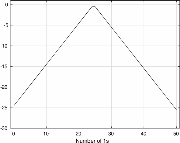

This function has two local minima but only one of them is global. As written above, the ACO algorithm considered is the MMAS, for which the pheromone bounds and ensure that at any time, there is a positive probability to visit each configuration, e.g. the global minimum. Therefore, with probability one this algorithm will find the solution. However, if it reaches a configuration with few s, it takes in average an enormous amount of time, not available in practice, to move towards the global minimum. Therefore, we expect that in this case the restart will be successful.
In Fig. 2, we show the estimated failure probability (f.p.) for the MMAS algorithm to minimize the pseudo-boolean function of Fig. 1 (tick line). In the same figure, the estimated f.p. of the RP is plotted versus the pseudo-time (thin line). We notice that there is a clear advantage to use the RP when compared to the standard MMAS.
We consider now an instance of the TSP with cities (att532). After five hundreds of thousands of iterations, the underlying algorithm has an estimated f.p. of ca. Instead, at the same value of the pseudo-time, the RP has a significantly lower f.p. ( ca), as clearly shown in Fig. 3. We remark that, until the value ca for the time or pseudo-time, the f.p. of the underlying algorithm is lower than the one of RP. This is due to the fact that the RP is still learning the optimal value of the restart time. After that, the trend is inverted: the RP overcomes the MMAS and gains two orders of magnitude for very large values of the pseudo-time.

We notice that the value approaches the optimal restart time . In fact, as an example, in Fig. 4, we show the denominator of the function at the end of a single RP execution. A global maximum appears at approximately the value of , the difference with the value of , computed from the estimate , being less than .

Finally in Fig. 5, we compare the f.p. curve for the RP with the one obtained applying the restart periodically with the estimated optimal restart time. We notice that this estimation requires much longer computation than to execute the RP. We remark that the RP curve starts to decrease significantly after the other one. This is due to the fact that the RP is still searching for the optimal value of the restart, whereas it is set from the beginning in the other (ideal) case. At about pseudo-time , the two f.p.s become almost equal. After that, the f.p. of the MMAS goes to zero faster, even if the difference between the two f.p.s remains less than ca. Finally, at pseudo-time , the f.p. of the RP is .
We notice that curves similar to those as in Fig. 3, 4 and 5 were obtained for all the other TSP instances considered. The relative results are shown in Table I.

| Instance | ACO algorithm | ACO f.p. | RP f.p. | |
|---|---|---|---|---|
| boolean50 | MMAS | |||
| pcb442 | MMAS-3opt | |||
| att532 | MMAS-3opt | |||
| lin318 | MMAS-2.5opt | |||
| d1291 | MMAS-3opt | |||
| d198 | MMAS-2.5opt |
By looking at the results in Table I, it is evident the advantage of using the RP instead of the underlying algorithm. In fact, for all instances, the f.p. of the RP is several orders of magnitude lower than the one of the underlying algorithm.
V Conclusions
Given a combinatorial optimization problem, it is often needed to apply stochastic algorithms exploring the space using a general criterion independent of the problem. Unfortunately, usually there is a positive probability that the algorithm remains in a sub-optimal solution. This problem can be afforded by applying periodic algorithm re-initializations. This strategy is called restart. Although it is often applied in practice, there are few works studying it theoretically. In particular, there are no theoretical information about how to choose a convenient value for the restart time.
In this paper, we propose a new procedure to optimize the restart and we study it theoretically. The iterative procedure starts by executing a certain number of replications of the underlying algorithm for a predefined time. Then, at any following iteration of the RP, we compute the minimum value of the objective function. Hence, for each time , we estimate the failure probability that we have not yet reached the value . After that, we compute the position of the first minimum of , which is a function of the failure probability. If is close to the end of the current execution time frame of the underlying algorithm , this last is increased; otherwise the number of replications is increased, which improves the estimate of . This is controlled by the parameter . The position of the minimum of corresponds to an “optimal value” of the restart time, that minimizes the expected time to find a solution.
The theory predicts that the algorithm will find the optimal value of the restart. In fact, the theorems proved demonstrate that, if tends to zero, has only one minimum at position and it is a strictly decreasing function until , then, with probability one, , and its first minimum converge to , and , respectively.
In this paper, we have shown some results obtained by applying the RP to several TSP instances with hundreds or thousands of cities. The results obtained have shown that the f.p. of the RP is several orders of magnitude lower than the one of the underlying algorithm, for equal computational cost. Therefore, given a certain computation resource, by applying the RP, we are far more confident that the result obtained is a solution of the COP instance analyzed. The procedure proposed could be improved preserving its performance and decreasing the computational cost. A possible way to do it is to increase the parameter along iterations. In fact, once we have a reasonably good estimate of , we would like to reduce the possibility that, by chance, we increase too much the time interval length. This can be done by increasing the value of .
Acknowledgments
The authors are very thankful to Prof. Mauro Piccioni for his very useful comments and suggestions and to Prof. Thomas Stützle for the ACOTSP code.
References
- [1] D. L. Applegate, R. M. Bixby, V. Chvátal, and W. J. Cook, The Traveling Salesman Problem. Princeton University Press, 2006.
- [2] C. Blum and A. Roli, “Metaheuristics in combinatorial optimization: overview and conceptual comparison,” ACM Computing Surveys, vol. 35, no. 3, pp. 268–308, 2003.
- [3] S. Kirkpatrick, C. D. Gelatt, and M. P. Vecchi, “Optimization by simulated annealing,” Science, vol. 220, no. 4598, pp. 671–680, 1983.
- [4] F. Glover, “Tabu search-part 1,” ORSA Journal of Computing, vol. 1, no. 3, pp. 190–206, 1989.
- [5] D. Goldberg, B. Korb, and K. Deb, “Messy genetic algorithms: Motivation, analysis, and first results,” Complex Systems, vol. 3, pp. 493–530, 1989.
- [6] M. Dorigo and T. Stützle, Ant Colony Optimization. MIT Press, 2004.
- [7] S. Geman and D. Geman, “Stochastic relaxation, gibbs distributions, and the bayesian restoration of images,” IEEE Transactions on Pattern Analysis and Machine Intelligence, vol. 6, no. 6, pp. 721–741, 1984.
- [8] L. T. Schmitt, “Fundamental study theory of genetic algorithms,” Theoretical Computer Science, vol. 259, pp. 1–61, 2001.
- [9] W. Gutjhar, “A generalized convergence result for the graph-based ant system,” Probability in the Engineering and Informational Sciences, vol. 17, pp. 545–569, 2003.
- [10] F. Neumann and C. Witt, “Runtime analysis of a simple ant colony optimization algorithm,” Algorithmica, vol. 54, pp. 243–255, 2007.
- [11] W. Gutjhar and G. Sebastiani, “Runtime analysis of ant colony optimization with best-so-far reinforcement’,” Methodology and Computing in Applied Probability, vol. 10, pp. 409–433, 2008.
- [12] M. Garvels and D. Kroese, “A comparison of restart implementations,” in Simulation Conference Proceedings. IEEE Computer Society Press, 1998, pp. 601–608.
- [13] ——, “On the entrance distribution in restart simulation,” in Proceedings of the Rare Event Simulation (RESIM ’99) Workshop. University of Twente, 1999, pp. 65–88.
- [14] A. Misevicius, “Restart-based genetic algorithm for the quadratic assignment problem,” in Research and Development in Intelligent Systems XXV, M. Bramer, M. Petridis, and F. Coenen, Eds. Springer-Verlag, 2009, pp. 91–104.
- [15] T. Hansen, “On the analysis of dynamic restart strategies for evolutionary algorithms,” in Proceedings of the 7th International Conference on Parallel Problem Solving from Nature. London: Springer-Verlag, 2002, pp. 33–43.
- [16] A. Van Moorsel and K. Wolter, “Analysis and algorithms for restart,” in Proceedings of the 1st International Conference on the Quantitative Evaluation of Systems (QEST), 2004, pp. 195–204.
- [17] L. Carvelli and G. Sebastiani, “Some issues of aco algorithm convergence,” in Ant Colony Optimization - Methods and Applications, A. Ostfeld, Ed. InTech, 2011, pp. 39–52.
- [18] T. Stützle and H. Hoos, “Max-min ant system,” Future Generation Computer Systems, vol. 16, pp. 889–914, 2000.