跳到论文正文
W Papers独立论文阅读器 arXiv:1709.06422 论文正文 计算阅读时间 · 0%
引用这篇论文根据当前论文元数据生成,正式投稿前建议核对。


License: arXiv.org perpetual non-exclusive license
arXiv:1709.06422v2 [math.NA] 27 Sep 2017
\pagespan

118 \copyrightinfo2004

A higher-order ensemble/proper orthogonal
decomposition method for the
nonstationary Navier-Stokes equations

Max Gunzburger Address:  Department of Scientific Computing, Florida State University, Tallahassee, FL 32306-4120 Email: mgunzburger@fsu.edu , Nan Jiang and Michael Schneier Address:  Department of Scientific Computing, Florida State University, Tallahassee, FL 32306-4120. Current address: Department of Mathematics and Statistics, Missouri University of Science and Technology, Rolla, MO 65409-0020 Email: jiangn@mst.edu Address:  Department of Scientific Computing, Florida State University, Tallahassee, FL 32306-4120 Email: mschneier89@gmail.com
Date: January 1, 2004 and, in revised form, March 22, 2004.
Abstract.

Partial differential equations (PDE) often involve parameters, such as viscosity or density. An analysis of the PDE may involve considering a large range of parameter values, as occurs in uncertainty quantification, control and optimization, inference, and several statistical techniques. The solution for even a single case may be quite expensive; whereas parallel computing may be applied, this reduces the total elapsed time but not the total computational effort. In the case of flows governed by the Navier-Stokes equations, a method has been devised for computing an ensemble of solutions. Recently, a reduced-order model derived from a proper orthogonal decomposition (POD) approach was incorporated into a first-order accurate in time version of the ensemble algorithm. In this work, we expand on that work by incorporating the POD reduced order model into a second-order accurate ensemble algorithm. Stability and convergence results for this method are updated to account for the POD/ROM approach. Numerical experiments illustrate the accuracy and efficiency of the new approach.

Key words and phrases: 
Navier-Stokes equations, ensemble computation, proper orthogonal decomposition, finite element methods
2000 Mathematics Subject Classification
35Q30, 65N30, 65M99

1. Introduction

In science and engineering, mathematical models are utilized to understand and predict the behavior of complex systems. Two common input data/parameters for these types of models include forcing terms and initial conditions. Often, for any number of reasons, there is a degree of uncertainty involved with the specification of such inputs. In order to obtain an accurate model we must incorporate such uncertainties into the governing equations and quantify their effects on the outputs of the simulation.

In this uncertainty quantification setting, one needs to determine many realizations of the outputs of the simulation in order to determine accurate statistical information about those outputs. A similar need occurs in other settings such as inference, optimization, and control and the need to determine solution ensembles arising in many applications, e.g., weather forecasting and turbulence modeling. Thus, in this work, we are interested in computing ensembles of solutions for the Navier-Stokes equations (NSE) with uncertainty present in the initial conditions and body forces. Specifically, for j=1,…,Jj=1,\ldots,J, we have

{utj+uj⋅∇uj−ν​△​uj+∇pj=fj​(x,t)∀x∈Ω×(0,T]∇⋅uj=0∀x∈Ω×(0,T]uj=0∀x∈∂Ω×(0,T]uj​(x,0)=uj,0​(x)∀x∈Ω,\left\{\begin{aligned} u_{t}^{j}+u^{j}\cdot\nabla u^{j}-\nu\triangle u^{j}+\nabla p^{j}&=f^{j}(x,t)&\quad\forall x\in\Omega\times(0,T]\\ \nabla\cdot u^{j}&=0&\quad\forall x\in\Omega\times(0,T]\\ u^{j}&=0&\quad\forall x\in\partial\Omega\times(0,T]\\ u^{j}(x,0)&=u^{j,0}(x)&\quad\forall x\in\Omega,\end{aligned}\right. (1)

where Ω⊂ℝd\Omega\subset\mathbb{R}^{d}, d=2,3d=2,3, is an open regular domain. In most settings, in order to guarantee a desired accuracy level in the outputs, a fine spatial resolution is usually required, which renders each realization to be computationally intensive. Traditionally, the simulation for each ensemble member is treated as a separate problem; therefore the focus has been to cut down on the total number of realizations needed. However, in recent works [11, 12, 13, 20], new algorithms were designed that allow for the realizations to be computed simultaneously at each time step. In those papers, the focus has been on creating algorithms which allow for the same linear system to be used for all right-hand sides. Hence, the need to solve a different linear system for each right-hand side is reduced to solving the a single system with many different right-hand sides. This is a well studied problem for which efficient block iterative methods already exist. A few examples of these include block CG [2], block QMR [3], and block GMRES [4].

The next natural step to take to further improve upon the efficiency of these ensemble algorithms is the introduction of reduced-order modeling (ROM) techniques. Specifically, we are interested in the implementation of the proper orthogonal decomposition (POD) approach into the ensemble framework. POD works by generally extracting from highly accurate numerical simulations or experimental data the most energetic modes in a given system.

One can then project the original problem onto these POD modes to obtain the Galerkin proper orthogonal decomposition (POD-G-ROM) approximation to the original problem. It has been shown for laminar flows [1, 10] that it is possible to obtain a good approximation with few POD modes, hence the corresponding POD-G-ROM only requires the solution of a small linear system. Recently, in [6], a POD-G-ROM ensemble algorithm based on the first-order accurate in time ensemble algorithm first introduced in [13] was developed. However, in applications that require long-term time integration, such as climate and ocean forecasting, higher-order methods are highly desirable. For this reason, in this paper we expand on the work of [6] by introducing the POD method into the second-order ensemble algorithm introduced in [11].

2. Notation and preliminaries

We denote by ∥⋅∥\|\cdot\| and (⋅,⋅)(\cdot,\cdot) the L2​(Ω)L^{2}(\Omega) norm and inner product, respectively, and by ∥⋅∥Lp\|\cdot\|_{L^{p}} and ∥⋅∥Wpk\|\cdot\|_{W_{p}^{k}} the Lp​(Ω)L^{p}(\Omega) and Sobolev Wpk​(Ω)W^{k}_{p}(\Omega) norms, respectively. Hk​(Ω)=W2k​(Ω)H^{k}(\Omega)=W_{2}^{k}(\Omega) with norm ∥⋅∥k\|\cdot\|_{k}. For a function v⁡(x,t)v(x,t) that is well defined on Ω×[0,T]\Omega\times[0,T], we define the norms

|||v|||2,s:=(∫0T∥v(⋅,t)∥s2dt)12and∥|v|||∞,s:=ess sup[0,T]∥v(⋅,t)∥s.|||v|||_{2,s}:=\Big(\int_{0}^{T}\|v(\cdot,t)\|_{s}^{2}dt\Big)^{\frac{1}{2}}\qquad\text{and}\qquad\||v|||_{\infty,s}:=\text{ess\,sup}_{[0,T]}\|v(\cdot,t)\|_{s}.

The space H−1​(Ω)H^{-1}(\Omega) denotes the dual space of bounded linear functionals defined on H01​(Ω)={v∈H1​(Ω):v=0​ on ​∂Ω}H^{1}_{0}(\Omega)=\{v\in H^{1}(\Omega)\,:\,v=0\mbox{ on }\partial\Omega\}; this space is equipped with the norm

‖f‖−1=sup0≠v∈X(f,v)‖∇v‖∀f∈H−1​(Ω).\|f\|_{-1}=\sup_{0\neq v\in X}\frac{(f,v)}{\|\nabla v\|}\quad\forall f\in H^{-1}(\Omega).

The solutions spaces XX for the velocity and QQ for the pressure are respectively defined as

X:=\displaystyle X:= [H01​(Ω)]d={v∈[L2​(Ω)]d:∇v∈[L2​(Ω)]d×d​and​v=0​on​∂Ω}\displaystyle[H^{1}_{0}(\Omega)]^{d}=\{v\in[L^{2}(\Omega)]^{d}\,:\,\nabla v\in[L^{2}(\Omega)]^{d\times d}\ \text{and}\ v=0\ \text{on}\ \partial\Omega\}
Q:=\displaystyle Q:= L02​(Ω)={q∈L2​(Ω):∫Ωq​dx=0}.\displaystyle L^{2}_{0}(\Omega)=\Big\{q\in L^{2}(\Omega)\,:\,\int_{\Omega}qdx=0\Big\}.

A weak formulation of (1) is given as follows: for j=1,…,Jj=1,\ldots,J, find uj:(0,T]→Xu^{j}:(0,T]\rightarrow X and pj:(0,T]→Qp^{j}:(0,T]\rightarrow Q such that, for almost all t∈(0,T]t\in(0,T], satisfy

{(utj,v)+(uj⋅∇uj,v)+ν⁡(∇uj,∇v)−(pj,∇⋅v)=(fj,v)∀v∈X(∇⋅uj,q)=0∀q∈Quj​(x,0)=uj,0​(x).\left\{\begin{aligned} (u_{t}^{j},v)+(u^{j}\cdot\nabla u^{j},v)+\nu(\nabla u^{j},\nabla v)-(p^{j},\nabla\cdot v)&=(f^{j},v)&\quad\forall v\in X\\ (\nabla\cdot u^{j},q)&=0&\quad\forall q\in Q\\ u^{j}(x,0)&=u^{j,0}(x).&\end{aligned}\right. (2)

The subspace of XX consisting of weakly divergence-free functions is defined as

V:={v∈X:(∇⋅v,q)=0​∀q∈Q}⊂X.V:=\{v\in X\,:\,(\nabla\cdot v,q)=0\,\,\forall q\in Q\}\subset X.

We denote conforming velocity and pressure finite element spaces based on a regular triangulation of Ω\Omega having maximum triangle diameter hh by Xh⊂XX_{h}\subset X and Qh⊂Q.Q_{h}\subset Q. We assume that the pair of spaces (Xh,Qh)(X_{h},Q_{h}) satisfy the discrete inf-sup (or L​B​BhLBB_{h}) condition required for stability of finite element approximations; we also assume that the finite element spaces satisfy the approximation properties

infvh∈Xh‖v−vh‖\displaystyle\inf_{v_{h}\in X_{h}}\|v-v_{h}\| ≤C​hs+1\displaystyle\leq Ch^{s+1} ∀v∈[Hs+1​(Ω)]d\displaystyle\forall v\in[H^{s+1}(\Omega)]^{d}
infvh∈Xh‖∇(v−vh)‖\displaystyle\inf_{v_{h}\in X_{h}}\|\nabla(v-v_{h})\| ≤C​hs\displaystyle\leq Ch^{s} ∀v∈[Hs+1​(Ω)]d\displaystyle\forall v\in[H^{s+1}(\Omega)]^{d}
infqh∈Qh‖q−qh‖\displaystyle\inf_{q_{h}\in Q_{h}}\|q-q_{h}\| ≤C​hs\displaystyle\leq Ch^{s} ∀q∈Hs​(Ω),\displaystyle\forall q\in H^{s}(\Omega),

where CC is a positive constant that is independent of hh. The Taylor-Hood element pairs (PsP^{s}-Ps−1P^{s-1}), s≥2s\geq 2, are one common choice for which the L​B​BhLBB_{h} stability condition and the approximation estimates hold [5, 7].

In this paper, we solve the NSE (1) (to generate snapshots) using a second-order time stepping scheme (e.g., Crank-Nicolson). Thus, we assume the finite element approximations satisfy the error estimates, which are used in the analysis in Section 5,

‖u−uh‖≤C⁡(hs+1+Δ​t2)\displaystyle\|u-u_{h}\|\leq C(h^{s+1}+\Delta t^{2})
‖∇(u−uh)‖≤C⁡(hs+Δ​t2).\displaystyle\|\nabla(u-u_{h})\|\leq C(h^{s}+\Delta t^{2}).

We define the trilinear form

b⁡(w,u,v)=(w⋅∇u,v)∀u,v,w∈[H1​(Ω)]db(w,u,v)=(w\cdot\nabla u,v)\qquad\forall u,v,w\in[H^{1}(\Omega)]^{d}

and the explicitly skew-symmetric trilinear form given by

b∗​(w,u,v):=12​(w⋅∇u,v)−12​(w⋅∇v,u)∀u,v,w∈[H1​(Ω)]db^{\ast}(w,u,v):=\frac{1}{2}(w\cdot\nabla u,v)-\frac{1}{2}(w\cdot\nabla v,u)\qquad\forall u,v,w\in[H^{1}(\Omega)]^{d}

which satisfies the bounds [18]

b∗​(w,u,v)≤C​‖∇w‖|∇u|(‖v‖​‖∇v‖)1/2∀u,v,w∈X\displaystyle b^{\ast}(w,u,v)\leq C\|\nabla w\|\|\nabla u\|(\|v\|\|\nabla v\|)^{1/2}\qquad\forall u,v,w\in X (3)
b∗​(w,u,v)≤C​(‖w‖​‖∇w‖)1/2​‖∇u‖​‖∇v‖∀u,v,w∈X.\displaystyle b^{\ast}(w,u,v)\leq C(\|w\|\|\nabla w\|)^{1/2}\|\nabla u\|\|\nabla v\|\qquad\forall u,v,w\in X. (4)

We also have for ∀uh,vh,wh∈Xh\forall u_{h},v_{h},w_{h}\in X_{h}

b∗​(wh,uh,vh)=∫Ωwh⋅∇uh⋅vh​𝑑x+12​∫Ω(∇⋅wh)​(uh⋅vh)​𝑑x.\displaystyle b^{\ast}(w_{h},u_{h},v_{h})=\int_{\Omega}w_{h}\cdot\nabla u_{h}\cdot v_{h}dx+\frac{1}{2}\int_{\Omega}(\nabla\cdot w_{h})(u_{h}\cdot v_{h})dx. (5)

We also define the discretely divergence-free space VhV_{h} as

Vh:={vh∈Xh:(∇⋅vh,qh)=0​∀qh∈Qh}⊂X.V_{h}:=\{v_{h}\in X_{h}\,:\,(\nabla\cdot v_{h},q_{h})=0\,\,\forall q_{h}\in Q_{h}\}\subset X.

In most cases, and for the Taylor-Hood element pair in particular, Vh⊄VV_{h}\not\subset V, i.e., discretely divergence-free functions are not divergence-free.

In this work, we focus on extending our previously developed second-order accurate approximation for computing the solution of an ensemble of Navier-Stokes equations. These methods require a new definition for the ensemble mean as opposed to that used in [6].

Definition 2.1.

Let tn=n​Δ​tt^{n}=n\Delta t, n=0,1,2,…,Nn=0,1,2,\ldots,N, where N:=T/Δ​tN:=T/\Delta t, denote a partition of the interval [0,T][0,T]. Let |⋅||\cdot| denote the Euclidian length of a vector. For j=1,…,Jj=1,\ldots,J and n=0,1,2,…,Nn=0,1,2,\ldots,N, let uj,n​(x):=uj​(x,tn)u^{j,n}(x):=u^{j}(x,t^{n}). Then, the ensemble mean, fluctuation about the mean, and magnitude of fluctuation are respectively defined, for n=1,2,…,Nn=1,2,\ldots,N, by

{<u>n:=1J​∑j=1J(2​uj,n−uj,n−1)u′j,n:=2uj,n−uj,n−1−<u>n|u′n|:=(∑j=1J|u′j,n|2)12.\left\{\begin{aligned} <u>^{n}:&=\frac{1}{J}\sum_{j=1}^{J}\left(2u^{j,n}-u^{j,n-1}\right)\\ u^{\prime j,n}:&=2u^{j,n}-u^{j,n-1}-<u>^{n}\\ |u^{\prime n}|:&=\Big(\sum_{j=1}^{J}|u^{\prime j,n}|^{2}\Big)^{\frac{1}{2}}.\end{aligned}\right.

The full space-time discrete model given in [14] that we refer to as EnB-full is given as: for j=1,…,Jj=1,\ldots,J, given uhj,0∈Xhu^{j,0}_{h}\in X_{h} and uhj,1∈Xhu^{j,1}_{h}\in X_{h}, for n=1,2,…,N−1n=1,2,\ldots,N-1 find uhj,n+1∈Xhu^{j,n+1}_{h}\in X_{h} and phj,n+1∈Qhp_{h}^{j,n+1}\in Q_{h} satisfying

​(3​uhj,n+1−4​uhj,m+uhj,n−12​Δ​t,vh)+b∗(<uh>n,uj,n+1h,vh)+ν(∇uj,n+1h,∇vh)+b∗​(uh′j,n,2​uhj,n−uhj,n−1,vh)−(phj,n+1,∇⋅vh)=(fj,n+1,vh)∀vh∈Xh(∇⋅uhj,n+1,qh)=0∀qh∈Qh.\emph{}\begin{aligned} &\Big(\frac{3u^{j,n+1}_{h}-4u^{j,m}_{h}+u^{j,n-1}_{h}}{2\Delta t},v_{h}\Big)+b^{\ast}(<u_{h}>^{n},u^{j,n+1}_{h},v_{h})+\nu(\nabla u^{j,n+1}_{h},\nabla v_{h})\\ &+b^{\ast}(u^{\prime j,n}_{h},2u^{j,n}_{h}-u^{j,n-1}_{h},v_{h})-(p^{j,n+1}_{h},\nabla\cdot v_{h})=(f^{j,n+1},v_{h})\quad\forall v_{h}\in X_{h}\\ &\qquad\quad(\nabla\cdot u_{h}^{j,n+1},q_{h})=0\qquad\forall q_{h}\in Q_{h}.\end{aligned} (6)

3. Proper orthogonal decomposition (POD) method

We next briefly discuss the POD method and how we can apply it to the previously discussed ensemble algorithm. For a more in depth description, see [8, 1, 16, 15]. In Section 6, the results of numerical experiments are given to illustrate the efficacy of our new algorithm.

Given a positive integer NSN_{S}, let 0=t0<t1<⋯<tNS=T0=t_{0}<t_{1}<\cdots<t_{N_{S}}=T denote a uniform partition of the time interval [0,T][0,T]. For j=1,…,JSj=1,\ldots,J_{S}, we select JSJ_{S} different initial conditions uj,0​(x)u^{j,0}(x) and denote by uh,Sj,m​(x)∈Xhu_{h,S}^{j,m}(x)\in X_{h}, j=1,…,JSj=1,\ldots,J_{S}, m=1,…,NSm=1,\ldots,N_{S}, the finite element approximation to (2) evaluated at t=tmt=t_{m}, m=1,…,NSm=1,\ldots,N_{S}, corresponding to an approximate initial condition uhj,0​(x)∈Xhu_{h}^{j,0}(x)\in X_{h} such as the XhX_{h}-interpolant of uj,0​(x)u^{j,0}(x). We then define the space spanned by the JS​(NS+1)J_{S}(N_{S}+1) discrete snapshots as

Xh,S:=span​{uh,Sj,m​(x)}j=1,m=0JS,NS⊂Vh⊂Xh.X_{h,S}:=\text{span}\{u_{h,S}^{j,m}(x)\}_{j=1,m=0}^{J_{S},N_{S}}\subset V_{h}\subset X_{h}.

Denoting by u→Sj,m\vec{u}_{S}^{j,m} the vector of coefficients corresponding to the finite element function uh,Sj,m​(x)u_{h,S}^{j,m}(x), where K=dimXhK=\dim X_{h}, we define the K×JS​(NS+1)K\times J_{S}(N_{S}+1) snapshot matrix 𝔸\mathbb{A} as

𝔸=(u→S1,0,u→S1,1,…,u→S1,NS,u→S2,0,u→S2,1,…,u→S2,NS,…,u→SJS,0,u→SJS,1,…,u→SJS,NS),\mathbb{A}=\big(\vec{u}_{S}^{1,0},\vec{u}_{S}^{1,1},\ldots,\vec{u}_{S}^{1,N_{S}},\vec{u}_{S}^{2,0},\vec{u}_{S}^{2,1},\ldots,\vec{u}_{S}^{2,N_{S}},\ldots,\vec{u}_{S}^{J_{S},0},\vec{u}_{S}^{J_{S},1},\ldots,\vec{u}_{S}^{J_{S},N_{S}}\big),

i.e., the columns of 𝔸\mathbb{A} are the finite element coefficient vectors corresponding to the discrete snapshots. The POD method then seeks a low dimensional basis

XR:=span​{φi}i=1R⊂Xh,S⊂Vh⊂XhX_{R}:=\text{span}\{{\varphi}_{i}\}_{i=1}^{R}\subset X_{h,S}\subset V_{h}\subset X_{h}

which can approximate the snapshot data. This basis can be determined by finding an orthonormal basis {φi}i=1S\{\varphi_{i}\}_{i=1}^{S} for Xh,SX_{h,S} such that for all R∈{1,…,S}R\in\{1,\ldots,S\}, {φi}i=1R\{\varphi_{i}\}_{i=1}^{R}, solves the constrained minimization problem

min∑k=1JS∑l=0NS∥uh,sk,l−∑j=1R(uh,sk,l,φj)φj∥2\displaystyle\min\sum_{k=1}^{J_{S}}\sum_{l=0}^{N_{S}}\Big\|u_{h,s}^{k,l}-\sum_{j=1}^{R}(u_{h,s}^{k,l},\varphi_{j})\varphi_{j}\Big\|^{2} (7)
subject to ​(φi,φj)=δi​jfor i,j=1,…,R,\displaystyle\text{subject to }(\varphi_{i},\varphi_{j})=\delta_{ij}\quad\mbox{for $i,j=1,\ldots,R$},

where δi​j\delta_{ij} denotes the Kronecker delta and the minimization is with respect to all orthonormal bases for Xh,SX_{h,S}. We define the JS​(NS+1)×JS​(NS+1)J_{S}(N_{S}+1)\times J_{S}(N_{S}+1) correlation matrix ℂ=𝔸T​𝕄​𝔸\mathbb{C}=\mathbb{A}^{T}\mathbb{M}\mathbb{A}, where 𝕄\mathbb{M} denotes the Gram matrix corresponding to full finite element space. Then, the problem (7) is equivalent to determine the RR dominant eigenpairs {λi,a→i}\{\lambda_{i},\vec{a}_{i}\} satifying

ℂa→i=λia→i,|a→i|=1,a→Tia→j=0ifi≠j,andλi≥λi−1>0,\mathbb{C}\vec{a}_{i}=\lambda_{i}\vec{a}_{i},\quad|\vec{a}_{i}|=1,\quad\vec{a}^{T}_{i}\vec{a}_{j}=0\ \text{if}\ i\neq j,\quad\text{and}\quad\lambda_{i}\geq\lambda_{i-1}>0,

where |⋅||\cdot| denotes the Euclidean norm of a vector. The finite element coefficient vectors corresponding to the POD basis functions are then given by

φ→i=1λi𝔸a→i,i=1,…,R.\vec{\varphi}_{i}=\frac{1}{\sqrt{\lambda_{i}}}\mathbb{A}\vec{a}_{i},\ \ \ i=1,\ldots,R.

3.1. POD-ensemble based reduced-order model

We next show how the POD method can be used to construct a reduced-order model within the framework of the EnB-full algorithm. The formulation of the POD approximation is identical to that of the full finite element approximation. Instead of seeking a solution in the finite element space XhX_{h}, we seek a solution in the POD space XRX_{R} using the basis {φi}i=1R.\{\varphi_{i}\}_{i=1}^{R}. Now, for j=1,…,Jj=1,\ldots,J, we define the POD approximation of the initial conditions as uRj,0​(x)=∑i=1R(uj,0,φi)​φi​(x)∈XRu_{R}^{j,0}(x)=\sum_{i=1}^{R}(u^{j,0},{\varphi}_{i})\varphi_{i}(x)\in X_{R} and POD approximation of the of uj,1u^{j,1} as uRj,1​(x)=∑i=1R(uhj,1,φi)​φi​(x)∈XRu_{R}^{j,1}(x)=\sum_{i=1}^{R}(u^{j,1}_{h},{\varphi}_{i})\varphi_{i}(x)\in X_{R}, where uhj,1u_{h}^{j,1} denotes a finite element approximation of uj,1u^{j,1} using a second-order (or higher-order) time stepping method such that ‖uj,1−uhj,1‖1=O⁡(hs+Δ​t2)\|u^{j,1}-u_{h}^{j,1}\|_{1}=O(h^{s}+\Delta t^{2}) accurate or better. We then pose the following problem: given uRj,0​(x),uRj,1∈XRu_{R}^{j,0}(x),u_{R}^{j,1}\in X_{R}, for n=0,1,…,N−1n=0,1,\ldots,N-1 and for j=1,…,Jj=1,\ldots,J, find uRj,n+1∈XRu_{R}^{j,n+1}\in X_{R} satisfying

(3​uRj,n+1−4​uRj,n+uRj,n−12​Δ​t,φ)+b∗(<uR>n,uRj,n+1,φ)\displaystyle\big(\frac{3u_{R}^{j,n+1}-4u_{R}^{j,n}+u_{R}^{j,n-1}}{2\Delta t},\varphi\big)+b^{\ast}(<u_{R}>^{n},u_{R}^{j,n+1},\varphi) (8)
+b∗​(uR′j,n,2​uRj,n−uRj,n−1,φ)+ν⁡(∇uRj,n+1,∇φ)=(fj,n+1,φ)∀φ∈XR.\displaystyle+b^{\ast}(u_{R}^{\prime j,n},2u_{R}^{j,n}-u_{R}^{j,n-1},\varphi)+\nu(\nabla u_{R}^{j,n+1},\nabla\varphi)=(f^{j,n+1},\varphi)\qquad\forall\varphi\in X_{R}.

We refer to (8) as EnB-POD. We note that because XR⊂VhX_{R}\subset V_{h}, the POD basis is discretely divergence free by construction. Therefore, there is no pressure term present in (8) and the only unknown in our system is the approximate velocity vector.

4. Stability of EnB-POD

In this section, we present results pertaining to the conditional, nonlinear, longterm stability of solutions of (8).

We denote by ∥|⋅∥|2\|\hskip-1.0pt|\cdot\|\hskip-1.0pt|_{2} the spectral norm for symmetric matrices and let 𝕄R{\mathbb{M}}_{R} denote the R×RR\times R POD mass matrix with entries [𝕄R]i,i′=(φi,φi′)[{\mathbb{M}}_{R}]_{i,i^{\prime}}=(\varphi_{i},\varphi_{i^{\prime}}) and 𝕊R{\mathbb{S}}_{R} denote the R×RR\times R matrix with entries [𝕊R]i,i′=[𝕄R]i,i′+ν⁡(∇φi,∇φi′)[{\mathbb{S}}_{R}]_{i,i^{\prime}}=[{\mathbb{M}}_{R}]_{i,i^{\prime}}+\nu(\nabla\varphi_{i},\nabla\varphi_{i^{\prime}}), i,i′=1,…,Ri,i^{\prime}=1,\ldots,R. By construction the POD basis functions are orthonormal with respect to the L2​(Ω)L^{2}(\Omega) inner product, hence the mass matrix is actually the identity matrix and ∥|𝕄R∥|2=∥|𝕄R−1∥|2=1\|\hskip-1.0pt|{\mathbb{M}}_{R}\|\hskip-1.0pt|_{2}=\|\hskip-1.0pt|{\mathbb{M}}_{R}^{-1}\|\hskip-1.0pt|_{2}=1. Then, we have the inequality [16]

∥∇φ∥≤(∥|𝕊R∥|2∥|𝕄R−1∥|2)1/2∥φ∥≤∥|𝕊R∥|21/2∥φ∥∀φ∈XR.\|\nabla\varphi\|\leq\big(\|\hskip-1.0pt|{\mathbb{S}}_{R}\|\hskip-1.0pt|_{2}\|\hskip-1.0pt|{\mathbb{M}}_{R}^{-1}\|\hskip-1.0pt|_{2}\big)^{1/2}\|\varphi\|\leq\|\hskip-1.0pt|{\mathbb{S}}_{R}\|\hskip-1.0pt|_{2}^{1/2}\|\varphi\|\qquad\forall\varphi\in X_{R}. (9)

We now show that EnB-POD is stable under a time-step condition similar to that for EnB-full except the norm of the POD stiffness matrix now plays a role in the stability condition.

Theorem 4.1

For the method (8), suppose that

C∥|𝕊R∥|212Δ​tν∥∇u′j,nR∥2≤1for j=1,…,J.C\|\hskip-1.0pt|{\mathbb{S}}_{R}\|\hskip-1.0pt|_{2}^{\frac{1}{2}}\frac{\Delta t}{\nu}\|\nabla u^{\prime j,n}_{R}\|^{2}\leq 1\qquad\mbox{for $j=1,\ldots,J$}. (10)

Then, for n=0,…,N−1n=0,\ldots,N-1

14​‖uRj,n‖2+14​‖2​uRj,n−uRj,n−1‖2+Δ​t​ν4​∑n′=1n−1‖∇uRj,n′+1‖2\displaystyle\frac{1}{4}\|u^{j,n}_{R}\|^{2}+\frac{1}{4}\|2u^{j,n}_{R}-u^{j,n-1}_{R}\|^{2}+\frac{\Delta t\nu}{4}\sum_{n^{\prime}=1}^{n-1}\|\nabla u_{R}^{j,n^{\prime}+1}\|^{2} (11)
≤Δ​tν​∑n′=1n−1‖fj,n′+1‖−12+14​‖uRj,1‖2+14​‖2​uRj,1−uRj,0‖2.\displaystyle\leq\frac{\Delta t}{\nu}\sum_{n^{\prime}=1}^{n-1}\|f^{j,n^{\prime}+1}\|^{2}_{-1}+\frac{1}{4}\|u^{j,1}_{R}\|^{2}+\frac{1}{4}\|2u^{j,1}_{R}-u^{j,0}_{R}\|^{2}.
Proof.

The proof is very similar to that for [11, Theorem 1], the main difference being the use of a different basis function. Setting φ=uRj,n+1\varphi=u^{j,n+1}_{R}, using skew-symmetry of the trilinear form, and applying Young’s inequality to the right-hand side, we have.

14​(‖uRj,n+1‖2+‖2​uRj,n+1−uRj,n‖2)−14​(‖uRj,n‖2+‖2​uRj,n−uRj,n−1‖2)\displaystyle\frac{1}{4}\left(\|u^{j,n+1}_{R}\|^{2}+\|2u^{j,n+1}_{R}-u^{j,n}_{R}\|^{2}\right)-\frac{1}{4}\left(\|u^{j,n}_{R}\|^{2}+\|2u^{j,n}_{R}-u^{j,n-1}_{R}\|^{2}\right) (12)
+14​‖uRj,n+1−2​uRj,n+uRj,n−1‖2+Δ​t​b∗​(uR′j,n,2​uRj,n−uRj,n−1,uRj,n+1)\displaystyle+\frac{1}{4}\|u^{j,n+1}_{R}-2u^{j,n}_{R}+u^{j,n-1}_{R}\|^{2}+\Delta tb^{\ast}(u^{\prime j,n}_{R},2u^{j,n}_{R}-u^{j,n-1}_{R},u^{j,n+1}_{R})
+ν​Δ​t​‖∇uRj,n+1‖2≤ν​Δ​t4​‖∇uRj,n+1‖2+Δ​tν​‖fj,n+1‖−12.\displaystyle+\nu\Delta t\|\nabla u_{R}^{j,n+1}\|^{2}\leq\frac{\nu\Delta t}{4}\|\nabla u^{j,n+1}_{R}\|^{2}+\frac{\Delta t}{\nu}\|f^{j,n+1}\|^{2}_{-1}.

We can then rewrite, using skew symmetry, the trilinear term as

b∗​(uR′j,n,2​uRj,n−uRj,n−1,uRj,n+1)=b∗​(uR′j,n,uRj,n+1,uRj,n+1−2​uRj,n+uRj,n−1).\displaystyle b^{\ast}(u_{R}^{\prime j,n},2u_{R}^{j,n}-u_{R}^{j,n-1},u_{R}^{j,n+1})=b^{\ast}(u^{\prime j,n}_{R},u^{j,n+1}_{R},u^{j,n+1}_{R}-2u^{j,n}_{R}+u^{j,n-1}_{R}).

Now bounding the trilinear form using (9)

Δ​t​b∗​(uR′j,n,uRj,n+1,uRj,n+1−2​uRj,n+uRj,n−1)\displaystyle\Delta tb^{\ast}(u^{\prime j,n}_{R},u^{j,n+1}_{R},u^{j,n+1}_{R}-2u^{j,n}_{R}+u^{j,n-1}_{R}) (13)
≤CΔt∥∇u′j,nR∥||∇uj,n+1R∥∥uj,n+1R−2uj,nR+uj,n−1R∥12∥∇(uj,n+1R−2uj,nR+uj,n−1R)∥12\displaystyle\leq C\Delta t\|\nabla u^{\prime j,n}_{R}\|||\nabla u^{j,n+1}_{R}\|\|u^{j,n+1}_{R}-2u^{j,n}_{R}+u^{j,n-1}_{R}\|^{\frac{1}{2}}\|\nabla(u^{j,n+1}_{R}-2u^{j,n}_{R}+u^{j,n-1}_{R})\|^{\frac{1}{2}}
≤CΔt∥∇u′j,nR∥||∇uj,n+1R∥∥uj,n+1R−2uj,nR+uj,n−1R∥∥|𝕊R∥|214.\displaystyle\leq C\Delta t\|\nabla u^{\prime j,n}_{R}\|||\nabla u^{j,n+1}_{R}\|\|u^{j,n+1}_{R}-2u^{j,n}_{R}+u^{j,n-1}_{R}\|\|\hskip-1.0pt|{\mathbb{S}}_{R}\|\hskip-1.0pt|_{2}^{\frac{1}{4}}.

Applying Young’s inequality gives

C\displaystyle C Δt∥∇u′j,nR∥||∇uj,n+1R∥∥uj,n+1R−2uj,nR+uj,n−1R∥|||𝕊R∥|214\displaystyle\Delta t\|\nabla u^{\prime j,n}_{R}\|||\nabla u^{j,n+1}_{R}\|\|u^{j,n+1}_{R}-2u^{j,n}_{R}+u^{j,n-1}_{R}\|||\hskip-1.0pt|{\mathbb{S}}_{R}\|\hskip-1.0pt|_{2}^{\frac{1}{4}}
≤CΔt2∥∇u′j,nR∥2∥∇uj,n+1R∥2∥|𝕊R∥|212+14∥uj,n+1R−2uj,nR+uj,n−1R∥2.\displaystyle\leq C\Delta t^{2}\|\nabla u^{\prime j,n}_{R}\|^{2}\|\nabla u^{j,n+1}_{R}\|^{2}\|\hskip-1.0pt|{\mathbb{S}}_{R}\|\hskip-1.0pt|_{2}^{\frac{1}{2}}+\frac{1}{4}\|u^{j,n+1}_{R}-2u^{j,n}_{R}+u^{j,n-1}_{R}\|^{2}.

Using this bound we then combine like terms. (12) becomes

14​(‖uRj,n+1‖2+‖2​uRj,n+1−uRj,n‖2)−14​(‖uRj,n‖2+‖2​uRj,n−uRj,n−1‖2)\displaystyle\frac{1}{4}\left(\|u^{j,n+1}_{R}\|^{2}+\|2u^{j,n+1}_{R}-u^{j,n}_{R}\|^{2}\right)-\frac{1}{4}\left(\|u^{j,n}_{R}\|^{2}+\|2u^{j,n}_{R}-u^{j,n-1}_{R}\|^{2}\right) (14)
+ν​Δ​t4∥∇uRj,n+1∥2+ν​Δ​t2(1−C∥|𝕊R∥|212Δ​tν∥∇u′j,nR∥2)∥∇uj,n+1R∥\displaystyle+\frac{\nu\Delta t}{4}\|\nabla u_{R}^{j,n+1}\|^{2}+\frac{\nu\Delta t}{2}\left(1-C\|\hskip-1.0pt|{\mathbb{S}}_{R}\|\hskip-1.0pt|_{2}^{\frac{1}{2}}\frac{\Delta t}{\nu}\|\nabla u^{\prime j,n}_{R}\|^{2}\right)\|\nabla u^{j,n+1}_{R}\|
≤Δ​tν​‖fj,n+1‖−12.\displaystyle\leq\frac{\Delta t}{\nu}\|f^{j,n+1}\|^{2}_{-1}.

Now under condition (10), it follows that

ν​Δ​t2(1−C∥|𝕊R∥|212Δ​tν∥∇uR′j,n∥2)∥∇uRj,n+1∥≥0\frac{\nu\Delta t}{2}\left(1-C\|\hskip-1.0pt|{\mathbb{S}}_{R}\|\hskip-1.0pt|_{2}^{\frac{1}{2}}\frac{\Delta t}{\nu}\|\nabla u^{\prime j,n}_{R}\|^{2}\right)\|\nabla u^{j,n+1}_{R}\|\geq 0

(14) and then simplifies to

14​(‖uRj,n+1‖2+‖2​uRj,n+1−uRj,n‖2)−14​(‖uRj,n‖2+‖2​uRj,n−uRj,n−1‖2)\displaystyle\frac{1}{4}\left(\|u^{j,n+1}_{R}\|^{2}+\|2u^{j,n+1}_{R}-u^{j,n}_{R}\|^{2}\right)-\frac{1}{4}\left(\|u^{j,n}_{R}\|^{2}+\|2u^{j,n}_{R}-u^{j,n-1}_{R}\|^{2}\right)
+ν​Δ​t4​‖∇uRj,n+1‖2≤Δ​tν​‖fj,n+1‖−12.\displaystyle+\frac{\nu\Delta t}{4}\|\nabla u_{R}^{j,n+1}\|^{2}\leq\frac{\Delta t}{\nu}\|f^{j,n+1}\|^{2}_{-1}.

Summing up the above inequality results in (11). ∎

4.1. Improving the time-step condition

While Theorem 4.1 is true universally in two and three dimensions, there are also certain cases for which we can improve upon our estimate. We are specifically interested in the three-dimensional case for which we make use of the Sobolev embedding inequality: for v∈Xv\in X and d=3d=3, the L6L^{6} norm satisfies [17]

‖v‖L6≤Cs​e​‖∇v‖∀v∈X,\|v\|_{L^{6}}\leq C_{se}\|\nabla v\|\quad\forall v\in X, (15)

where the constant Cs​e=23C_{se}=\frac{2}{\sqrt{3}}. In the following stability estimate, we see that instead of needing to control the gradient of fluctuations about the mean, we now are only concerned with L3L^{3} fluctuations about the mean.

Theorem 4.2

Consider the method (8) when d=3d=3. Suppose that

Cs​e2​‖𝕊R‖​Δ​tν​‖uR′j,n‖L32≤1for j=1,…,J.C_{se}^{2}\|\mathbb{S}_{R}\|\frac{\Delta t}{\nu}\|u^{\prime j,n}_{R}\|_{L^{3}}^{2}\leq 1\qquad\mbox{for $j=1,\ldots,J$}. (16)

Then, for n=0,…,N−1n=0,\ldots,N-1

14​‖uRj,n‖2+14​‖2​uRj,n−uRj,n−1‖2+Δ​t​ν4​∑n′=1n−1‖∇uRj,n′+1‖2\displaystyle\frac{1}{4}\|u^{j,n}_{R}\|^{2}+\frac{1}{4}\|2u^{j,n}_{R}-u^{j,n-1}_{R}\|^{2}+\frac{\Delta t\nu}{4}\sum_{n^{\prime}=1}^{n-1}\|\nabla u_{R}^{j,n^{\prime}+1}\|^{2} (17)
≤Δ​tν​∑n′=1n−1‖fj,n′+1‖−12+14​‖uRj,1‖2+14​‖2​uRj,1−uRj,0‖2.\displaystyle\leq\frac{\Delta t}{\nu}\sum_{n^{\prime}=1}^{n-1}\|f^{j,n^{\prime}+1}\|^{2}_{-1}+\frac{1}{4}\|u^{j,1}_{R}\|^{2}+\frac{1}{4}\|2u^{j,1}_{R}-u^{j,0}_{R}\|^{2}.
Proof.

By (5) and Ho¨\ddot{o}lders’ inequality, we have

b∗(u′j,nR,\displaystyle b^{\ast}(u^{\prime j,n}_{R}, OPENuRj,n+1,uRj,n+1−2​uRj,n+uRj,n−1)\displaystyle u^{j,n+1}_{R},u^{j,n+1}_{R}-2u^{j,n}_{R}+u^{j,n-1}_{R})
≤12​‖uR′j,n‖L3​‖∇uRj,n+1‖L2​‖uRj,n+1−2​uRj,n+uRj,n−1‖L6\displaystyle\leq\frac{1}{2}\|u^{\prime j,n}_{R}\|_{L^{3}}\|\nabla u^{j,n+1}_{R}\|_{L^{2}}\|u^{j,n+1}_{R}-2u^{j,n}_{R}+u^{j,n-1}_{R}\|_{L^{6}}
+12​‖uR′j,n‖L3​‖uRj,n+1‖L6​‖∇(uRj,n+1−2​uRj,n+uRj,n−1)‖L2.\displaystyle+\frac{1}{2}\|u^{\prime j,n}_{R}\|_{L^{3}}\|u^{j,n+1}_{R}\|_{L^{6}}\|\nabla(u^{j,n+1}_{R}-2u^{j,n}_{R}+u^{j,n-1}_{R})\|_{L^{2}}.

Now applying (15) and (9) we have

∥uj,n+1R−2uj,nR+uj,n−1R∥L6≤Cs​e∥|𝕄R−1∥|212∥|𝕊R∥|212∥uj,n+1R−2uj,nR+uj,n−1R∥\displaystyle\|u^{j,n+1}_{R}-2u^{j,n}_{R}+u^{j,n-1}_{R}\|_{L^{6}}\leq C_{se}\|\hskip-1.0pt|{\mathbb{M}}_{R}^{-1}\|\hskip-1.0pt|_{2}^{\frac{1}{2}}\|\hskip-1.0pt|{\mathbb{S}}_{R}\|\hskip-1.0pt|_{2}^{\frac{1}{2}}\|u^{j,n+1}_{R}-2u^{j,n}_{R}+u^{j,n-1}_{R}\|
‖uRj,n+1‖L6≤Cs​e​‖∇uRj,n+1‖\displaystyle\|u^{j,n+1}_{R}\|_{L^{6}}\leq C_{se}\|\nabla u^{j,n+1}_{R}\|
∥∇(uRj,n+1−2uRj,n+uRj,n−1)∥L2≤∥|𝕄R−1∥|212∥|𝕊R∥|212∥uRj,n+1−2uRj,n+uRj,n−1∥\displaystyle\|\nabla(u^{j,n+1}_{R}-2u^{j,n}_{R}+u^{j,n-1}_{R})\|_{L^{2}}\leq\|\hskip-1.0pt|{\mathbb{M}}_{R}^{-1}\|\hskip-1.0pt|_{2}^{\frac{1}{2}}\|\hskip-1.0pt|{\mathbb{S}}_{R}\|\hskip-1.0pt|_{2}^{\frac{1}{2}}\|u^{j,n+1}_{R}-2u^{j,n}_{R}+u^{j,n-1}_{R}\|

By construction the POD basis functions are orthonormal with respect to the L2​(Ω)L^{2}(\Omega) inner product, hence ∥|𝕄R∥|2=∥|𝕄R−1∥|2=1\|\hskip-1.0pt|{\mathbb{M}}_{R}\|\hskip-1.0pt|_{2}=\|\hskip-1.0pt|{\mathbb{M}}_{R}^{-1}\|\hskip-1.0pt|_{2}=1. It then follows that

Δtb∗(u′j,nR,\displaystyle\Delta tb^{\ast}(u^{\prime j,n}_{R}, OPENuRj,n+1,uRj,n+1−2​uRj,n+uRj,n−1)\displaystyle u^{j,n+1}_{R},u^{j,n+1}_{R}-2u^{j,n}_{R}+u^{j,n-1}_{R})
≤Cs​e∥|𝕊R∥|212Δt∥u′j,nR∥L3∥∇uj,n+1R∥∥uj,n+1R−2uj,nR+uj,n−1R∥.\displaystyle\leq C_{se}\|\hskip-1.0pt|{\mathbb{S}}_{R}\|\hskip-1.0pt|_{2}^{\frac{1}{2}}\Delta t\|u^{\prime j,n}_{R}\|_{L^{3}}\|\nabla u^{j,n+1}_{R}\|\|u^{j,n+1}_{R}-2u^{j,n}_{R}+u^{j,n-1}_{R}\|.

Now applying Young’s inequality, we have

Cs​e\displaystyle C_{se} ∥|𝕊R∥|212Δt∥u′j,nR∥L3∥∇uj,n+1R∥∥uj,n+1R−2uj,nR+uj,n−1R∥\displaystyle\|\hskip-1.0pt|{\mathbb{S}}_{R}\|\hskip-1.0pt|_{2}^{\frac{1}{2}}\Delta t\|u^{\prime j,n}_{R}\|_{L^{3}}\|\nabla u^{j,n+1}_{R}\|\|u^{j,n+1}_{R}-2u^{j,n}_{R}+u^{j,n-1}_{R}\|
≤Cs​e2∥|𝕊R∥|2Δt2∥u′j,nR∥2L3∥∇uj,n+1R∥2+14∥uj,n+1R−2uj,nR+uj,n−1R∥2.\displaystyle\leq C_{se}^{2}\|\hskip-1.0pt|{\mathbb{S}}_{R}\|\hskip-1.0pt|_{2}\Delta t^{2}\|u^{\prime j,n}_{R}\|^{2}_{L^{3}}\|\nabla u^{j,n+1}_{R}\|^{2}+\frac{1}{4}\|u^{j,n+1}_{R}-2u^{j,n}_{R}+u^{j,n-1}_{R}\|^{2}.

We then combine like terms and have

14​(‖uRj,n+1‖2+‖2​uRj,n+1−uRj,n‖2)−14​(‖uRj,n‖2+‖2​uRj,n−uRj,n−1‖2)\displaystyle\frac{1}{4}\left(\|u^{j,n+1}_{R}\|^{2}+\|2u^{j,n+1}_{R}-u^{j,n}_{R}\|^{2}\right)-\frac{1}{4}\left(\|u^{j,n}_{R}\|^{2}+\|2u^{j,n}_{R}-u^{j,n-1}_{R}\|^{2}\right) (18)
+ν​Δ​t4∥∇uRj,n+1∥2+ν​Δ​t2(1−Cs​e2∥|𝕊R∥|2Δ​tν∥u′j,nR∥L32)∥∇uj,n+1R∥\displaystyle+\frac{\nu\Delta t}{4}\|\nabla u_{R}^{j,n+1}\|^{2}+\frac{\nu\Delta t}{2}\left(1-C_{se}^{2}\|\hskip-1.0pt|{\mathbb{S}}_{R}\|\hskip-1.0pt|_{2}\frac{\Delta t}{\nu}\|u^{\prime j,n}_{R}\|_{L^{3}}^{2}\right)\|\nabla u^{j,n+1}_{R}\|
≤Δ​tν​‖fj,n+1‖−12.\displaystyle\leq\frac{\Delta t}{\nu}\|f^{j,n+1}\|^{2}_{-1}.

Now under condition (16), it follows that

ν​Δ​t2(1−Cs​e2∥|𝕊R∥|2Δ​tν∥uR′j,n∥L32)∥∇uRj,n+1∥≥0.\frac{\nu\Delta t}{2}\left(1-C_{se}^{2}\|\hskip-1.0pt|{\mathbb{S}}_{R}\|\hskip-1.0pt|_{2}\frac{\Delta t}{\nu}\|u^{\prime j,n}_{R}\|_{L^{3}}^{2}\right)\|\nabla u^{j,n+1}_{R}\|\geq 0.

(18) then simplifies to

14​(‖uRj,n+1‖2+‖2​uRj,n+1−uRj,n‖2)−14​(‖uRj,n‖2+‖2​uRj,n−uRj,n−1‖2)\displaystyle\frac{1}{4}\left(\|u^{j,n+1}_{R}\|^{2}+\|2u^{j,n+1}_{R}-u^{j,n}_{R}\|^{2}\right)-\frac{1}{4}\left(\|u^{j,n}_{R}\|^{2}+\|2u^{j,n}_{R}-u^{j,n-1}_{R}\|^{2}\right)
+ν​Δ​t4​‖∇uRj,n+1‖2≤Δ​tν​‖fj,n+1‖−12.\displaystyle+\frac{\nu\Delta t}{4}\|\nabla u_{R}^{j,n+1}\|^{2}\leq\frac{\Delta t}{\nu}\|f^{j,n+1}\|^{2}_{-1}.

Summing up the above inequality results in (17). ∎

5. Error analysis of En-POD

We next provide an error analysis for En-POD solutions. First, we present several results obtained in [6], which we use in the analysis.

We first define the L2​(Ω)L^{2}(\Omega) projection operator ΠR\Pi_{R}: L2​(Ω)→XRL^{2}(\Omega)\rightarrow X_{R} by

(u−ΠR​u,φ)=0∀φ∈XR.(u-\Pi_{R}u,\varphi)=0\qquad\forall\varphi\in X_{R}.
Lemma 5.1

[L2​(Ω)L^{2}(\Omega) norm of the error between snapshots and their projections onto the POD space] We have

1JS​(NS+1)​∑j=1JS∑m=0NS‖uh,Sj,m−∑i=1R(uh,Sj,m,φi)​φi‖2=∑i=R+1JS​(NS+1)λi\frac{1}{J_{S}(N_{S}+1)}\sum_{j=1}^{J_{S}}\sum_{m=0}^{N_{S}}\Big\|u_{h,S}^{j,m}-\sum_{i=1}^{R}(u_{h,S}^{j,m},\varphi_{i})\varphi_{i}\Big\|^{2}=\sum_{i=R+1}^{J_{S}(N_{S}+1)}\lambda_{i}

and thus for j=1,…,JSj=1,\ldots,J_{S},

1NS+1​∑m=0NS‖uh,Sj,m−∑i=1R(uh,Sj,m,φi)​φi‖2≤JS​∑i=R+1JS​(NS+1)λi.\frac{1}{N_{S}+1}\sum_{m=0}^{N_{S}}\Big\|u_{h,S}^{j,m}-\sum_{i=1}^{R}(u_{h,S}^{j,m},\varphi_{i})\varphi_{i}\Big\|^{2}\leq J_{S}\sum_{i=R+1}^{J_{S}(N_{S}+1)}\lambda_{i}.
Lemma 5.2

[H1​(Ω)H^{1}(\Omega) norm of the error between snapshots and their projections in the POD space.] We have

1JS​(NS+1)​∑j=1JS∑m=0NS‖∇(uh,Sj,m−∑i=1R(uh,Sj,m,φi)​φi)‖2=∑i=R+1JS​(NS+1)λi​‖∇φi‖2\frac{1}{J_{S}(N_{S}+1)}\sum_{j=1}^{J_{S}}\sum_{m=0}^{N_{S}}\Big\|\nabla\Big(u_{h,S}^{j,m}-\sum_{i=1}^{R}(u_{h,S}^{j,m},\varphi_{i})\varphi_{i}\Big)\Big\|^{2}=\sum_{i=R+1}^{J_{S}(N_{S}+1)}\lambda_{i}\|\nabla\varphi_{i}\|^{2}

and thus, for j=1,…,JSj=1,\ldots,J_{S},

1NS+1​∑m=0NS‖∇(uh,Sj,m−∑i=1R(uh,Sj,m,φi)​φi)‖2≤JS​∑i=R+1JS​(NS+1)λi​‖∇φi‖2.\frac{1}{N_{S}+1}\sum_{m=0}^{N_{S}}\Big\|\nabla\Big(u_{h,S}^{j,m}-\sum_{i=1}^{R}(u_{h,S}^{j,m},\varphi_{i})\varphi_{i}\Big)\Big\|^{2}\leq J_{S}\sum_{i=R+1}^{J_{S}(N_{S}+1)}\lambda_{i}\|\nabla\varphi_{i}\|^{2}.
Lemma 5.3

[Error in the projection onto the POD space] Consider the partition 0=t0<t1<⋯<tNS=T0=t_{0}<t_{1}<\cdots<t_{N_{S}}=T used in Section 3. For any u∈H1​(0,T,[Hs+1​(Ω)]d)u\in H^{1}(0,T;[H^{s+1}(\Omega)]^{d}), let um=u⁡(⋅,tm)u^{m}=u(\cdot,t_{m}). Then, the error in the projection onto the POD space XRX_{R} satisfies the estimates

1NS+1\displaystyle\frac{1}{N_{S}+1} ∑m=0NS‖um−ΠR​um‖2\displaystyle\sum_{m=0}^{N_{S}}\|u^{m}-\Pi_{R}u^{m}\|^{2}
≤infj∈{1,…,JS}2NS+1​∑m=0NS‖um−uSj,m‖2+C⁡(h2​s+2+△​t4)+2​JS​∑i=R+1JS​(NS+1)λi\displaystyle\leq\inf_{j\in\{1,\ldots,J_{S}\}}\frac{2}{N_{S}+1}\sum_{m=0}^{N_{S}}\|u^{m}-u^{j,m}_{S}\|^{2}+C\left(h^{2s+2}+\triangle t^{4}\right)+2J_{S}\sum_{i=R+1}^{J_{S}(N_{S}+1)}\lambda_{i}
1NS+1\displaystyle\frac{1}{N_{S}+1} ∑m=0NS‖∇(um−ΠR​um)‖2\displaystyle\sum_{m=0}^{N_{S}}\|\nabla\left(u^{m}-\Pi_{R}u^{m}\right)\|^{2}
≤infj∈{1,…,JS}2NS+1∑m=0NS(∥∇(um−uSj,m)∥2+∥|𝕊R∥|2∥um−uSj,m∥2)\displaystyle\leq\inf_{{j\in\{1,\ldots,J_{S}\}}}\frac{2}{N_{S}+1}\sum_{m=0}^{N_{S}}\left(\|\nabla(u^{m}-u_{S}^{j,m})\|^{2}+\|\hskip-1.0pt|{\mathbb{S}}_{R}\|\hskip-1.0pt|_{2}\|u^{m}-u_{S}^{j,m}\|^{2}\right)
+(C+h2∥|𝕊R∥|2)h2​s+(C+∥|𝕊R∥|2)△t4+2JS∑i=R+1JS​(NS+1)∥∇φi∥2λi.\displaystyle+(C+h^{2}\|\hskip-1.0pt|{\mathbb{S}}_{R}\|\hskip-1.0pt|_{2})h^{2s}+(C+\|\hskip-1.0pt|{\mathbb{S}}_{R}\|\hskip-1.0pt|_{2})\triangle t^{4}+2J_{S}\sum_{i=R+1}^{J_{S}(N_{S}+1)}\|\nabla\varphi_{i}\|^{2}\lambda_{i}.

To bound the error between the POD approximations and the true solutions, we assume the following regularity for the true solutions and body forces:

uj∈L∞​(0,T,Hs+1​(Ω))∩H1​(0,T,Hs+1​(Ω))∩H2​(0,T,L2​(Ω)),\displaystyle u^{j}\in L^{\infty}(0,T;H^{s+1}(\Omega))\cap H^{1}(0,T;H^{s+1}(\Omega))\cap H^{2}(0,T;L^{2}(\Omega)),
pj∈L2​(0,T,Hs​(Ω)),andfj∈L2​(0,T,L2​(Ω)).\displaystyle p^{j}\in L^{2}(0,T;H^{s}(\Omega)),\quad\text{and}\quad f^{j}\in L^{2}(0,T;L^{2}(\Omega)).

We assume the following estimate is also valid as done in [10].

Assumption 5.4

Consider the partition 0=t0<t1<⋯<tNS=T0=t_{0}<t_{1}<\cdots<t_{N_{S}}=T used in Section 3. For any u∈H1​(0,T,[Hs+1​(Ω)]d)u\in H^{1}(0,T;[H^{s+1}(\Omega)]^{d}), let um=u⁡(⋅,tm)u^{m}=u(\cdot,t_{m}). Then, the error in the projection onto the POD space XRX_{R} satisfies the estimates

‖∇(um−ΠR​um)‖2\displaystyle\|\nabla\left(u^{m}-\Pi_{R}u^{m}\right)\|^{2}
≤infj∈{1,…,JS}2NS+1∑m=0NS(∥∇(um−uSj,m)∥2+∥|𝕊R∥|2∥um−uSj,m∥2)\displaystyle\leq\inf_{{j\in\{1,\ldots,J_{S}\}}}\frac{2}{N_{S}+1}\sum_{m=0}^{N_{S}}\left(\|\nabla(u^{m}-u_{S}^{j,m})\|^{2}+\|\hskip-1.0pt|{\mathbb{S}}_{R}\|\hskip-1.0pt|_{2}\|u^{m}-u_{S}^{j,m}\|^{2}\right)
+(C+h2∥|𝕊R∥|2)h2​s+(C+∥|𝕊R∥|2)△t4+2JS∑i=R+1JS​(NS+1)∥∇φi∥2λi.\displaystyle+(C+h^{2}\|\hskip-1.0pt|{\mathbb{S}}_{R}\|\hskip-1.0pt|_{2})h^{2s}+(C+\|\hskip-1.0pt|{\mathbb{S}}_{R}\|\hskip-1.0pt|_{2})\triangle t^{4}+2J_{S}\sum_{i=R+1}^{J_{S}(N_{S}+1)}\|\nabla\varphi_{i}\|^{2}\lambda_{i}.

Let ej,n=uj,n−uRj,ne^{j,n}=u^{j,n}-u_{R}^{j,n} denote the error between the true solution and the POD approximation; then, we have the following error estimates.

Theorem 5.5 (Error analysis of En-POD)

Consider the method (8) and the partition 0=t0<t1<⋯<tNS=T0=t_{0}<t_{1}<\cdots<t_{N_{S}}=T used in Section 3. Suppose that for any 0≤n≤NS0\leq n\leq N_{S}, the following conditions hold

C△t∥|𝕊R∥|21/2ν∥∇(2uRj,n−uRj,n−1−<uR>n)∥2<1 , j=1,…,J.\displaystyle\frac{C\triangle t\|\hskip-1.0pt|{\mathbb{S}}_{R}\|\hskip-1.0pt|_{2}^{1/2}}{\nu}\|\nabla(2u_{R}^{j,n}-u_{R}^{j,n-1}-<u_{R}>^{n})\|^{2}<1\text{ , \hskip 20.44434pt}j=1,...,J. (19)

Then, for any 1≤N≤NS1\leq N\leq N_{S}, there is a positive constant CC such that

12\displaystyle\frac{1}{2} ‖ej,N‖2+Δ​t32​∑n=1N−1ν​‖∇ej,n+1‖2\displaystyle\|e^{j,N}\|^{2}+\frac{\Delta t}{32}\sum_{n=1}^{N-1}\nu\|\nabla e^{j,n+1}\|^{2}
≤C(Δt4+∥|𝕊R∥|2−1/2Δt3+∥|𝕊R∥|2Δt4+∥|𝕊R∥|2h2​s+2\displaystyle\leq C\Bigg(\Delta t^{4}+\|\hskip-1.0pt|{\mathbb{S}}_{R}\|\hskip-1.0pt|_{2}^{-1/2}\Delta t^{3}+\|\hskip-1.0pt|{\mathbb{S}}_{R}\|\hskip-1.0pt|_{2}\Delta t^{4}+\|\hskip-1.0pt|{\mathbb{S}}_{R}\|\hskip-1.0pt|_{2}h^{2s+2}
+∥|𝕊R∥|2−1/2h2​sΔt−1+∥|𝕊R∥|21/2h2​s+2Δt−1+∥|𝕊R∥|21/2Δt3+h2​s\displaystyle+\|\hskip-1.0pt|{\mathbb{S}}_{R}\|\hskip-1.0pt|_{2}^{-1/2}h^{2s}\Delta t^{-1}+\|\hskip-1.0pt|{\mathbb{S}}_{R}\|\hskip-1.0pt|_{2}^{1/2}h^{2s+2}\Delta t^{-1}+\|\hskip-1.0pt|{\mathbb{S}}_{R}\|\hskip-1.0pt|_{2}^{1/2}\Delta t^{3}+h^{2s}
+(1+NS∥|𝕊R∥|2−1/2)(infj∈{1,…,JS}1NS∑m=1NS(∥∇(um−uSj,m)∥2\displaystyle+(1+N_{S}\ \|\hskip-1.0pt|{\mathbb{S}}_{R}\|\hskip-1.0pt|_{2}^{-1/2})\Big(\inf_{{j\in\{1,\ldots,J_{S}\}}}\frac{1}{N_{S}}\sum_{m=1}^{N_{S}}(\|\nabla(u^{m}-u_{S}^{j,m})\|^{2}
+∥|𝕊R∥|2∥um−uSj,m∥2)+JS∑i=R+1JS​NS∥∇φi∥2λi)).\displaystyle+\|\hskip-1.0pt|{\mathbb{S}}_{R}\|\hskip-1.0pt|_{2}\|u^{m}-u_{S}^{j,m}\|^{2})+J_{S}\sum_{i=R+1}^{J_{S}N_{S}}\|\nabla\varphi_{i}\|^{2}\lambda_{i}\Big)\Bigg).
Proof.

For j=1,⋯,Jj=1,\cdots,J, the true solutions uju^{j} of the Navier-Stokes equations satisfies

(3​uj,n+1−4​uj,n+uj,n−12​Δ​t,φ)+b∗​(uj,n+1,uj,n+1,φ)+ν⁡(∇uj,n+1,∇vh)\displaystyle(\frac{3u^{j,n+1}-4u^{j,n}+u^{j,n-1}}{2\Delta t},\varphi)+b^{*}(u^{j,n+1},u^{j,n+1},\varphi)+\nu(\nabla u^{j,n+1},\nabla v_{h}) (20)
−(pj,n+1,∇⋅φ)=(fj,n+1,φ)+I​n​t​p​(uj,n+1,φ)for any ​φ∈XR,\displaystyle-(p^{j,n+1},\nabla\cdot\varphi)=(f^{j,n+1},\varphi)+Intp(u^{j,n+1};\varphi)\qquad\text{for any }\varphi\in X_{R},

where I​n​t​p​(uj,n+1,φ)Intp(u^{j,n+1};\varphi) is defined as

I​n​t​p​(uj,n+1,φ)=(3​uj,n+1−4​uj,n+uj,n−12​Δ​t−utj​(tn+1),φ).Intp(u^{j,n+1};\varphi)=(\frac{3u^{j,n+1}-4u^{j,n}+u^{j,n-1}}{2\Delta t}-u_{t}^{j}(t_{n+1}),\varphi).

Let

ej,n=uj,n−uRj,n=(uj,n−ΠR​uj,n)+(ΠR​uj,n−uRj,n)=ηj,n+ξRj,n​ , ​j=1,…,J​ ,e^{j,n}=u^{j,n}-u_{R}^{j,n}=(u^{j,n}-\Pi_{R}u^{j,n})+(\Pi_{R}u^{j,n}-u_{R}^{j,n})=\eta^{j,n}+\xi_{R}^{j,n}\text{ ,\qquad}j=1,...,J\text{ ,}

where ΠR​ujn∈XR\Pi_{R}u_{j}^{n}\in X_{R} is the L2L^{2} projection of uj,nu^{j,n} in XR.X_{R}. Subtracting (8) from (20) gives

(3​ξRj,n+1−4​ξRj,n+ξRj,n−12​Δ​t,φ)+ν⁡(∇ξRj,n+1,∇φ)+b∗​(uj,n+1,uj,n+1,φ)\displaystyle(\frac{3\xi_{R}^{j,n+1}-4\xi_{R}^{j,n}+\xi_{R}^{j,n-1}}{2\Delta t},\varphi)+\nu(\nabla\xi_{R}^{j,n+1},\nabla\varphi)+b^{*}(u^{j,n+1},u^{j,n+1},\varphi)
−b∗(2uRj,n−uRj,n−1−<uR>n,2uRj,n−uRj,n−1,φ)\displaystyle-b^{*}(2u_{R}^{j,n}-u_{R}^{j,n-1}-<u_{R}>^{n},2u_{R}^{j,n}-u_{R}^{j,n-1},\varphi)
−b∗(<uR>n,uRj,n+1,φ)−(pj,n+1,∇⋅φ)\displaystyle-b^{*}(<u_{R}>^{n},u_{R}^{j,n+1},\varphi)-(p^{j,n+1},\nabla\cdot\varphi) (21)
=−(3​ηj,n+1−4​ηj,n+ηj,n−12​Δ​t,φ)−ν⁡(∇ηj,n+1,∇φ)+I​n​t​p​(uj,n+1,φ)​ .\displaystyle=-(\frac{3\eta^{j,n+1}-4\eta^{j,n}+\eta^{j,n-1}}{2\Delta t},\varphi)-\nu(\nabla\eta^{j,n+1},\nabla\varphi)+Intp(u^{j,n+1};\varphi)\text{ .}

Set φ=ξRj,n+1∈XR\varphi=\xi_{R}^{j,n+1}\in X_{R} and rearrange the nonlinear terms. By the definition of the L2L^{2} projection, we have (3​ηj,n+1−4​ηj,n+ηj,n−1,ξRj,n+1)=0(3\eta^{j,n+1}-4\eta^{j,n}+\eta^{j,n-1},\xi_{R}^{j,n+1})=0. Thus (21) becomes

14​Δ​t​(‖ξRj,n+1‖2+‖2​ξRj,n+1−ξRj,n‖2)−14​Δ​t​(‖ξRj,n‖2+‖2​ξRj,n−ξRj,n−1‖2)\displaystyle\frac{1}{4\Delta t}\left(\|\xi_{R}^{j,n+1}\|^{2}+\|2\xi_{R}^{j,n+1}-\xi_{R}^{j,n}\|^{2}\right)-\frac{1}{4\Delta t}\left(\|\xi_{R}^{j,n}\|^{2}+\|2\xi_{R}^{j,n}-\xi_{R}^{j,n-1}\|^{2}\right)
+14​Δ​t​‖ξRj,n+1−2​ξRj,n−ξRj,n−1‖2+ν​‖∇ξRj,n+1‖2\displaystyle+\frac{1}{4\Delta t}\|\xi_{R}^{j,n+1}-2\xi_{R}^{j,n}-\xi_{R}^{j,n-1}\|^{2}+\nu\|\nabla\xi_{R}^{j,n+1}\|^{2}
=−b∗​(uj,n+1,uj,n+1,ξRj,n+1)+b∗​(2​uRj,n−uRj,n−1,uRj,n+1,ξRj,n+1)\displaystyle=-b^{*}(u^{j,n+1},u^{j,n+1},\xi_{R}^{j,n+1})+b^{*}(2u_{R}^{j,n}-u_{R}^{j,n-1},u_{R}^{j,n+1},\xi_{R}^{j,n+1}) (22)
−b∗(2uRj,n−uRj,n−1−<uR>n,uRj,n+1−2uRj,n+uRj,n−1,ξRj,n+1)\displaystyle-b^{*}(2u_{R}^{j,n}-u_{R}^{j,n-1}-<u_{R}>^{n},u_{R}^{j,n+1}-2u_{R}^{j,n}+u_{R}^{j,n-1},\xi_{R}^{j,n+1})
+(pj,n+1,∇⋅ξRj,n+1)−ν⁡(∇ηj,n+1,∇ξRj,n+1)+I​n​t​p​(uj,n+1,ξRj,n+1).\displaystyle+(p^{j,n+1},\nabla\cdot\xi_{R}^{j,n+1})-\nu(\nabla\eta^{j,n+1},\nabla\xi_{R}^{j,n+1})+Intp(u^{j,n+1};\xi_{R}^{j,n+1}).

We rewrite the first two nonlinear terms as

−b∗​(uj,n+1,uj,n+1,ξRj,n+1)+b∗​(2​uRj,n−uRj,n−1,uRj,n+1,ξRj,n+1)\displaystyle-b^{*}(u^{j,n+1},u^{j,n+1},\xi_{R}^{j,n+1})+b^{*}(2u_{R}^{j,n}-u_{R}^{j,n-1},u_{R}^{j,n+1},\xi_{R}^{j,n+1})
=−b∗​(2​ej,n−ej,n−1,uj,n+1,ξRj,n+1)−b∗​(2​uRj,n−uRj,n−1,ej,n+1,ξRj,n+1)\displaystyle=-b^{*}(2e^{j,n}-e^{j,n-1},u^{j,n+1},\xi_{R}^{j,n+1})-b^{*}(2u_{R}^{j,n}-u_{R}^{j,n-1},e^{j,n+1},\xi_{R}^{j,n+1})
−b∗​(uj,n+1−2​uj,n+uj,n−1,uj,n+1,ξRj,n+1)\displaystyle\qquad-b^{*}(u^{j,n+1}-2u^{j,n}+u^{j,n-1},u^{j,n+1},\xi_{R}^{j,n+1})
=−b∗​(2​ηj,n−ηj,n−1,uj,n+1,ξRj,n+1)−b∗​(2​ξRj,n−ξRj,n−1,uj,n+1,ξRj,n+1)\displaystyle=-b^{*}(2\eta^{j,n}-\eta^{j,n-1},u^{j,n+1},\xi_{R}^{j,n+1})-b^{*}(2\xi_{R}^{j,n}-\xi_{R}^{j,n-1},u^{j,n+1},\xi_{R}^{j,n+1})
−b∗​(2​uRj,n−uRj,n−1,ηj,n+1,ξRj,n+1)−b∗​(uj,n+1−2​uj,n+uj,n−1,uj,n+1,ξRj,n+1).\displaystyle\qquad-b^{*}(2u_{R}^{j,n}-u_{R}^{j,n-1},\eta^{j,n+1},\xi_{R}^{j,n+1})-b^{*}(u^{j,n+1}-2u^{j,n}+u^{j,n-1},u^{j,n+1},\xi_{R}^{j,n+1}).

With the assumption that uj∈L∞​(0,T,H1​(Ω))u^{j}\in L^{\infty}(0,T;H^{1}(\Omega)), we estimate the nonlinear terms as follows

b∗​(uj,n+1−2​uj,n+uj,n−1,uj,n+1,ξRj,n+1)\displaystyle b^{*}(u^{j,n+1}-2u^{j,n}+u^{j,n-1},u^{j,n+1},\xi_{R}^{j,n+1})
≤C∥∇(uj,n+1−2uj,n+uj,n−1)∥||∇uj,n+1∥||∇ξRj,n+1∥\displaystyle\leq C\|\nabla(u^{j,n+1}-2u^{j,n}+u^{j,n-1})\|||\nabla u^{j,n+1}\|||\nabla\xi_{R}^{j,n+1}\|
≤ν64​‖∇ξRj,n+1‖2+C​ν−1​‖∇(uj,n+1−2​uj,n+uj,n−1)‖2\displaystyle\leq\frac{\nu}{64}\|\nabla\xi_{R}^{j,n+1}\|^{2}+C\nu^{-1}\|\nabla(u^{j,n+1}-2u^{j,n}+u^{j,n-1})\|^{2}
≤ν64​‖∇ξRj,n+1‖2+C​Δ​t3ν​(∫tn−1tn+1‖∇ut​tj‖2​dt)\displaystyle\leq\frac{\nu}{64}\|\nabla\xi_{R}^{j,n+1}\|^{2}+\frac{C\Delta t^{3}}{\nu}(\int_{t^{n-1}}^{t^{n+1}}\|\nabla u_{tt}^{j}\|^{2}dt)

and

b∗​(2CLOSE\displaystyle b^{*}(2 OPENηj,n−ηj,n−1,uj,n+1,ξRj,n+1)\displaystyle\eta^{j,n}-\eta^{j,n-1},u^{j,n+1},\xi_{R}^{j,n+1})
≤C∥∇(2ηj,n−ηj,n−1)∥||∇uj,n+1∥||∇ξRj,n+1∥\displaystyle\leq C\|\nabla(2\eta^{j,n}-\eta^{j,n-1})\|||\nabla u^{j,n+1}\|||\nabla\xi_{R}^{j,n+1}\|
≤ν64∥∇ξRj,n+1∥2+Cν−1(∥∇ηj,n∥2∥+∥∇ηj,n−1∥2).\displaystyle\leq\frac{\nu}{64}\|\nabla\xi_{R}^{j,n+1}\|^{2}+C\nu^{-1}(\|\nabla\eta^{j,n}\|^{2}\|+\|\nabla\eta^{j,n-1}\|^{2}).

Using Young’s inequality, inequality (4), and the result (11) from the stability analysis, i.e., ‖uRj,n‖2≤C\|u_{R}^{j,n}\|^{2}\leq C, we have

b∗​(2​uRj,n−CLOSE\displaystyle b^{*}(2u_{R}^{j,n}- OPENuRj,n−1,ηj,n+1,ξRj,n+1)\displaystyle u_{R}^{j,n-1},\eta^{j,n+1},\xi_{R}^{j,n+1})
≤C∥∇(2uRj,n+1−uRj,n)∥1/2∥2uRj,n+1−uRj,n∥1/2∥∇ηj,n+1∥||∇ξRj,n+1∥\displaystyle\leq C\|\nabla(2u_{R}^{j,n+1}-u_{R}^{j,n})\|^{1/2}\|2u_{R}^{j,n+1}-u_{R}^{j,n}\|^{1/2}\|\nabla\eta^{j,n+1}\|||\nabla\xi_{R}^{j,n+1}\|
≤ν64∥∇ξRj,n+1∥2+Cν−1∥∇(2uRj,n−uRj,n−1)∥||∇ηj,n+1∥2 ,\displaystyle\leq\frac{\nu}{64}\|\nabla\xi_{R}^{j,n+1}\|^{2}+C\nu^{-1}\|\nabla(2u_{R}^{j,n}-u_{R}^{j,n-1})\|||\nabla\eta^{j,n+1}\|^{2}\text{ ,}

Using inequality (4), Young’s inequality, and uj∈L∞​(0,T,H1​(Ω))u^{j}\in L^{\infty}(0,T;H^{1}(\Omega)), we have

−2b∗(ξj,nR,\displaystyle-2b^{*}(\xi^{j,n}_{R}, OPENuj,n+1,ξRj,n+1)\displaystyle u^{j,n+1},\xi_{R}^{j,n+1})
≤C∥∇ξj,nR∥1/2∥ξj,nR∥1/2∥∇uj,n+1∥||∇ξRj,n+1∥\displaystyle\leq C\|\nabla\xi^{j,n}_{R}\|^{1/2}\|\xi^{j,n}_{R}\|^{1/2}\|\nabla u^{j,n+1}\|||\nabla\xi_{R}^{j,n+1}\|
≤C​‖∇ξRj,n‖1/2​‖ξRj,n‖1/2​‖∇ξRj,n+1‖\displaystyle\leq C\|\nabla\xi^{j,n}_{R}\|^{1/2}\|\xi^{j,n}_{R}\|^{1/2}\|\nabla\xi_{R}^{j,n+1}\|
≤C(ϵ∥∇ξRj,n+1∥2+1ϵ∥∇ξj,nR∥||ξj,nR∥)\displaystyle\leq C\left(\epsilon\|\nabla\xi_{R}^{j,n+1}\|^{2}+\frac{1}{\epsilon}\|\nabla\xi^{j,n}_{R}\|||\xi^{j,n}_{R}\|\right)
≤C⁡(ϵ​‖∇ξRj,n+1‖2+1ϵ​(δ​‖∇ξRj,n‖2+1δ​‖ξRj,n‖))\displaystyle\leq C\left(\epsilon\|\nabla\xi_{R}^{j,n+1}\|^{2}+\frac{1}{\epsilon}\left(\delta\|\nabla\xi^{j,n}_{R}\|^{2}+\frac{1}{\delta}\|\xi^{j,n}_{R}\|\right)\right)
≤(ν64​‖∇ξRj,n+1‖2+ν16​‖∇ξRj,n‖2)+Cν3​‖ξRj,n‖2,\displaystyle\leq\left(\frac{\nu}{64}\|\nabla\xi_{R}^{j,n+1}\|^{2}+\frac{\nu}{16}\|\nabla\xi^{j,n}_{R}\|^{2}\right)+\frac{C}{\nu^{3}}\|\xi^{j,n}_{R}\|^{2},

Similarly,

b∗(ξj,n−1R,\displaystyle b^{*}(\xi^{j,n-1}_{R}, OPENuj,n+1,ξRj,n+1)\displaystyle u^{j,n+1},\xi_{R}^{j,n+1})
≤C∥∇ξj,n−1R∥1/2∥ξj,n−1R∥1/2∥∇uj,n+1∥||∇ξRj,n+1∥\displaystyle\leq C\|\nabla\xi^{j,n-1}_{R}\|^{1/2}\|\xi^{j,n-1}_{R}\|^{1/2}\|\nabla u^{j,n+1}\|||\nabla\xi_{R}^{j,n+1}\|
≤C​‖∇ξRj,n−1‖1/2​‖ξRj,n−1‖1/2​‖∇ξRj,n+1‖\displaystyle\leq C\|\nabla\xi^{j,n-1}_{R}\|^{1/2}\|\xi^{j,n-1}_{R}\|^{1/2}\|\nabla\xi_{R}^{j,n+1}\|
≤C(ϵ∥∇ξRj,n+1∥2+1ϵ∥∇ξj,n−1R∥||ξj,n−1R∥)\displaystyle\leq C\left(\epsilon\|\nabla\xi_{R}^{j,n+1}\|^{2}+\frac{1}{\epsilon}\|\nabla\xi^{j,n-1}_{R}\|||\xi^{j,n-1}_{R}\|\right)
≤C⁡(ϵ​‖∇ξRj,n+1‖2+1ϵ​(δ​‖∇ξRj,n−1‖2+1δ​‖ξRj,n−1‖))\displaystyle\leq C\left(\epsilon\|\nabla\xi_{R}^{j,n+1}\|^{2}+\frac{1}{\epsilon}\left(\delta\|\nabla\xi^{j,n-1}_{R}\|^{2}+\frac{1}{\delta}\|\xi^{j,n-1}_{R}\|\right)\right)
≤(ν64​‖∇ξRj,n+1‖2+ν16​‖∇ξRj,n−1‖2)+Cν3​‖ξRj,n−1‖2.\displaystyle\leq\left(\frac{\nu}{64}\|\nabla\xi_{R}^{j,n+1}\|^{2}+\frac{\nu}{16}\|\nabla\xi^{j,n-1}_{R}\|^{2}\right)+\frac{C}{\nu^{3}}\|\xi^{j,n-1}_{R}\|^{2}.

Next, we rewrite the third nonlinear term on the right-hand side of (22) as

b∗(2uRj,n−uRj,n−1−<uR>n,uRj,n+1−2uRj,n+uRj,n−1,ξRj,n+1)\displaystyle b^{*}(2u_{R}^{j,n}-u_{R}^{j,n-1}-<u_{R}>^{n},u_{R}^{j,n+1}-2u_{R}^{j,n}+u_{R}^{j,n-1},\xi_{R}^{j,n+1}) (23)
=−b∗(2uRj,n−uRj,n−1−<uR>n,ej,n+1−2ej,n+ej,n−1,ξRj,n+1)\displaystyle=-b^{*}(2u_{R}^{j,n}-u_{R}^{j,n-1}-<u_{R}>^{n},e^{j,n+1}-2e^{j,n}+e^{j,n-1},\xi_{R}^{j,n+1})
+b∗(2uRj,n−uRj,n−1−<uR>n,uj,n+1−2uj,n+uj,n−1,ξRj,n+1)\displaystyle\quad+b^{*}(2u_{R}^{j,n}-u_{R}^{j,n-1}-<u_{R}>^{n},u^{j,n+1}-2u^{j,n}+u^{j,n-1},\xi_{R}^{j,n+1})
=−b∗(2uRj,n−uRj,n−1−<uR>n,ηj,n+1−2ηj,n+ηj,n−1,ξRj,n+1)\displaystyle=-b^{*}(2u_{R}^{j,n}-u_{R}^{j,n-1}-<u_{R}>^{n},\eta^{j,n+1}-2\eta^{j,n}+\eta^{j,n-1},\xi_{R}^{j,n+1})
+b∗(2uRj,n−uRj,n−1−<uR>n,2ξRj,n−ξRj,n−1,ξRj,n+1)\displaystyle\quad+b^{*}(2u_{R}^{j,n}-u_{R}^{j,n-1}-<u_{R}>^{n},2\xi_{R}^{j,n}-\xi_{R}^{j,n-1},\xi_{R}^{j,n+1})
+b∗(2uRj,n−uRj,n−1−<uR>n,uj,n+1−2uj,n+uj,n−1,ξRj,n+1).\displaystyle\quad+b^{*}(2u_{R}^{j,n}-u_{R}^{j,n-1}-<u_{R}>^{n},u^{j,n+1}-2u^{j,n}+u^{j,n-1},\xi_{R}^{j,n+1}).

Then, we have the following estimates on the above terms:

−b∗(2uRj,n−uRj,n−1−<uR>n,ηj,n+1−2ηj,n+ηj,n−1,ξRj,n+1)\displaystyle-b^{*}(2u_{R}^{j,n}-u_{R}^{j,n-1}-<u_{R}>^{n},\eta^{j,n+1}-2\eta^{j,n}+\eta^{j,n-1},\xi_{R}^{j,n+1})
≤C∥∇(2uRj,n−uRj,n−1−<uR>n)∥||∇(ηj,n+1−2ηj,n+ηj,n−1)∥||∇ξRj,n+1∥\displaystyle\leq C\|\nabla(2u_{R}^{j,n}-u_{R}^{j,n-1}-<u_{R}>^{n})\|||\nabla\left(\eta^{j,n+1}-2\eta^{j,n}+\eta^{j,n-1}\right)\|||\nabla\xi_{R}^{j,n+1}\|
≤Cν−1∥∇(2uRj,n−uRj,n−1−<uR>n)∥2∥∇(ηj,n+1−2ηj,n+ηj,n−1)∥2\displaystyle\leq C\nu^{-1}\|\nabla(2u_{R}^{j,n}-u_{R}^{j,n-1}-<u_{R}>^{n})\|^{2}\|\nabla\left(\eta^{j,n+1}-2\eta^{j,n}+\eta^{j,n-1}\right)\|^{2}
+ν64​‖∇ξRj,n+1‖2.\displaystyle\qquad\qquad+\frac{\nu}{64}\|\nabla\xi_{R}^{j,n+1}\|^{2}.

By skew symmetry, inequality (3) and the inverse inequality, we have

b∗(2uRj,n−uRj,n−1−<uR>n,2ξRj,n−ξRj,n−1,ξRj,n+1)\displaystyle b^{*}(2u_{R}^{j,n}-u_{R}^{j,n-1}-<u_{R}>^{n},2\xi_{R}^{j,n}-\xi_{R}^{j,n-1},\xi_{R}^{j,n+1})
=b∗(2uRj,n−uRj,n−1−<uR>n,ξRj,n+1,ξRj,n+1−2ξRj,n+ξRj,n−1)\displaystyle=b^{*}(2u_{R}^{j,n}-u_{R}^{j,n-1}-<u_{R}>^{n},\xi_{R}^{j,n+1},\xi_{R}^{j,n+1}-2\xi_{R}^{j,n}+\xi_{R}^{j,n-1})
≤∥∇(2uRj,n−uRj,n−1−<uR>n)∥∥∇ξRj,n+1∥∥|𝕊R∥|21/4∥ξRj,n+1−2ξRj,n+ξRj,n−1∥\displaystyle\leq\|\nabla(2u_{R}^{j,n}-u_{R}^{j,n-1}-<u_{R}>^{n})\|\|\nabla\xi_{R}^{j,n+1}\|\|\hskip-1.0pt|{\mathbb{S}}_{R}\|\hskip-1.0pt|_{2}^{1/4}\|\xi_{R}^{j,n+1}-2\xi_{R}^{j,n}+\xi_{R}^{j,n-1}\|
≤18​Δ​t​‖ξRj,n+1−2​ξRj,n+ξRj,n−1‖2\displaystyle\leq\frac{1}{8\Delta t}\|\xi_{R}^{j,n+1}-2\xi_{R}^{j,n}+\xi_{R}^{j,n-1}\|^{2}
+CΔt∥|𝕊R∥|21/2∥∇(2uRj,n−uRj,n−1−<uR>n)∥2∥∇ξRj,n+1∥2.\displaystyle\qquad+C\Delta t\|\hskip-1.0pt|{\mathbb{S}}_{R}\|\hskip-1.0pt|_{2}^{1/2}\|\nabla(2u_{R}^{j,n}-u_{R}^{j,n-1}-<u_{R}>^{n})\|^{2}\|\nabla\xi_{R}^{j,n+1}\|^{2}.

For the last nonlinear term we have

b∗(2uRj,n−uRj,n−1−<uR>n,uj,n+1−2uj,n+uj,n−1,ξRj,n+1)\displaystyle b^{*}(2u_{R}^{j,n}-u_{R}^{j,n-1}-<u_{R}>^{n},u^{j,n+1}-2u^{j,n}+u^{j,n-1},\xi_{R}^{j,n+1})
≤C∥∇(2uRj,n−uRj,n−1−<uR>n)∥||∇(uj,n+1−2uj,n+uj,n−1)∥||∇ξRj,n+1∥\displaystyle\leq C\|\nabla(2u_{R}^{j,n}-u_{R}^{j,n-1}-<u_{R}>^{n})\|||\nabla\left(u^{j,n+1}-2u^{j,n}+u^{j,n-1}\right)\|||\nabla\xi_{R}^{j,n+1}\|
≤ν64∥∇ξRj,n+1∥2+C​Δ​t3ν∥∇(2uRj,n−uRj,n−1−<uR>n)∥2(∫tn−1tn+1∥∇ut​tj∥2 dt) .\displaystyle\leq\frac{\nu}{64}\|\nabla\xi_{R}^{j,n+1}\|^{2}+\frac{C\Delta t^{3}}{\nu}\|\nabla(2u_{R}^{j,n}-u_{R}^{j,n-1}-<u_{R}>^{n})\|^{2}\left(\int_{t_{n-1}}^{t_{n+1}}\|\nabla u_{tt}^{j}\|^{2}\text{ }dt\right)\text{ .}

Next, consider the pressure term. Since ξRj,n+1∈XR⊂Vh\xi_{R}^{j,n+1}\in X_{R}\subset V_{h} we have for qhn+1∈Qhq_{h}^{n+1}\in Q_{h}

(pj,n+1,∇⋅ξRj,n+1)\displaystyle(p^{j,n+1},\nabla\cdot\xi_{R}^{j,n+1}) =(pj,n+1−qhn+1,∇⋅ξRj,n+1)\displaystyle=(p^{j,n+1}-q_{h}^{n+1},\nabla\cdot\xi_{R}^{j,n+1})
≤∥pj,n+1−qhn+1∥||∇⋅ξRj,n+1∥\displaystyle\leq\|p^{j,n+1}-q_{h}^{n+1}\|||\nabla\cdot\xi_{R}^{j,n+1}\|
≤ν64​‖∇ξRj,n+1‖2+C​ν−1​‖pj,n+1−qhn+1‖2​ .\displaystyle\leq\frac{\nu}{64}\|\nabla\xi_{R}^{j,n+1}\|^{2}+C\nu^{-1}\|p^{j,n+1}-q_{h}^{n+1}\|^{2}\text{ .}

The viscous term is bounded as

ν⁡(∇ηj,n+1,∇ξRj,n+1)\displaystyle\nu(\nabla\eta^{j,n+1},\nabla\xi_{R}^{j,n+1}) ≤ν​‖∇ηj,n+1‖​‖∇ξRj,n+1‖\displaystyle\leq\nu\|\nabla\eta^{j,n+1}\|\|\nabla\xi_{R}^{j,n+1}\|
≤C​ν​‖∇ηj,n+1‖2+ν64​‖∇ξRj,n+1‖2​ .\displaystyle\leq C\nu\|\nabla\eta^{j,n+1}\|^{2}+\frac{\nu}{64}\|\nabla\xi_{R}^{j,n+1}\|^{2}\text{ .}

Finally,

I​n​t​p​(uj,n+1,ξRj,n+1)\displaystyle Intp(u^{j,n+1};\xi_{R}^{j,n+1}) =(3​uj,n+1−4​uj,n+uj,n−12​Δ​t−utj​(tn+1),ξRj,n+1)\displaystyle=\left(\frac{3u^{j,n+1}-4u^{j,n}+u^{j,n-1}}{2\Delta t}-u_{t}^{j}(t_{n+1}),\xi_{R}^{j,n+1}\right)
≤C​‖3​uj,n+1−4​uj,n+uj,n−12​Δ​t−utj​(tn+1)‖​‖∇ξRj,n+1‖\displaystyle\leq C\|\frac{3u^{j,n+1}-4u^{j,n}+u^{j,n-1}}{2\Delta t}-u_{t}^{j}(t_{n+1})\|\|\nabla\xi_{R}^{j,n+1}\|
≤ν64​‖∇ξRj,n+1‖2+Cν​‖3​uj,n+1−4​uj,n+uj,n−12​Δ​t−utj​(tn+1)‖2\displaystyle\leq\frac{\nu}{64}\|\nabla\xi_{R}^{j,n+1}\|^{2}+\frac{C}{\nu}\|\frac{3u^{j,n+1}-4u^{j,n}+u^{j,n-1}}{2\Delta t}-u_{t}^{j}(t_{n+1})\|^{2}
≤ν64​‖∇ξRj,n+1‖2+C​Δ​t3ν​∫tntn+1‖ut​t​tj‖2​𝑑t​ .\displaystyle\leq\frac{\nu}{64}\|\nabla\xi_{R}^{j,n+1}\|^{2}+\frac{C\Delta t^{3}}{\nu}\int_{t_{n}}^{t_{n+1}}\|u_{ttt}^{j}\|^{2}dt\text{ .}

Combining, we now have the inequality

14​Δ​t​(‖ξRj,n+1‖2+‖2​ξRj,n+1−ξRj,n‖2)−14​Δ​t​(‖ξRj,n‖2+‖2​ξRj,n−ξRj,n−1‖2)\displaystyle\frac{1}{4\Delta t}\left(\|\xi_{R}^{j,n+1}\|^{2}+\|2\xi_{R}^{j,n+1}-\xi_{R}^{j,n}\|^{2}\right)-\frac{1}{4\Delta t}\left(\|\xi_{R}^{j,n}\|^{2}+\|2\xi_{R}^{j,n}-\xi_{R}^{j,n-1}\|^{2}\right)
OPEN+18​Δ​t​‖ξRj,n+1−2​ξRj,n+ξRj,n−1‖2)+ν64​‖∇ξRj,n+1‖2+ν16​(‖∇ξRj,n+1‖2−‖∇ξRj,n‖2)\displaystyle+\frac{1}{8\Delta t}\|\xi_{R}^{j,n+1}-2\xi_{R}^{j,n}+\xi_{R}^{j,n-1}\|^{2})+\frac{\nu}{64}\|\nabla\xi_{R}^{j,n+1}\|^{2}+\frac{\nu}{16}\left(\|\nabla\xi_{R}^{j,n+1}\|^{2}-\|\nabla\xi_{R}^{j,n}\|^{2}\right)
+ν16​((‖∇ξRj,n+1‖2+‖∇ξRj,n‖2)−(‖∇ξRj,n‖2+‖∇ξRj,n−1‖2))\displaystyle+\frac{\nu}{16}\left(\left(\|\nabla\xi_{R}^{j,n+1}\|^{2}+\|\nabla\xi_{R}^{j,n}\|^{2}\right)-\left(\|\nabla\xi_{R}^{j,n}\|^{2}+\|\nabla\xi_{R}^{j,n-1}\|^{2}\right)\right)
+(ν4−C△t∥|𝕊R∥|21/2∥∇(2uRj,n−uRj,n−1−<uR>n)∥2)∥∇ξRj,n+1∥2\displaystyle+\left(\frac{\nu}{4}-C\triangle t\|\hskip-1.0pt|{\mathbb{S}}_{R}\|\hskip-1.0pt|_{2}^{1/2}\|\nabla(2u_{R}^{j,n}-u_{R}^{j,n-1}-<u_{R}>^{n})\|^{2}\right)\|\nabla\xi_{R}^{j,n+1}\|^{2}
≤C​ν−3​(‖ξRj,n‖2+‖ξRj,n−1‖2)+C​Δ​t3ν​(∫tn−1tn+1‖∇ut​tj‖2​𝑑t)\displaystyle\leq C\nu^{-3}\left(\|\xi_{R}^{j,n}\|^{2}+\|\xi_{R}^{j,n-1}\|^{2}\right)+\frac{C\Delta t^{3}}{\nu}\left(\int_{t_{n-1}}^{t_{n+1}}\|\nabla u_{tt}^{j}\|^{2}dt\right) (24)
+C​ν−1​(‖∇ηj,n‖2+‖∇ηj,n−1‖2)+C​ν−1​‖∇(2​uRj,n−uRj,n−1)‖​‖∇ηj,n+1‖2\displaystyle+C\nu^{-1}\left(\|\nabla\eta^{j,n}\|^{2}+\|\nabla\eta^{j,n-1}\|^{2}\right)+C\nu^{-1}\|\nabla(2u_{R}^{j,n}-u_{R}^{j,n-1})\|\|\nabla\eta^{j,n+1}\|^{2}
+Cν−1∥∇(2uRj,n−uRj,n−1−<uR>n)∥2∥∇(ηj,n+1−2ηj,n+ηj,n−1)∥2\displaystyle+C\nu^{-1}\|\nabla(2u_{R}^{j,n}-u_{R}^{j,n-1}-<u_{R}>^{n})\|^{2}\|\nabla\left(\eta^{j,n+1}-2\eta^{j,n}+\eta^{j,n-1}\right)\|^{2}
+C​Δ​t3ν∥∇(2uRj,n−uRj,n−1−<uR>n)∥2(∫tn−1tn+1∥∇ut​tj∥2dt)\displaystyle+\frac{C\Delta t^{3}}{\nu}\|\nabla(2u_{R}^{j,n}-u_{R}^{j,n-1}-<u_{R}>^{n})\|^{2}\left(\int_{t_{n-1}}^{t_{n+1}}\|\nabla u_{tt}^{j}\|^{2}dt\right)
+C​ν−1​‖pj,n+1−qhn+1‖2+C​ν​‖∇ηj,n+1‖2+C​Δ​t3ν​(∫tn−1tn+1‖ut​t​tj‖2​𝑑t)​ .\displaystyle+C\nu^{-1}\|p^{j,n+1}-q_{h}^{n+1}\|^{2}+C\nu\|\nabla\eta^{j,n+1}\|^{2}+\frac{C\Delta t^{3}}{\nu}\left(\int_{t_{n-1}}^{t_{n+1}}\|u_{ttt}^{j}\|^{2}dt\right)\text{ .}

By the time-step condition (19), we have ν4−C△t∥|𝕊R∥|21/2∥∇(2uRj,n−uRj,n−1−<uR>n)∥2>0\frac{\nu}{4}-C\triangle t\|\hskip-1.0pt|{\mathbb{S}}_{R}\|\hskip-1.0pt|_{2}^{1/2}\|\nabla(2u_{R}^{j,n}-u_{R}^{j,n-1}-<u_{R}>^{n})\|^{2}>0 and thus can be removed from the left hand side of the inequality. Taking the sum of (24) from n=1n=1 to n=N−1n=N-1 and multiplying through by 2​Δ​t2\Delta t, we obtain

12​‖ξRj,N‖2+12​‖2​ξRj,N−ξRj,N−1‖2+14​∑n=1N−1‖ξRj,n+1−2​ξRj,n+ξRj,n−1‖2\displaystyle\frac{1}{2}\|\xi_{R}^{j,N}\|^{2}+\frac{1}{2}\|2\xi_{R}^{j,N}-\xi_{R}^{j,N-1}\|^{2}+\frac{1}{4}\sum_{n=1}^{N-1}\|\xi_{R}^{j,n+1}-2\xi_{R}^{j,n}+\xi_{R}^{j,n-1}\|^{2}
+ν​Δ​t32∑n=1N−1∥∇ξRj,n+1∥2+ν​Δ​t4∥∇ξRj,N∥2+ν​Δ​t8∥∇ξRj,N−1∥2\displaystyle+\frac{\nu\Delta t}{32}\sum_{n=1}^{N-1}\|\nabla\xi_{R}^{j,n+1}\|^{2}+\frac{\nu\Delta t}{4}\|\nabla\xi_{R}^{j,N}\|^{2}+\frac{\nu\Delta t}{8}\|\nabla\xi_{R}^{j,N-1}\|^{2}
≤12​‖ξRj,1‖2+12​‖2​ξRj,1−ξRj,0‖2+ν​Δ​t4​‖∇ξRj,1‖2+ν​Δ​t8​‖∇ξRj,0‖2\displaystyle\leq\frac{1}{2}\|\xi_{R}^{j,1}\|^{2}+\frac{1}{2}\|2\xi_{R}^{j,1}-\xi_{R}^{j,0}\|^{2}+\frac{\nu\Delta t}{4}\|\nabla\xi_{R}^{j,1}\|^{2}+\frac{\nu\Delta t}{8}\|\nabla\xi_{R}^{j,0}\|^{2}
+Δt∑n=1N−1Cν3∥ξRj,n∥2+Δt∑n=1N−1{C​Δ​t3ν(∫tn−1tn+1∥∇ut​tj∥2dt)\displaystyle+\Delta t\sum_{n=1}^{N-1}\frac{C}{\nu^{3}}\|\xi_{R}^{j,n}\|^{2}+\Delta t\sum_{n=1}^{N-1}\Bigg\{\frac{C\Delta t^{3}}{\nu}\left(\int_{t_{n-1}}^{t_{n+1}}\|\nabla u_{tt}^{j}\|^{2}dt\right)
+C​ν−1​(‖∇ηj,n‖2+‖∇ηj,n−1‖2)+C​ν−1​‖∇(2​uRj,n−uRj,n−1)‖​‖∇ηj,n+1‖2\displaystyle+C\nu^{-1}\left(\|\nabla\eta^{j,n}\|^{2}+\|\nabla\eta^{j,n-1}\|^{2}\right)+C\nu^{-1}\|\nabla(2u_{R}^{j,n}-u_{R}^{j,n-1})\|\|\nabla\eta^{j,n+1}\|^{2}
+Cν−1∥∇(2uRj,n−uRj,n−1−<uR>n)∥2∥∇(ηj,n+1−2ηj,n+ηj,n−1)∥2\displaystyle+C\nu^{-1}\|\nabla(2u_{R}^{j,n}-u_{R}^{j,n-1}-<u_{R}>^{n})\|^{2}\|\nabla\left(\eta^{j,n+1}-2\eta^{j,n}+\eta^{j,n-1}\right)\|^{2}
+C​Δ​t3ν∥∇(2uRj,n−uRj,n−1−<uR>n)∥2(∫tn−1tn+1∥∇ut​tj∥2dt)\displaystyle+\frac{C\Delta t^{3}}{\nu}\|\nabla(2u_{R}^{j,n}-u_{R}^{j,n-1}-<u_{R}>^{n})\|^{2}\left(\int_{t_{n-1}}^{t_{n+1}}\|\nabla u_{tt}^{j}\|^{2}dt\right)
+Cν−1∥pj,n+1−qhn+1∥2+Cν∥∇ηj,n+1∥2+C​Δ​t3ν(∫tn−1tn+1∥ut​t​tj∥2dt)} .\displaystyle+C\nu^{-1}\|p^{j,n+1}-q_{h}^{n+1}\|^{2}+C\nu\|\nabla\eta^{j,n+1}\|^{2}+\frac{C\Delta t^{3}}{\nu}\left(\int_{t_{n-1}}^{t_{n+1}}\|u_{ttt}^{j}\|^{2}dt\right)\Bigg\}\text{ .}

Using the stability result, i.e. Δ​t​∑n=1N−1ν​‖∇uRj,n+1‖2≤C\Delta t\sum_{n=1}^{N-1}\nu\|\nabla u_{R}^{j,n+1}\|^{2}\leq C and Assumption (5.4), we have

C​ν−1​Δ​t​∑n=1N−1‖∇(2​uRj,n−uRj,n−1)‖​‖∇ηj,n+1‖2\displaystyle C\nu^{-1}\Delta t\sum_{n=1}^{N-1}\|\nabla(2u_{R}^{j,n}-u_{R}^{j,n-1})\|\|\nabla\eta^{j,n+1}\|^{2}
≤Cν−2(infj∈{1,…,JS}2NS+1∑m=0NS(∥∇(um−uSj,m)∥2+∥|𝕊R∥|2∥um−uSj,m∥2)\displaystyle\qquad\leq C\nu^{-2}\Bigg(\inf_{{j\in\{1,\ldots,J_{S}\}}}\frac{2}{N_{S}+1}\sum_{m=0}^{N_{S}}\left(\|\nabla(u^{m}-u_{S}^{j,m})\|^{2}+\|\hskip-1.0pt|{\mathbb{S}}_{R}\|\hskip-1.0pt|_{2}\|u^{m}-u_{S}^{j,m}\|^{2}\right)
+(C+h2∥|𝕊R∥|2)h2​s+(C+∥|𝕊R∥|2)△t4+2JS∑i=R+1JS​(NS+1)∥∇φi∥2λi).\displaystyle\qquad\quad+(C+h^{2}\|\hskip-1.0pt|{\mathbb{S}}_{R}\|\hskip-1.0pt|_{2})h^{2s}+(C+\|\hskip-1.0pt|{\mathbb{S}}_{R}\|\hskip-1.0pt|_{2})\triangle t^{4}+2J_{S}\sum_{i=R+1}^{J_{S}(N_{S}+1)}\|\nabla\varphi_{i}\|^{2}\lambda_{i}\Bigg).

Because uRj,0=∑i=1R(uj,0,φi)​φiu_{R}^{j,0}=\sum_{i=1}^{R}(u^{j,0},{\varphi}_{i})\varphi_{i}, we have ‖ξRj,0‖2=0\|\xi_{R}^{j,0}\|^{2}=0 and ‖∇ξRj,0‖2=0\|\nabla\xi_{R}^{j,0}\|^{2}=0. Now applying Lemma 5.3 gives

12​‖ξRj,N‖2+12​‖2​ξRj,N−ξRj,N−1‖2+14​∑n=1N−1‖ξRj,n+1−2​ξRj,n+ξRj,n−1‖2\displaystyle\frac{1}{2}\|\xi_{R}^{j,N}\|^{2}+\frac{1}{2}\|2\xi_{R}^{j,N}-\xi_{R}^{j,N-1}\|^{2}+\frac{1}{4}\sum_{n=1}^{N-1}\|\xi_{R}^{j,n+1}-2\xi_{R}^{j,n}+\xi_{R}^{j,n-1}\|^{2}
+ν​Δ​t32∑n=1N−1∥∇ξRj,n+1∥2+ν​Δ​t4∥∇ξRj,N∥2+ν​Δ​t8∥∇ξRj,N−1∥2\displaystyle+\frac{\nu\Delta t}{32}\sum_{n=1}^{N-1}\|\nabla\xi_{R}^{j,n+1}\|^{2}+\frac{\nu\Delta t}{4}\|\nabla\xi_{R}^{j,N}\|^{2}+\frac{\nu\Delta t}{8}\|\nabla\xi_{R}^{j,N-1}\|^{2}
≤Δt∑n=0N−1Cν2∥ξRj,n∥2+C​Δ​t4ν∥|∇ut​tj|||2,02+(Cν−2+CNSΔtν−1\displaystyle\leq\Delta t\sum_{n=0}^{N-1}\frac{C}{\nu^{2}}\|\xi_{R}^{j,n}\|^{2}+\frac{C\Delta t^{4}}{\nu}\||\nabla u_{tt}^{j}|||_{2,0}^{2}+\Bigg(C\nu^{-2}+CN_{S}\Delta t\nu^{-1}
+CNS∥|𝕊R∥|2−1/2+CNSν△t)⋅(infj∈{1,…,JS}1NS∑m=1NS(∥∇(um−uSj,m)∥2\displaystyle\quad+CN_{S}\|\hskip-1.0pt|{\mathbb{S}}_{R}\|\hskip-1.0pt|_{2}^{-1/2}+CN_{S}\nu\triangle t\Bigg)\cdot\Bigg(\inf_{{j\in\{1,\ldots,J_{S}\}}}\frac{1}{N_{S}}\sum_{m=1}^{N_{S}}(\|\nabla(u^{m}-u_{S}^{j,m})\|^{2}
+∥|𝕊R∥|2∥um−uSj,m∥2)+(C+h2∥|𝕊R∥|2)h2​s+(C+∥|𝕊R∥|2)△t4\displaystyle\quad+\|\hskip-1.0pt|{\mathbb{S}}_{R}\|\hskip-1.0pt|_{2}\|u^{m}-u_{S}^{j,m}\|^{2})+(C+h^{2}\|\hskip-1.0pt|{\mathbb{S}}_{R}\|\hskip-1.0pt|_{2})h^{2s}+(C+\|\hskip-1.0pt|{\mathbb{S}}_{R}\|\hskip-1.0pt|_{2})\triangle t^{4}
+JS∑i=R+1JS​NS∥∇φi∥2λi)+CΔt3∥|𝕊R∥|2−1/2∥|∇ut​tj|||2,02\displaystyle\quad+J_{S}\sum_{i=R+1}^{J_{S}N_{S}}\|\nabla\varphi_{i}\|^{2}\lambda_{i}\Bigg)+C\Delta t^{3}\|\hskip-1.0pt|{\mathbb{S}}_{R}\|\hskip-1.0pt|_{2}^{-1/2}\||\nabla u_{tt}^{j}|||_{2,0}^{2}
+Ch2​sν∥|pj|||2,s2+C​Δ​t4ν∥|ut​t​tj|||2,02.\displaystyle\quad+C\frac{h^{2s}}{\nu}\||p^{j}|||_{2,s}^{2}+\frac{C{\Delta t}^{4}}{\nu}\||u_{ttt}^{j}|||_{2,0}^{2}.

We use the discrete Gronwall inequality [5, p. 176] to obtain

12​‖ξRj,N‖2+12​‖2​ξRj,N−ξRj,N−1‖2+14​∑n=1N−1‖ξRj,n+1−2​ξRj,n+ξRj,n−1‖2\displaystyle\frac{1}{2}\|\xi_{R}^{j,N}\|^{2}+\frac{1}{2}\|2\xi_{R}^{j,N}-\xi_{R}^{j,N-1}\|^{2}+\frac{1}{4}\sum_{n=1}^{N-1}\|\xi_{R}^{j,n+1}-2\xi_{R}^{j,n}+\xi_{R}^{j,n-1}\|^{2}
+ν​Δ​t32∑n=1N−1∥∇ξRj,n+1∥2+ν​Δ​t4∥∇ξRj,N∥2+ν​Δ​t8∥∇ξRj,N−1∥2\displaystyle+\frac{\nu\Delta t}{32}\sum_{n=1}^{N-1}\|\nabla\xi_{R}^{j,n+1}\|^{2}+\frac{\nu\Delta t}{4}\|\nabla\xi_{R}^{j,N}\|^{2}+\frac{\nu\Delta t}{8}\|\nabla\xi_{R}^{j,N-1}\|^{2}
≤exp(C​Tν2){C​Δ​t4ν∥|∇ut​tj|||2,02+(Cν−2+CNSΔtν−1+CNS∥|𝕊R∥|2−1/2\displaystyle\leq\exp\Big(\frac{CT}{\nu^{2}}\Big)\Bigg\{\frac{C\Delta t^{4}}{\nu}\||\nabla u_{tt}^{j}|||_{2,0}^{2}+\Bigg(C\nu^{-2}+CN_{S}\Delta t\nu^{-1}+CN_{S}\|\hskip-1.0pt|{\mathbb{S}}_{R}\|\hskip-1.0pt|_{2}^{-1/2} (25)
+CNSν△t)⋅(infj∈{1,…,JS}1NS∑m=1NS(∥∇(um−uSj,m)∥2+∥|𝕊R∥|2∥um−uSj,m∥2)\displaystyle\quad+CN_{S}\nu\triangle t\Bigg)\cdot\Bigg(\inf_{{j\in\{1,\ldots,J_{S}\}}}\frac{1}{N_{S}}\sum_{m=1}^{N_{S}}(\|\nabla(u^{m}-u_{S}^{j,m})\|^{2}+\|\hskip-1.0pt|{\mathbb{S}}_{R}\|\hskip-1.0pt|_{2}\|u^{m}-u_{S}^{j,m}\|^{2})
+(C+h2∥|𝕊R∥|2)h2​s+(C+∥|𝕊R∥|2)△t4+JS∑i=R+1JS​NS∥∇φi∥2λi)\displaystyle\quad+(C+h^{2}\|\hskip-1.0pt|{\mathbb{S}}_{R}\|\hskip-1.0pt|_{2})h^{2s}+(C+\|\hskip-1.0pt|{\mathbb{S}}_{R}\|\hskip-1.0pt|_{2})\triangle t^{4}+J_{S}\sum_{i=R+1}^{J_{S}N_{S}}\|\nabla\varphi_{i}\|^{2}\lambda_{i}\Bigg)
+CΔt3∥|𝕊R∥|2−1/2∥|∇ut​tj|||2,02+Ch2​sν∥|pj|||2,s2+C​Δ​t4ν∥|ut​t​tj|||2,02} .\displaystyle\quad+C\Delta t^{3}\|\hskip-1.0pt|{\mathbb{S}}_{R}\|\hskip-1.0pt|_{2}^{-1/2}\||\nabla u_{tt}^{j}|||_{2,0}^{2}+C\frac{h^{2s}}{\nu}\||p^{j}|||_{2,s}^{2}+\frac{C{\Delta t}^{4}}{\nu}\||u_{ttt}^{j}|||_{2,0}^{2}\Bigg\}\text{ .}

Recall that ej,n=ηj,n+ξRj,ne^{j,n}=\eta^{j,n}+\xi_{R}^{j,n}. To simplify formulas, we drop the second, third, fifth and sixth term on the left hand side of (25). Then, by the triangle inequality and Lemma 5.3, absorbing constants, we have

12\displaystyle\frac{1}{2} ‖ej,N‖2+Δ​t32​∑n=1N−1ν​‖∇ej,n+1‖2\displaystyle\|e^{j,N}\|^{2}+\frac{\Delta t}{32}\sum_{n=1}^{N-1}\nu\|\nabla e^{j,n+1}\|^{2}
≤C(Δt4+∥|𝕊R∥|2−1/2Δt3+∥|𝕊R∥|2Δt4+∥|𝕊R∥|2h2​s+2\displaystyle\leq C\Bigg(\Delta t^{4}+\|\hskip-1.0pt|{\mathbb{S}}_{R}\|\hskip-1.0pt|_{2}^{-1/2}\Delta t^{3}+\|\hskip-1.0pt|{\mathbb{S}}_{R}\|\hskip-1.0pt|_{2}\Delta t^{4}+\|\hskip-1.0pt|{\mathbb{S}}_{R}\|\hskip-1.0pt|_{2}h^{2s+2}
+∥|𝕊R∥|2−1/2h2​sΔt−1+∥|𝕊R∥|21/2h2​s+2Δt−1+∥|𝕊R∥|21/2Δt3+h2​s\displaystyle\quad+\|\hskip-1.0pt|{\mathbb{S}}_{R}\|\hskip-1.0pt|_{2}^{-1/2}h^{2s}\Delta t^{-1}+\|\hskip-1.0pt|{\mathbb{S}}_{R}\|\hskip-1.0pt|_{2}^{1/2}h^{2s+2}\Delta t^{-1}+\|\hskip-1.0pt|{\mathbb{S}}_{R}\|\hskip-1.0pt|_{2}^{1/2}\Delta t^{3}+h^{2s}
+(1+NS∥|𝕊R∥|2−1/2)(infj∈{1,…,JS}1NS∑m=1NS(∥∇(um−uSj,m)∥2\displaystyle\quad+(1+N_{S}\ \|\hskip-1.0pt|{\mathbb{S}}_{R}\|\hskip-1.0pt|_{2}^{-1/2})\Big(\inf_{{j\in\{1,\ldots,J_{S}\}}}\frac{1}{N_{S}}\sum_{m=1}^{N_{S}}(\|\nabla(u^{m}-u_{S}^{j,m})\|^{2}
+∥|𝕊R∥|2∥um−uSj,m∥2)+JS∑i=R+1JS​NS∥∇φi∥2λi)).\displaystyle\quad+\|\hskip-1.0pt|{\mathbb{S}}_{R}\|\hskip-1.0pt|_{2}\|u^{m}-u_{S}^{j,m}\|^{2})+J_{S}\sum_{i=R+1}^{J_{S}N_{S}}\|\nabla\varphi_{i}\|^{2}\lambda_{i}\Big)\Bigg).

This completes the proof. ∎

6. Numerical experiments

In this section, we examine the efficacy of the EnB-POD method via the numerical simulation of a flow between two offset circles. We focus on testing the accuracy of our methods compared to EnB-full.

The computational cost of the EnB-POD algorithm can be split into two phases: an expensive offline phase and a cheaper online phase. In the offline phase, we assemble the snapshot matrix 𝔸\mathbb{A} and, as outlined in Section 3, use this system to generate the reduced basis. Then, in the online phase we use the reduced basis to assemble (8) which we then solve. The major computational gain of EnB-POD comes from the fact that it should be much cheaper to solve (8) than the original system (6). For a more detailed discussion about the computational efficiency of the ensemble-POD algorithm, see [6, Section 6.1]. The method we develop here has the advantage of higher-order accuracy, which allows larger time steps than that of the first-order algorithm studied in [6] which further reduces the computational cost which especially useful in long-time simulations.

We consider the two-dimensional flow between two offset circles similar to the one investigated in [6]. The domain is a disk with a smaller off-center disc inside. Let r1=1r_{1}=1, r2=0.1r_{2}=0.1, c1=1/2c_{1}=1/2, and c2=0c_{2}=0; then, the domain is given by

Ω={(x,y):x2+y2≤r12​ and ​(x−c1)2+(y−c2)2≥r22}.\Omega=\{(x,y):x^{2}+y^{2}\leq r_{1}^{2}\text{ and }(x-c_{1})^{2}+(y-c_{2})^{2}\geq r_{2}^{2}\}.

For our test problems, we generate perturbed initial conditions by solving a steady Stokes problem with perturbed body forces given by

fϵ​(x,y,t)=f⁡(x,y,t)+ϵ​(sin⁡(3​π​x)​sin⁡(3​π​y),cos⁡(3​π​x)​cos⁡(3​π​y))T.f_{\epsilon}(x,y,t)=f(x,y,t)+\epsilon\big(\sin(3\pi x)\sin(3\pi y),\cos(3\pi x)\cos(3\pi y)\big)^{T}.

The deterministic flow is driven by the counterclockwise rotational body force

f⁡(x,y,t)=(−4​y​(1−x2−y2), 4​x​(1−x2−y2))T.f(x,y,t)=\big(-4y(1-x^{2}-y^{2})\,,\,4x(1-x^{2}-y^{2})\big)^{T}.

No-slip, no-penetration boundary conditions are imposed on both circles. All computations are done using the FEniCS software suite [19]. Different perturbations defined by varying ϵ\epsilon are applied. We discretize in space via the P2P^{2}-P1P^{1} Taylor-Hood element pair. The mesh utilized is generated using the FEniCS built-in mshr package resulting in 16,457 total degrees of freedom; see Figure 1. We set the viscosity coefficient ν=150\nu=\frac{1}{50}.

Refer to caption
Figure 1. Mesh for flow between offset circles resulting in 7,405 total degrees of freedom for the Taylor-Hood element pair.

In order to generate the POD basis, we use two perturbations of the initial conditions corresponding to ϵ1=0.001\epsilon_{1}=0.001 and ϵ2=−0.001\epsilon_{2}=-0.001. Using a mesh that results in 16,457 total degrees of freedom and a fixed time step Δ​t=.01\Delta t=.01, we run the EnB-full using both perturbation from t0=0t_{0}=0 to T=5T=5, taking snapshots every 0.040.04 seconds. In Figure 2, we illustrate the decay of the singular values of the snapshot matrix. We note that by subtracting the mean snapshot from all the snapshots in the system 𝔸\mathbb{A} known as the centering trajectory approach [9] the numerical results may be improved. Specifically we expect the size of the eigenvalues (especially the first) to be smaller. In order to keep the numerical setting as close as possible to the theoretical setting we do not use the centering trajectory approach in our experiments.

Refer to caption
Figure 2. The 30 largest eigenvalues for the snapshot matrix generated from the flow between two offset circles.

6.1. Example 1

We will illustrate our theoretical error estimates by performing the “data mining” test used in [6, Example 1], that is, we compare the flow generated by the EnB-POD algorithm with that generated by the EnB-full algorithm for the same perturbations, mesh, and time steps used for the generation of the POD basis. To demonstrate the accuracy of the EnB-POD algorithm, we plot the velocity field of the ensemble average at the final time T=5T=5. In addition we plot, for both methods, the energy 12​‖u‖2\frac{1}{2}\|u\|^{2} and the enstrophy 12​ν​‖∇×u‖2\frac{1}{2}\nu\|\nabla\times u\|^{2} over the time interval 0≤t≤50\leq t\leq 5.

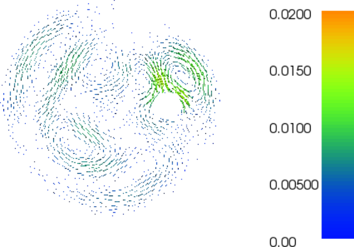
As can be seen in Figure 3 (left), the difference between the average EnB-POD and EnB-full velocities method appears to be quite small at T=5T=5. We can also see in Figure 4 that the energy and enstrophy of the EnB-POD method matches that of the EnB-full method when 66 POD basis vectors are used in the approximation. Lastly, it is seen in Table 1(a) that the L2 error of the approximation reduces monotonically as the number of POD basis functions used increases.
Refer to caption
Refer to caption
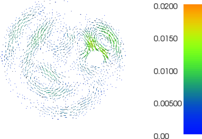
Figure 3. The difference between velocity field at the final time T=5T=5 of the EnB-full approximation and the En-POD approximation with 66 reduced basis vectors for example 1 (left) and example 2 (right).
Refer to caption
Refer to caption
Figure 4. For 0≤t≤50\leq t\leq 5, the energy (left) and enstrophy (right) of the ensemble determined for the EnB-full approximations and for the EnB-POD approximation of several dimensions for example 1.
(a) Example 1 (b) Example 2
RR error RR error
2 0.035785 2 0.035869
3 0.021379 3 0.021437
4 0.013802 4 0.013910
5 0.009067 5 0.009073
6 0.004886 6 0.004969
Table 1. The L2L^{2} relative error ‖uha​v​e−uRa​v​e‖2,0||u_{h}^{ave}-u_{R}^{ave}||_{2,0} vs. the dimension RR of the POD approximation for Examples 1 and 2.

6.2. Example 2

We next wish to test our reduced basis method in the extrapolatory setting, that is, for values of the perturbation parameter ϵ\epsilon different from those used to generate the reduced-order basis. To do so, we examine the problem used in Section 6.1 with the reduced basis for the EnB-POD approximation still generated by ϵ1=0.001\epsilon_{1}=0.001 and ϵ2=−0.001\epsilon_{2}=-0.001, but now we use five perturbations ϵ1=0.2\epsilon_{1}=0.2, ϵ2=0.4\epsilon_{2}=0.4, ϵ3=0.6\epsilon_{3}=0.6, ϵ4=0.8\epsilon_{4}=0.8, and ϵ5=1.0\epsilon_{5}=1.0 in the calculation of the EnB-full and EnB-POD solutions; all these values of ϵ\epsilon are well outside the interval [−0.001,0.001][-0.001,0.001].

The results for the ensemble average are given in Figures 3 (right), 5 and Table 1(b). We see that the results are identical to the first example except that, understandably, the relative error is slightly larger.

Refer to caption
Refer to caption
Figure 5. For 0≤t≤50\leq t\leq 5, the energy (left) and enstrophy (right) of the ensemble determined for the EnB-full approximations and for the EnB-POD approximation of several dimensions for example 2.

7. Conclusions

In this work, a second-order ensemble-POD method for the non-stationary Navier-Stokes equations is proposed and analyzed. This is an extension of the method first proposed in [6] and should prove useful in settings that require long-time integrations.

The method proposed in this work as well as in [6] only work well with low Reynolds number flows. Whereas there is a vast array of methods for the Navier-Stokes equations for high Reynolds number flows, within the POD/ensemble framework the literature is much more limited. A few recent works within this setting are the regularized reduced-order models developed in [21, 22, 23] and the regularized ensemble models in [14]. A natural extension of this work will be to incorporate these regularized methods into the ensemble-POD framework.

Acknowledgments

The authors gratefully acknowledge the support provided by the US Air Force Office of Scientific Research grant FA9550-15-1-0001 and US Department of Energy Office of Science grants DE-SC0009324 and DE-SC0010678.

References

  • [1] John Burkardt, Max Gunzburger, and Hyung-Chun Lee. Pod and cvt-based reduced-order modeling of navier–stokes flows. Computer Methods in Applied Mechanics and Engineering, 196(1):337–355, 2006.
  • [2] YT Feng, DRJ Owen, and D Perić. A block conjugate gradient method applied to linear systems with multiple right-hand sides. Computer methods in applied mechanics and engineering, 127(1):203–215, 1995.
  • [3] Roland W Freund and Manish Malhotra. A block qmr algorithm for non-hermitian linear systems with multiple right-hand sides. Linear Algebra and its Applications, 254(1):119–157, 1997.
  • [4] E Gallopulos and V Simoncini. Convergence of block gmres and matrix polynomials. Linear Algebra Appl, 247:97–119, 1996.
  • [5] Vivette Girault and Pierre-Arnaud Raviart. Finite element methods for Navier-Stokes equations: theory and algorithms, volume 5. Springer Science & Business Media, 2012.
  • [6] Max Gunzburger, Nan Jiang, and Michael Schneier. An ensemble-proper orthogonal decomposition method for the nonstationary navier–stokes equations. SIAM Journal on Numerical Analysis, 55(1):286–304, 2017.
  • [7] Max D Gunzburger. Finite Element Methods for Viscous Incompressible Flows: A guide to theory, practice, and algorithms. Elsevier, 2012.
  • [8] Max D Gunzburger, Janet S Peterson, and John N Shadid. Reduced-order modeling of time-dependent pdes with multiple parameters in the boundary data. Computer Methods in Applied Mechanics and Engineering, 196(4):1030–1047, 2007.
  • [9] Philip Holmes, John L Lumley, and Gal Berkooz. Turbulence, coherent structures, dynamical systems and symmetry. Cambridge university press, 1998.
  • [10] Traian Iliescu and Zhu Wang. Variational multiscale proper orthogonal decomposition: Navier-stokes equations. Numerical Methods for Partial Differential Equations, 30(2):641–663, 2014.
  • [11] Nan Jiang. A higher order ensemble simulation algorithm for fluid flows. Journal of Scientific Computing, pages 1–25, 2014.
  • [12] Nan Jiang. A second-order ensemble method based on a blended backward differentiation formula timestepping scheme for time-dependent navier?stokes equations. Numerical Methods for Partial Differential Equations, 33(1):34–61, 2017.
  • [13] Nan Jiang and William Layton. An algorithm for fast calculation of flow ensembles. International Journal for Uncertainty Quantification, 4(4), 2014.
  • [14] Nan Jiang and William Layton. Numerical analysis of two ensemble eddy viscosity numerical regularizations of fluid motion. Numerical Methods for Partial Differential Equations, 31(3):630–651, 2015.
  • [15] K. Kunisch and S. Volkwein. Galerkin proper orthogonal decomposition methods for a general equation in fluid dynamics. SIAM Journal on Numerical Analysis, 40(2):492–515, 2002.
  • [16] Karl Kunisch and Stefan Volkwein. Galerkin proper orthogonal decomposition methods for parabolic problems. Numerische mathematik, 90(1):117–148, 2001.
  • [17] O.A. Ladyzhenskai?a? The mathematical theory of viscous incompressible flow. Mathematics and its applications. Gordon and Breach, 1969.
  • [18] William Layton. Introduction to the numerical analysis of incompressible viscous flows, volume 6. Siam, 2008.
  • [19] Anders Logg, Kent-Andre Mardal, and Garth Wells. Automated solution of differential equations by the finite element method: The FEniCS book, volume 84. Springer Science & Business Media, 2012.
  • [20] Aziz Takhirov, Monika Neda, and Jiajia Waters. Time relaxation algorithm for flow ensembles. Numerical Methods for Partial Differential Equations, 32(3):757–777, 2016.
  • [21] D. Wells, Z. Wang, X. Xie, and T. Iliescu. An evolve-then-filter regularized reduced order model for convection-dominated flows. International Journal for Numerical Methods in Fluids, pages n/a–n/a, 2017. fld.4363.
  • [22] X. Xie, M. Mohebujjaman, L. G. Rebholz, and T. Iliescu. Data-Driven Filtered Reduced Order Modeling Of Fluid Flows. ArXiv e-prints, February 2017.
  • [23] X. Xie, D. Wells, Z. Wang, and T. Iliescu. Numerical Analysis of the Leray Reduced Order Model. ArXiv e-prints, February 2017.