A double-layer reduced model for fault flow on slipping domains with hybrid finite volume scheme

Alessio Fumagalli Isabelle Faille

Abstract

In this work we are interested in dealing with single-phase flows in fractured porous media for underground processes. We focus our attention on domains where the presence of faults, with thickness several orders of magnitude smaller than other characteristic sizes, can allow one part of the domain to slide past to the other. We propose a mathematical scheme where a reduced model for the fault flows is employed yielding a problem of co-dimension one. The hybrid finite volume method is used to obtain the discretized problem, which employs two different meshes for each fault, one associated with the porous-medium domain on each side of the fault. These two meshes can move with the corresponding domain, resulting in non-matching grids between the two parts of the fault. In an earlier paper a mathematical scheme was proposed where the numerical discretization considers the hybrid finite volume method. In this paper we focus on the well-posedness of the continuous problem, the convergence of the discretized problem, and with several numerical tests we support the theoretical findings.

keywords

Porous media, reduced model, faults, finite volume, non-matching grids

AMS

76S05, 65N08, 86A60

1 Introduction

Subsurface multi-phase flows in porous medium are strongly influenced by the presence of heterogeneities and in particular by the effect of faults, in which the flow can move differently in the surrounding medium both across and along the fault. Depending on the geophysical data, in particular the permeability, the faults can act as barriers or preferential paths for the flow. This behaviour is due to several factors: further fracturation of the fault zones, chemical reactions or generation at different geological times. The effect of the faults is extremely important for several applications, like fractured aquifers, $CO_{2}$ injection and sequestration or oil and gas reservoirs exploitation. See [9, 29, 25] for applications in real a context.

One of the most important aspects of faults is the difference between their characteristic sizes. We call the fault aperture the portion of rock containing the fault core and the surrounding damaged zone. Its typical thickness ranges from meters to a few tens of meters, while its length is generally of the same order as the size of the domain of interest. Normally the latter has extension of hundreds of kilo-meters with depth of tens of kilo-meters. Considering a conforming discretization of a real sedimentary basin with several faults, a standard numerical approximation can easily make the simulation unaffordable. Even if the literature on flows in fractured porous media is extensively developed, see for example [1, 10, 2], a general method is not yet available which can handle all the difficulties of this particular problem.

We focus our attention on the family of mathematical models which replace the fine description of the fault with an approximate one. The main idea of these models is to substitute the $N$ -dimensional description of the fault, in an $N$ -dimensional domain, by a new object of codimension one (an $N-1$ -dimensional object embedded in the $N$ -dimensional domain). New differential equations and suitable interface conditions are derived to couple the new problem. The firsts contributions were [4, 3], where a first reduced model (RM) is derived for only conductive faults, which cut entirely the domain. The fault mesh is composed of a set of contiguous edges of cells from the porous medium mesh, the method limits in this way the computational cost. Numerical experiments and theoretical results show the good behaviour of the proposed method. The authors in [17, 27, 6] consider a more general model where low permeable faults can also be taken into account. Finite element and finite volume approximations are considered with different numerical experiments. Three dimensional experiments, with realistic geometry and intersecting faults are presented in [5]. In the work [30] the authors consider a further generalization of the interface conditions, where different a-priori assumptions of fault pressure shapes in the normal direction are considered yielding a new RM with a model parameter. Theoretical analyses and numerical experiments show the robustness of the results in different situations. In this article we will refer to such a model as a single-layer reduced model (SLRM). The authors in [7] consider a partially immersed fault with new coupling conditions at the fault tips. Two-phase flow in porous media are considered in [28, 14] where a RM was introduced for this problem.

Based on the aforementioned mathematical model a different coupling approach was introduced in [12]. In this article the fault discretization is completely independent of the mesh of the porous medium. The extended finite element method (XFEM) is used to handle this geometrical non-conformity, yielding a very flexible tool for real simulations. Again with the same type of approximation we mention [23] for a description of convection and diffusion of a passive scalar in a porous media. In [22] the two-phase flow problem is considered with different approximation of the hyperbolic fluxes: upstream mobility and exact Riemann solver. In [20, 24] a general RM is presented for a network of faults where suitable interface conditions are considered in the intersecting regions.

Finally in [32, 18] the authors assume that one part of the domain can slip, because of the fault, with respect to another part. To handle this new feature, a new model is consider with a two layers approximation. In contrast to the SLRM, we will refer to the method proposed in [32] as a double-layer reduced model (DLRM) or simply (DL). Each part of the domain, situated along the fault, has its own fault approximation. Suitable interface conditions are considered for the layer-layer coupling.

In this work we continue the analyses of the mathematical scheme proposed in [18], where an approximation using the hybrid finite volume scheme [16] is considered for both the rock matrix, the fault, and their coupling. Furthermore the method can handle generic permeability fields as well as enforce local mass conservation for each cell. We present the DLRM, introducing its weak formulation and showing its well posedness. Numerical discretization with different theoretical results, including the convergence and model error, are presented in detail. A complex example with a sliding domain shows the effectiveness of the proposed approach also in such a situation.

This paper is organized as follow: in Section 2 the notations and the governing equations for the RM are presented as well as the analysis in the continuous spaces. Section 3 is devoted to the presentation of the discretization of the proposed schemes along with some important theoretical results. In Section 4 a collection of examples highlights the potential of the proposed methods. Finally, Section 5 contains the conclusions.

2 Mathematical problem

To ease the presentation we consider only one single fault that cuts entirely through the domain. The method can be generalized without any additional difficulties if we consider several non-intersecting faults.

2.1 Physical equations

Let us set, from now on, $i$ and $j$ indices with values $i\in\left\{1,2,f\right\}$ and $j\in\left\{1,2\right\}$ . We consider a regular domain $\Omega\subset\mathbb{R}^{N}$ , $N=2$ or 3, with Lipschitz-continuous boundary denoted by $\Gamma\vcentcolon=\overline{\Omega}\setminus\Omega$ . We suppose that $\Omega$ is divided into three disjoint subsets, such that $\overline{\Omega}=\cup_{i}\overline{\Omega_{i}}$ , where $\Omega_{f}$ represents the fault. Moreover the boundary is divided into $\Gamma_{i}\vcentcolon=\Gamma\cap\partial\Omega_{i}$ . Figure 1 shows an example.

Fig. 1: Representation of each sub-domain where the thickness of the fault is exaggerated for visualization purpose.

The interfaces, of codimension one, between the domain $\Omega_{j}$ and $\Omega_{f}$ are denoted as $\gamma_{j}\subset\mathbb{R}^{N}$ with unit normal $\bm{{n}}_{j}$ , pointing outwards from $\Omega_{j}$ . Since $\Omega_{1}$ can slide along $\Omega_{2}$ , or vice versa, due to the fault we subdivide the latter into two disjoint layers $\Omega_{f_{j}}$ , such that $\overline{\Omega_{f}}=\cup_{j}\overline{\Omega_{f_{j}}}$ , defined in the sequel. Then, following [30], we suppose that there exists a manifold ${\hat{\gamma}}\subset\mathbb{R}^{N}$ of co-dimension one and of class piecewise- $C^{2}$ such that $\hat{\gamma}$ represents the centre of the fault and $\Omega_{f}$ may be defined as

(1)

\displaystyle\Omega_{f_{j}}=\left\{\bm{{x}}\in\mathbb{R}^{N}:\bm{{x}}=\bm{{s}}+r\bm{{n}},\,\bm{{s}}\in{\hat{\gamma}},\,r\in T_{j}\right\}\quad\text{with}\quad T_{1}\vcentcolon=(-d/2,0),\,\,T_{2}\vcentcolon=(0,d/2).

In (1) we have denoted by $d\in C^{2}({\hat{\gamma}})$ the thickness of $\Omega_{f}$ and $\bm{{n}}$ the unit normal of ${\hat{\gamma}}$ , pointing from $\Omega_{1}$ to $\Omega_{2}$ . We assume that $|{\hat{\gamma}}|\gg d$ and there exist $c_{1},c_{2}\in\mathbb{R}^{+}$ , with $c_{2}$ “small”, such that $d\left(\bm{{s}}\right)>c_{1}$ and $|{d^{\prime}\left(\bm{{s}}\right)}|<c_{2}$ for all $\bm{{s}}\in{\hat{\gamma}}$ , i.e. the thickness of $\Omega_{f}$ is small and varies slowly compared to its other dimensions. Moreover we introduce the centre line ${\hat{\gamma}}_{j}$ of the fault layer $\Omega_{f_{j}}$ , translating ${\hat{\gamma}}$ to the middle of $T_{j}$ . We indicate with a lower case subscript the restriction of data and unknowns to the corresponding sub-domain of $\Omega$ . Finally we define the surrounding domain as $\overline{\Omega_{1,2}}\vcentcolon=\cup_{j}\overline{\Omega_{j}}$ and the fault centre line as $\overline{{\hat{\gamma}}_{1,2}}\vcentcolon=\cup_{j}\overline{{\hat{\gamma}}_{j}}$ .

We are interested in computing the steady pressure field $p$ and the velocity field, or Darcy velocity, $\bm{u}$ in the whole domain $\Omega$ , governed by the following Darcy problems, with the classical interface conditions, formulated in $\Omega_{i}$ . For simplicity we assume homogeneous boundary conditions for the pressure on $\Gamma$ . The problem is: find $(p,\bm{u})$ such that

(2)

\displaystyle\begin{aligned} &\!\!\!\begin{array}[]{ll}\nabla\cdot\bm{u}_{i}=q_{i}\\ \bm{u}_{i}+\Lambda_{i}\nabla p_{i}=\bm{{0}}\end{array}&&\text{in }\Omega_{i}\\ &p_{i}=0&&\text{on }\Gamma_{i}\end{aligned}\qquad\text{with}\qquad\begin{aligned} &p_{j}=p_{f}\\ &\bm{u}_{j}\cdot\bm{{n}}_{j}=\bm{u}_{f}\cdot\bm{{n}}_{j}\end{aligned}\text{ on }\gamma_{j}.

Here $\Lambda_{i}\in\left[L^{\infty}\left(\Omega_{i}\right)\right]^{N\times N}$ denotes the permeability tensor, such that for almost every $\bm{{x}}\in\Omega_{i}$ is symmetric and positive definite. More specifically we require that its eigenvalues are included in $0<\underline{\lambda}_{i}\leq\mathop{\rm eig}\Lambda_{i}\leq\overline{\lambda}_{i}$ , with $\underline{\lambda}_{i},\overline{\lambda}_{i}\in\mathbb{R}^{+}$ . In (2) $q_{i}\in L^{2}\left(\Omega_{i}\right)$ is a scalar source term which may represents a possible volume source or sink.

We have the following standard result for the Darcy problem, see [11, 31, 15].

Theorem 1.

Under the given hypothesis on the data, problem (2) is well posed. In particular, we have $\left(\bm{u},p\right)\in{\bm{H}}_{\rm div}\left(\Omega\right)\times L^{2}\left(\Omega\right)$ .

2.2 The reduced model

For readers convenience we recall the main results and a brief derivation of the DLRM, a more detailed derivation can be found in [32, 18]. We introduce the projection matrices in the normal and tangential directions of ${\hat{\gamma}}$ as $\bm{{N}}\vcentcolon=\bm{{n}}\otimes\bm{{n}}$ and $\bm{{T}}\vcentcolon=\bm{{I}}-\bm{{N}}$ , respectively. The Darcy velocity in the fault can be decomposed into its normal and tangential parts as $\bm{u}_{f}=\bm{{N}}\bm{u}_{f}+\bm{{T}}\bm{u}_{f}=\bm{u}_{f,\bm{{n}}}+\bm{u}_{f,\bm{{\tau}}}$ , with $\bm{u}_{f,\bm{{n}}}\vcentcolon=\bm{{N}}\bm{u}_{f}$ and $\bm{u}_{f,\bm{{\tau}}}\vcentcolon=\bm{{T}}\bm{u}_{f}$ . Moreover we introduce also the normal and tangential divergence and gradient on ${\hat{\gamma}}$ , given $\bm{v}$ and $v$ two regular functions we define

	$\displaystyle\nabla\cdot\bm{v}=\nabla_{\bm{{n}}}\cdot\bm{v}+\nabla_{\bm{{\tau}}}\cdot\bm{v}\quad\text{with}\quad\nabla_{\bm{{n}}}\cdot\bm{v}\vcentcolon=\bm{{N}}:\nabla\bm{v}\quad\text{and}\quad\nabla_{\bm{{\tau}}}\cdot\bm{v}\vcentcolon=\bm{{T}}:\nabla\bm{v},$
	$\displaystyle\nabla v=\nabla_{\bm{{n}}}v+\nabla_{\bm{{\tau}}}v\quad\text{with}\quad\nabla_{\bm{{n}}}v\vcentcolon=\bm{{N}}\nabla v\quad\text{and}\quad\nabla_{\bm{{\tau}}}v\vcentcolon=\bm{{T}}\nabla v.$

The conservation equation, for each side of the fault, is integrated along its normal direction on $T_{j}$ to obtain a conservation equation written in the tangential space of $\gamma_{j}$

(3)

\displaystyle\nabla_{\bm{{\tau}}}\cdot\hat{\bm{u}}_{j}=\hat{q}_{j}+\left\llbracket{\bm{u}\cdot\bm{{n}}}\right\rrbracket_{\gamma_{j}}\quad\text{in }{\hat{\gamma}}_{j}.

In the latter equation we have indicated with $\hat{\bm{u}}_{j}$ the reduced flux for each layer of the fault, defined as $\hat{\bm{u}}_{j}\vcentcolon=\int_{T_{j}}\bm{u}_{f,\bm{{\tau}}}$ , and the reduced source term as $\hat{q}_{j}\vcentcolon=\int_{T_{j}}q_{f}$ . Moreover $\left\llbracket{\bm{u}\cdot\bm{{n}}}\right\rrbracket_{\gamma_{j}}$ indicates the jump of the flux across the corresponding layer of the fault, defined as

\displaystyle\left\llbracket{\bm{u}\cdot\bm{{n}}}\right\rrbracket_{\gamma_{j}}\vcentcolon=(-1)^{j}(\left.\bm{u}_{f}\cdot\bm{{n}}\right|_{\hat{\gamma}}-\left.\bm{u}_{f}\cdot\bm{{n}}\right|_{\gamma_{j}})=(-1)^{j}\left(\left.\hat{u}_{\bm{{n}}}-\bm{u}_{j}\cdot\bm{{n}}\right|_{\gamma_{j}}\right),

where $\hat{u}_{\bm{{n}}}$ stands for $\left.\bm{u}_{f}\cdot\bm{{n}}\right|_{\hat{\gamma}}$ . The Darcy equation require that the permeability in the fault can be written as $\Lambda_{f}=\lambda_{f,\bm{{n}}}\bm{{N}}+\lambda_{f,\bm{{\tau}}}\bm{{T}}$ , with $\lambda_{f,\bm{{n}}}$ and $\lambda_{f,\bm{{\tau}}}$ strictly positive for almost every $\bm{{x}}\in\Omega_{f}$ . For a more general case refer to [7]. Considering the projected Darcy equation on the tangential space of ${\hat{\gamma}}_{j}$ , integrated in the normal direction of the latter, we obtain

(4)

\displaystyle\hat{\bm{u}}_{j}+\hat{\lambda}\nabla_{\bm{{\tau}}}\hat{p}_{j}=\bm{{0}}\quad\text{in }{\hat{\gamma}}_{j},

where $\hat{p}_{j}$ is the reduced pressure in each part of the fault, defined as $\hat{p}_{j}\vcentcolon=\frac{2}{d}\int_{T_{j}}p_{f}$ , and $\hat{\lambda}$ is the effective permeability in the tangential direction, defined as $\hat{\lambda}\vcentcolon=d\lambda_{f,\bm{{\tau}}}/2$ . We can consider a different value of $\hat{\lambda}$ for each layer but, for easy of the presentation, we avoid to specify it. In Section 4.4 we present an example with different value of $\hat{\lambda}$ for each layer of the fault. Projecting the Darcy equation on the normal space of the fault and integrating in the normal direction on the first half of $T_{1}$ , and on the second half of $T_{2}$ respectively, we end up with the coupling conditions

\displaystyle\bm{u}_{1}\cdot\bm{{n}}=2\lambda_{\hat{\gamma}}\left(p_{1}-\hat{p}_{1}\right)\quad\text{and}\quad\bm{u}_{2}\cdot\bm{{n}}=2\lambda_{\hat{\gamma}}\left(\hat{p}_{2}-p_{2}\right)

where $\lambda_{\hat{\gamma}}$ is the effective permeability in the normal direction of the fault, defined as $\lambda_{\hat{\gamma}}\vcentcolon=2\lambda_{f,\bm{{n}}}/d$ . In the latter equations we have used a suitable approximation of the integral of $\bm{u}_{i}\cdot\bm{{n}}$ . We need to introduce an additional equation to express the coupling of the velocity between the two sides of the fault. We consider again the projection of the Darcy equation on the normal space of ${\hat{\gamma}}$ and integrating, in the normal direction, between the second half of $T_{1}$ and the first half of $T_{2}$ we obtain

(5)

\displaystyle\hat{u}_{\bm{{n}}}=\lambda_{\hat{\gamma}}\left\llbracket{\hat{p}}\right\rrbracket_{{\hat{\gamma}}},

where, in this case, the jump operator is defined as $\left\llbracket{\hat{p}}\right\rrbracket_{{\hat{\gamma}}}\vcentcolon=\hat{p}_{1}-\hat{p}_{2}$ . Considering (2) for $i=j$ coupled with (3), (4), (2.2) and (5) we end up with the following problem: find $(\bm{u}_{j},p_{j})$ and $(\hat{\bm{u}}_{j},\hat{p}_{j})$ such that


(6a)		$\displaystyle\begin{aligned} &\!\!\!\begin{array}[]{ll}\nabla\cdot\bm{u}_{i}=q_{i}\\ \bm{u}_{i}+\Lambda_{i}\nabla p_{i}=\bm{{0}}\end{array}&&\text{in }\Omega_{i}\\ &p_{i}=0&&\text{on }\Gamma_{i}\end{aligned}\qquad\text{and}\qquad\begin{aligned} &\!\!\!\begin{array}[]{ll}\nabla_{\bm{{\tau}}}\cdot\hat{\bm{u}}_{j}=\hat{q}_{j}+\left\llbracket{\bm{u}\cdot\bm{{n}}}\right\rrbracket_{\gamma_{j}}\\ \hat{\bm{u}}_{j}+\hat{\lambda}\nabla_{\bm{{\tau}}}\hat{p}_{j}=\bm{{0}}\end{array}&&\text{in }{\hat{\gamma}}_{j}\\ &\hat{p}_{j}=0&&\text{on }\partial{\hat{\gamma}}_{j},\end{aligned}$
with the coupling conditions

(6b)		$\displaystyle\begin{aligned} &\bm{u}_{1}\cdot\bm{{n}}=2\lambda_{\hat{\gamma}}\left(p_{1}-\hat{p}_{1}\right)&\quad&\text{on }{\hat{\gamma}}_{1}\\ &\bm{u}_{2}\cdot\bm{{n}}=2\lambda_{\hat{\gamma}}\left(\hat{p}_{2}-p_{2}\right)&&\text{on }{\hat{\gamma}}_{2}\\ &\hat{u}_{\bm{{n}}}=\lambda_{\hat{\gamma}}\left\llbracket{\hat{p}}\right\rrbracket_{{\hat{\gamma}}}&&\text{on }{\hat{\gamma}}\end{aligned}$

Summing and subtracting the first two equations of (6b) we end up with an equivalent set of coupling conditions

(6b-bis)

\displaystyle\begin{aligned} &\left\{\!\!\left\{{\bm{u}\cdot\bm{{n}}}\right\}\!\!\right\}_{{\hat{\gamma}}}=\lambda_{\hat{\gamma}}\left(\left\llbracket{p}\right\rrbracket_{{\hat{\gamma}}}-\left\llbracket{\hat{p}}\right\rrbracket_{{\hat{\gamma}}}\right)\\ &\left\llbracket{\bm{u}\cdot\bm{{n}}}\right\rrbracket_{{\hat{\gamma}}}=4\lambda_{\hat{\gamma}}\left(\left\{\!\!\left\{{p}\right\}\!\!\right\}_{{\hat{\gamma}}}-\left\{\!\!\left\{{\hat{p}}\right\}\!\!\right\}_{{\hat{\gamma}}}\right)\\ &\hat{u}_{\bm{{n}}}=\lambda_{\hat{\gamma}}\left\llbracket{\hat{p}}\right\rrbracket_{{\hat{\gamma}}}\end{aligned}\quad\text{on }{\hat{\gamma}},

where we have indicated by $\left\{\!\!\left\{{\hat{p}}\right\}\!\!\right\}_{{\hat{\gamma}}}\vcentcolon=\frac{1}{2}\left(\hat{p}_{1}-\hat{p}_{2}\right)$ and, with an abuse of notations, by $\left\{\!\!\left\{{\bm{u}\cdot\bm{{n}}}\right\}\!\!\right\}_{{\hat{\gamma}}}\vcentcolon=\frac{1}{2}\left(\bm{u}_{1}\cdot\bm{{n}}+\bm{u}_{2}\cdot\bm{{n}}\right)$ , $\left\llbracket{\bm{u}\cdot\bm{{n}}}\right\rrbracket_{{\hat{\gamma}}}\vcentcolon=\left(\bm{u}_{1}\cdot\bm{{n}}-\bm{u}_{2}\cdot\bm{{n}}\right)$ , $\left\llbracket{p}\right\rrbracket_{{\hat{\gamma}}}\vcentcolon=p_{1}-p_{2}$ and $\left\{\!\!\left\{{p}\right\}\!\!\right\}_{{\hat{\gamma}}}\vcentcolon=\frac{1}{2}\left(p_{1}+p_{2}\right)$ .

Remark 1.

In the sequel we will use a numerical scheme based on the primal formulation of (6), since it is a trivial derivation we will refer to this problem for both its dual or primal formulation.

2.3 Weak formulation

In the sequel we will use the symbols $a\lesssim b\Leftrightarrow a\leq c_{1}b$ and $a\gtrsim b\Leftrightarrow a\geq c_{2}b$ for some $c_{1},c_{2}\in\mathbb{R}^{+}$ dependent only on the data problem of (6) or on data which are not important for the analyses. The constants are independent from the grid size. First of all we introduce the functional setting for problem (6). We consider the functional spaces ${\mathcal{V}}_{j}\vcentcolon=H_{\Gamma_{j}}^{1}\left(\Omega_{j}\right)$ , endowed with the usual norms, and the global functional space for the domain ${\mathcal{V}}\vcentcolon=\prod_{j}{\mathcal{V}}_{j}$ . Moreover we define

\displaystyle\hat{{\mathcal{V}}}_{j}\vcentcolon=\left\{\hat{v}_{j}:\,\hat{v}_{j}|_{\partial{\hat{\gamma}}_{j}}=0,\hat{v}_{j}\in L^{2}\left({\hat{\gamma}}_{j}\right)\text{ and }\nabla_{\bm{{\tau}}}\hat{v}_{j}\in\left[L^{2}\left({\hat{\gamma}}_{j}\right)\right]^{N-1}\right\}\quad\text{and}\quad\hat{{\mathcal{V}}}\vcentcolon=\prod_{j}\hat{{\mathcal{V}}}_{j},

with norms

	$\displaystyle{\\|{\hat{v}_{j}}\\|}_{\hat{{\mathcal{V}}}_{j}}^{2}\vcentcolon={\\|{\hat{v}_{j}}\\|}_{L^{2}({\hat{\gamma}}_{j})}^{2}+{\\|{\nabla_{\bm{{\tau}}}\hat{v}_{j}}\\|}_{L^{2}({\hat{\gamma}}_{j})}^{2},\quad{\\|{v}\\|}_{{\mathcal{V}}}^{2}\vcentcolon=\sum_{j}{\\|{v}\\|}_{{\mathcal{V}}_{j}}^{2},$
	$\displaystyle{\\|{\hat{v}}\\|}_{\hat{{\mathcal{V}}}}^{2}\vcentcolon=\sum_{j}{\\|{\hat{v}_{j}}\\|}_{\hat{{\mathcal{V}}}_{j}}^{2}\quad\text{and}\quad{\\|{\left(v,\hat{v}\right)}\\|}_{{\mathcal{V}}\times\hat{{\mathcal{V}}}}^{2}\vcentcolon={\\|{v}\\|}_{{\mathcal{V}}}^{2}+{\\|{\hat{v}}\\|}_{\hat{{\mathcal{V}}}}^{2}$

Considering $\left(\cdot,\cdot\right)_{A}:L^{2}(A)\times L^{2}(A)\rightarrow\mathbb{R}$ the scalar product in $L^{2}(A)$ , with $A\subset\Omega$ , we introduce the bilinear forms for the diffusive parts as

	$\displaystyle a_{\Omega}\left(p,v\right)\vcentcolon=\sum_{j}\left(\Lambda_{j}\nabla p_{j},\nabla v_{j}\right)_{\Omega_{j}}\quad\text{and}\quad a_{\hat{\gamma}}\left(\hat{p},\hat{v}\right)\vcentcolon=\sum_{j}\left(\hat{\lambda}\nabla_{\bm{{\tau}}}\hat{p}_{j},\nabla_{\bm{{\tau}}}\hat{v}_{j}\right)_{{\hat{\gamma}}_{j}},$
	$\displaystyle a\left(\left(p,\hat{p}\right),\left(v,\hat{v}\right)\right)\vcentcolon=a_{\Omega}\left(p,v\right)+a_{\hat{\gamma}}\left(\hat{p},\hat{v}\right).$

Moreover we consider also the bilinear forms for the coupling conditions, considering (-bis), for the jumps and averages as

	$\displaystyle av\big({\left(p,\hat{p}\right)},{\left(v,\hat{v}\right)}\big)\vcentcolon=4\left(\lambda_{\hat{\gamma}}\left\{\!\!\left\{{p}\right\}\!\!\right\}_{{\hat{\gamma}}}-\lambda_{\hat{\gamma}}\left\{\!\!\left\{{\hat{p}}\right\}\!\!\right\}_{{\hat{\gamma}}},\left\{\!\!\left\{{v}\right\}\!\!\right\}_{{\hat{\gamma}}}-\left\{\!\!\left\{{\hat{v}}\right\}\!\!\right\}_{{\hat{\gamma}}}\right)_{\hat{\gamma}},$
	$\displaystyle j\big({\left(p,\hat{p}\right)},{\left(v,\hat{v}\right)}\big)\vcentcolon=\left(\lambda_{\hat{\gamma}}\left\llbracket{p}\right\rrbracket_{{\hat{\gamma}}}-\lambda_{\hat{\gamma}}\left\llbracket{\hat{p}}\right\rrbracket_{{\hat{\gamma}}},\left\llbracket{v}\right\rrbracket_{{\hat{\gamma}}}-\left\llbracket{\hat{v}}\right\rrbracket_{{\hat{\gamma}}}\right)_{\hat{\gamma}}+\left(\lambda_{\hat{\gamma}}\left\llbracket{\hat{p}}\right\rrbracket_{{\hat{\gamma}}},\left\llbracket{\hat{v}}\right\rrbracket_{{\hat{\gamma}}}\right)_{\hat{\gamma}},$
	$\displaystyle cc\big({\left(p,\hat{p}\right)},{\left(v,\hat{v}\right)}\big)\vcentcolon=av\big({\left(p,\hat{p}\right)},{\left(v,\hat{v}\right)}\big)+j\big({\left(p,\hat{p}\right)},{\left(v,\hat{v}\right)}\big)$

or considering the equivalent form (6b) we introduce

	$\displaystyle cc\big({\left(p,\hat{p}\right)},{\left(v,\hat{v}\right)}\big)\vcentcolon=2\left(\lambda_{\hat{\gamma}}p_{1}-\lambda_{\hat{\gamma}}\hat{p}_{1},v_{1}-\hat{v}_{1}\right)_{{\hat{\gamma}}_{1}}+2\left(\lambda_{\hat{\gamma}}p_{2}-\lambda_{\hat{\gamma}}\hat{p}_{2},v_{2}-\hat{v}_{2}\right)_{{\hat{\gamma}}_{2}}+$
	$\displaystyle+\left(\lambda_{\hat{\gamma}}\left\llbracket{\hat{p}}\right\rrbracket_{{\hat{\gamma}}},\left\llbracket{\hat{v}}\right\rrbracket_{{\hat{\gamma}}}\right)_{{\hat{\gamma}}}.$

The global bilinear form is defined as

\displaystyle A{\left({\left(p,\hat{p}\right)},{\left(v,\hat{v}\right)}\right)}\vcentcolon=a\big({\left(p,\hat{p}\right)},{\left(v,\hat{v}\right)}\big)+cc\big({\left(p,\hat{p}\right)},{\left(v,\hat{v}\right)}\big).

Finally we introduce the functional for the right-hand side

\displaystyle F\left(v,\hat{v}\right)\vcentcolon=\sum_{j}\left(q_{j},v_{j}\right)_{\Omega_{j}}+\left(\hat{q}_{j},\hat{v}_{j}\right)_{{\hat{\gamma}}_{j}}.

We present the weak formulation for problem (6): find $\left(p,\hat{p}\right)\in{\mathcal{V}}\times\hat{{\mathcal{V}}}$ such that

(7)

\displaystyle A{\left({\left(p,\hat{p}\right)},{\left(v,\hat{v}\right)}\right)}=F\left(v,\hat{v}\right)\qquad\forall\left(v,\hat{v}\right)\in{\mathcal{V}}\times\hat{{\mathcal{V}}}.

Lemma 2 (Well posedness).

Problem 7 is well posed, moreover ${\|{\left(p,\hat{p}\right)}\|}_{{\mathcal{V}}\times\hat{{\mathcal{V}}}}\lesssim 1$ .

Proof.

Clearly all the bilinear forms and the functional introduced are linear, we are going to apply the Lax-Milgram theorem and obtain the existence and uniqueness of the solution. We prove the continuity of the bilinear forms, introducing $c_{0}=\displaystyle\max_{i=1,2}{\|{\Lambda_{i}}\|}_{L^{\infty}(\Omega_{i})}$ , we have

\displaystyle|{a\big({\left(p,\hat{p}\right)},{\left(v,\hat{v}\right)}\big)}|\leq|{a_{\Omega}\left(p,v\right)}|+|{a_{\hat{\gamma}}\left(\hat{p},\hat{v}\right)}|\leq c_{0}{\|{p}\|}_{{\mathcal{V}}}{\|{v}\|}_{{\mathcal{V}}}+{\|{\hat{\lambda}}\|}_{L^{\infty}({\hat{\gamma}})}{\|{\hat{p}}\|}_{\hat{{\mathcal{V}}}}{\|{\hat{v}}\|}_{\hat{{\mathcal{V}}}},

considering the maximum between $c_{0}$ and the norm of $\hat{\lambda}$ we obtain the bound for the bilinear form: $|{a\big({\left(p,\hat{p}\right)},{\left(v,\hat{v}\right)}\big)}|\lesssim{\|{\left(p,\hat{p}\right)}\|}_{{\mathcal{V}}\times\hat{{\mathcal{V}}}}{\|{\left(v,\hat{v}\right)}\|}_{{\mathcal{V}}\times\hat{{\mathcal{V}}}}$ . We consider now the bilinear forms associated to the coupling conditions

\displaystyle|{cc\big({\left(p,\hat{p}\right)},{\left(v,\hat{v}\right)}\big)}|\leq|{av\big({\left(p,\hat{p}\right)},{\left(v,\hat{v}\right)}\big)}|+|{j\big({\left(p,\hat{p}\right)},{\left(v,\hat{v}\right)}\big)}|,

using the inequality for the averages and the jumps operators introduced in [6], i.e.

\displaystyle{\|{\left\{\!\!\left\{{v}\right\}\!\!\right\}_{{\hat{\gamma}}}}\|}_{L^{2}({\hat{\gamma}})}\lesssim{\|{v}\|}_{{\mathcal{V}}}\quad\text{and}\quad{\|{\left\llbracket{v}\right\rrbracket_{{\hat{\gamma}}}}\|}_{L^{2}({\hat{\gamma}})}\lesssim{\|{v}\|}_{{\mathcal{V}}},

then we have

	$\displaystyle\|{av\big({\left(p,\hat{p}\right)},{\left(v,\hat{v}\right)}\big)}\|\lesssim\|{\left(\left\{\!\!\left\{{p}\right\}\!\!\right\}_{{\hat{\gamma}}}-\left\{\!\!\left\{{\hat{p}}\right\}\!\!\right\}_{{\hat{\gamma}}},\left\{\!\!\left\{{v}\right\}\!\!\right\}_{{\hat{\gamma}}}-\left\{\!\!\left\{{\hat{v}}\right\}\!\!\right\}_{{\hat{\gamma}}}\right)_{\hat{\gamma}}}\|\lesssim{\\|{\left(p,\hat{p}\right)}\\|}_{{\mathcal{V}}\times\hat{{\mathcal{V}}}}{\\|{\left(v,\hat{v}\right)}\\|}_{{\mathcal{V}}\times\hat{{\mathcal{V}}}},$
	$\displaystyle\|{j\big({\left(p,\hat{p}\right)},{\left(v,\hat{v}\right)}\big)}\|\lesssim\|{\left(\left\llbracket{p}\right\rrbracket_{{\hat{\gamma}}}-\left\llbracket{\hat{p}}\right\rrbracket_{{\hat{\gamma}}},\left\llbracket{v}\right\rrbracket_{{\hat{\gamma}}}-\left\llbracket{\hat{v}}\right\rrbracket_{{\hat{\gamma}}}\right)_{\hat{\gamma}}}\|+\|{\left(\left\llbracket{\hat{p}}\right\rrbracket_{{\hat{\gamma}}},\left\llbracket{\hat{v}}\right\rrbracket_{{\hat{\gamma}}}\right)_{\hat{\gamma}}}\|\lesssim{\\|{\left(p,\hat{p}\right)}\\|}_{{\mathcal{V}}\times\hat{{\mathcal{V}}}}{\\|{\left(v,\hat{v}\right)}\\|}_{{\mathcal{V}}\times\hat{{\mathcal{V}}}}$

The functional in (7) is clearly continuous, while the coercivity of the global bilinear form is proved given the positivity of $cc\big({\cdot},{\cdot}\big)$ and the coercivity of the stiffness bilinear form. The bound on the solution is obtained considering the coercivity of $a$ and the continuity of $F$ . ∎

3 Numerical approximation

We introduce the definition of discretization for $\Omega_{1,2}$ , the porous medium domain. The discretization of the fault follows from the discretization of the domain. We report in Figure 2 a schematic representation of some notations we introduce in Definition 3.

Fig. 2: Notation useful for the numerical scheme, given a cell

K

Definition 3 (Discretization of $\Omega_{1,2}$ ).

A discretization of $\Omega_{1,2}$ , denoted by ${\mathcal{D}}$ , is defined as the triplet ${\mathcal{D}}\vcentcolon=(\mathcal{M},\mathcal{E},\mathcal{P})$ where

•

$\mathcal{M}$ is the set of control volumes. The control volumes are non-empty connected and disjoint subset of $\Omega_{1,2}$ such that $\overline{\Omega_{1,2}}=\cup_{K\in\mathcal{M}}\overline{K}$ . Let $|{K}|>0$ the measure of $K$ and $h_{K}\in\mathbb{R}^{+}$ its diameter. We indicate by $\displaystyle h_{\mathcal{D}}\vcentcolon=\sup\left\{h_{K},K\in\mathcal{M}\right\}$ the diameter of the discretization;
•

$\mathcal{E}$ is the set of the edges, divided into the set of external edges $\mathcal{E}_{\rm ext}=\partial\Omega$ , the set of internal edges $\mathcal{E}_{\rm int}$ and the set of fault edges $\mathcal{E}_{\gamma}=\partial\Omega_{1}\cap\partial\Omega_{2}$ ; we have $\mathcal{E}=\mathcal{E}_{\rm int}\cup\mathcal{E}_{\rm ext}\cup\mathcal{E}_{\gamma}$ . Let $|{\sigma}|>0$ the measure of $\sigma$ . We denote by $\mathcal{E}_{K}\subset\mathcal{E}$ the set of all edges of a control volume $K$ and by $\mathcal{M}_{\sigma}\vcentcolon=\left\{K\in\mathcal{M}:\,\sigma\in\mathcal{E}_{K}\right\}$ the set of all elements facing a given edge $\sigma$ ;
•

$\mathcal{P}$ is the set of points, defined by $\mathcal{P}\vcentcolon=\left(\bm{{x}}_{K}\right)_{K\in\mathcal{M}}\cup\left(\bm{{x}}_{\sigma}\right)_{\sigma\in\mathcal{M}}$ , where $\bm{x}_{K}$ is the centre of mass for the cell $K\in\mathcal{M}$ and $\bm{x}_{\sigma}$ is the barycentre of the face $\sigma\in\mathcal{E}$ ;
•

for any cell $K\in\mathcal{M}$ and face $\sigma\in\mathcal{E}_{K}$ we indicate by $\bm{{n}}_{K,\sigma}$ the unit vector normal to $\sigma$ outward to $K$ ;
•

$D_{K,\sigma}\in K$ is the cone with vertex $\bm{{x}}_{K}$ and basis $\sigma\in\mathcal{E}_{K}$ . We indicate with $d_{K,\sigma}\in\mathbb{R}^{+}$ the orthogonal distance between $\bm{x}_{K}$ and $\sigma$ .

The set, or family, of all the discretizations ${\mathcal{D}}$ is denoted by ${\mathcal{F}}$ .

We introduce also a parameter that measure the quality of the mesh

(8)

\displaystyle\theta_{\mathcal{D}}\vcentcolon=\max\left(\max_{\sigma\in\mathcal{E}_{\rm int},\mathcal{M}_{\sigma}=\left\{K,L\right\}}\dfrac{d_{K,\sigma}}{d_{L,\sigma}},\max_{K\in\mathcal{M},\sigma\in\mathcal{E}_{K}}\dfrac{h_{K}}{d_{K,\sigma}}\right)

For the discretization of the fault, in problem (6), we suppose that ${\mathcal{D}}$ is conforming with the fault, i.e. the fault is represented by a set of continuous edges of $\mathcal{E}_{\gamma}$ . However we allow a non-matching approximation of ${\hat{\gamma}}_{1}$ and ${\hat{\gamma}}_{2}$ . We indicate with $\hat{{\mathcal{D}}}=\left(\hat{\mathcal{M}},\hat{\mathcal{E}},\hat{\mathcal{P}}\right)\in\hat{{\mathcal{F}}}$ the discretization of the fault, where $\hat{\mathcal{M}}$ is the set of control volumes of the approximation of ${\hat{\gamma}}_{1,2}$ . We consider the same notation of Definition 3 where $\hat{{\mathcal{F}}}$ is considered instead of ${\mathcal{F}}$ . Thanks to Definition 3 we have $\bm{{n}}_{K,\sigma}=-\bm{{n}}_{L,\sigma}$ for each $\mathcal{M}_{\sigma}=\left\{K,L\right\}$ , while for the fault we assume the following statement.

Hypotheses 1 (Normal discrepancy).

For each $\sigma\in\hat{\mathcal{E}}$ , with $\mathcal{M}_{\sigma}=\left\{K,L\right\}$ , we suppose that

\displaystyle\bm{{n}}_{K,\sigma}+\bm{{n}}_{L,\sigma}=\mathcal{O}\left(h_{\mathcal{D}}\right)\quad\text{as}\quad h_{\mathcal{D}}\rightarrow 0.

We consider also the mesh quality parameter $\theta_{\hat{{\mathcal{D}}}}$ for $\hat{{\mathcal{D}}}$ , defined as (8) where $\hat{\mathcal{M}}$ and $\hat{\mathcal{E}}_{\rm int}$ are used instead of $\mathcal{M}$ and $\mathcal{E}_{\rm int}$ , respectively. We assume that exists $\theta\in\mathbb{R}^{+}$ such that

\displaystyle\theta\vcentcolon=\max\left\{\sup\left\{\theta_{\mathcal{D}},{\mathcal{D}}\in{\mathcal{F}}\right\},\sup\left\{\theta_{\hat{{\mathcal{D}}}},\hat{{\mathcal{D}}}\in\hat{{\mathcal{F}}}\right\}\right\}.

We introduce the following discrete spaces for both the domain and the fault discretization: one degree of freedom for each element and one for each face, namely for the porous domain

\displaystyle{\mathcal{V}}_{{\mathcal{D}}}\vcentcolon=\left\{v=\left(\left(v_{K}\right)_{K\in\mathcal{M}},\left(v_{\sigma}\right)_{\sigma\in\mathcal{E}}\right):v_{K}\in\mathbb{R},v_{\sigma}\in\mathbb{R}\right\}\text{ and }{\mathcal{V}}_{{\mathcal{D}},0}\vcentcolon=\left\{v\in{\mathcal{V}}_{{\mathcal{D}}}:v_{\sigma}=0\forall\sigma\in\mathcal{E}_{\rm ext}\right\},

and for the fault

\displaystyle\hat{{\mathcal{V}}}_{{\mathcal{D}}}\vcentcolon=\left\{\hat{v}=\left(\left(\hat{v}_{K}\right)_{K\in\hat{\mathcal{M}}},\left(\hat{v}_{\sigma}\right)_{\sigma\in\hat{\mathcal{E}}}\right):\hat{v}_{K}\in\mathbb{R},\hat{v}_{\sigma}\in\mathbb{R}\right\}\text{ and }\hat{{\mathcal{V}}}_{{\mathcal{D}},0}\vcentcolon=\left\{\hat{v}\in\hat{{\mathcal{V}}}_{{\mathcal{D}}}:\hat{v}_{\sigma}=0\forall\sigma\in\hat{\mathcal{E}}_{\rm ext}\right\}.

Where the spaces ${\mathcal{V}}_{{\mathcal{D}},0}\subset{\mathcal{V}}_{{\mathcal{D}}}$ and $\hat{{\mathcal{V}}}_{{\mathcal{D}},0}\subset\hat{{\mathcal{V}}}_{{\mathcal{D}}}$ include the boundary conditions. We consider also the global discrete space as ${\mathcal{Y}}_{{\mathcal{D}}}\vcentcolon={\mathcal{V}}_{{\mathcal{D}}}\times\hat{{\mathcal{V}}}_{{\mathcal{D}}}$ and ${\mathcal{Y}}_{{\mathcal{D}},0}\vcentcolon={\mathcal{V}}_{{\mathcal{D}},0}\times\hat{{\mathcal{V}}}_{{\mathcal{D}},0}$ , with ${\mathcal{Y}}_{{\mathcal{D}},0}\subset{\mathcal{Y}}_{{\mathcal{D}}}$ . Since the discretization of the fault is constructed from the discretization of the porous medium, for exigence in notation we will indicate, in presence of both, only the latter. The spaces ${\mathcal{V}}_{{\mathcal{D}},0}$ and $\hat{{\mathcal{V}}}_{{\mathcal{D}},0}$ are the discrete approximations of ${\mathcal{V}}$ and $\hat{{\mathcal{V}}}$ , respectively. For each of the previous space we introduce a discrete semi-norm: given $v\in{\mathcal{V}}_{{\mathcal{D}}}$ and $\hat{v}\in\hat{{\mathcal{V}}}_{{\mathcal{D}}}$ , we define

(9)

\displaystyle|{v}|_{{\mathcal{V}}_{{\mathcal{D}}}}\vcentcolon=\sum_{K\in\mathcal{M}}\sum_{\sigma\in\mathcal{E}_{K}}\dfrac{|{\sigma}|}{d_{K,\sigma}}\left(v_{\sigma}-v_{K}\right)^{2},\quad|{\hat{v}}|_{\hat{{\mathcal{V}}}_{{\mathcal{D}}}}\vcentcolon=\sum_{K\in\hat{\mathcal{M}}}\sum_{\sigma\in\mathcal{E}_{K}}\dfrac{|{\sigma}|}{d_{K,\sigma}}\left(\hat{v}_{\sigma}-\hat{v}_{K}\right)^{2}

and concerning the global space for all $\left(v,\hat{v}\right)\in{\mathcal{Y}}_{{\mathcal{D}}}$ we have $|{\left(v,\hat{v}\right)}|_{{\mathcal{Y}}_{{\mathcal{D}}}}^{2}\vcentcolon=|{v}|_{{\mathcal{V}}_{{\mathcal{D}}}}^{2}+|{\hat{v}}|_{\hat{{\mathcal{V}}}_{{\mathcal{D}}}}^{2}$ . Given a function $v\in{\mathcal{V}}_{{\mathcal{D}}}$ , let us set $\Pi_{\mathcal{M}}v\in L^{2}(\Omega)$ the piece-wise function defined by $\Pi_{\mathcal{M}}v(\bm{{x}})=v_{K}$ for a.e. $\bm{{x}}\in K$ , for all $K\in\mathcal{M}$ . We indicate with $\Pi_{\hat{\mathcal{M}}}:\hat{{\mathcal{V}}}_{{\mathcal{D}}}\rightarrow L^{2}({\hat{\gamma}}_{1,2})$ the same projector operator defined on the two layers of the fault. Introducing $D_{\sigma}v\vcentcolon=|{v_{K}-v_{L}}|$ and $d_{\sigma}\vcentcolon=d_{K,\sigma}+d_{L,\sigma}$ for $\mathcal{M}_{\sigma}=\left\{K,L\right\}$ , or $D_{\sigma}v\vcentcolon=|{v_{K}}|$ and $d_{\sigma}\vcentcolon=d_{K,\sigma}$ for $\mathcal{M}_{\sigma}=\left\{K\right\}$ , for each function $w=\Pi_{\mathcal{M}}v$ , with $v\in{\mathcal{V}}_{{\mathcal{D}}}$ , and for each function $\hat{w}=\Pi_{\hat{\mathcal{M}}}\hat{v}$ , with $\hat{v}\in\hat{{\mathcal{V}}}_{{\mathcal{D}}}$ , we define the following discrete norms

(10)

\displaystyle{\|{w}\|}_{1,\mathcal{M}}\vcentcolon=\sum_{\sigma\in\mathcal{E}}|{\sigma}|\dfrac{\left(D_{\sigma}w\right)^{2}}{d_{\sigma}}\quad\text{and}\quad{\|{\hat{w}}\|}_{1,\hat{\mathcal{M}}}\vcentcolon=\sum_{\sigma\in\hat{\mathcal{E}}}|{\sigma}|\dfrac{\left(D_{\sigma}\hat{w}\right)^{2}}{d_{\sigma}}.

It is easy to show that

\displaystyle{\|{\Pi_{\mathcal{M}}v}\|}_{1,\mathcal{M}}\leq|{v}|_{{\mathcal{V}}_{{\mathcal{D}}}}\quad\forall v\in{\mathcal{V}}_{{\mathcal{D}},0}\quad\text{and}\quad{\|{\Pi_{\hat{\mathcal{M}}}\hat{v}}\|}_{1,\hat{\mathcal{M}}}\leq|{\hat{v}}|_{\hat{{\mathcal{V}}}_{{\mathcal{D}}}}\quad\forall\hat{v}\in\hat{{\mathcal{V}}}_{{\mathcal{D}},0}.

Finally we introduce the projection operators $P_{\mathcal{D}}:C\left(\Omega_{1,2}\right)\rightarrow{\mathcal{V}}_{{\mathcal{D}}}$ and $\hat{P}_{\mathcal{D}}:C\left({\hat{\gamma}}_{1,2}\right)\rightarrow\hat{{\mathcal{V}}}_{{\mathcal{D}}}$ , such that given $\phi\in C\left(\Omega_{1,2}\right)$ and $\hat{\phi}\in C\left({\hat{\gamma}}_{1,2}\right)$ we have

\displaystyle P_{\mathcal{D}}\phi=\left(\left(\phi\left(\bm{{x}}_{K}\right)\right)_{K\in\mathcal{M}},\left(\phi\left(\bm{{x}}_{\sigma}\right)\right)_{\sigma\in\mathcal{E}}\right)\quad\text{and}\quad\hat{P}_{\mathcal{D}}\hat{\phi}=((\hat{\phi}\left(\bm{{x}}_{K}\right))_{K\in\hat{\mathcal{M}}},(\hat{\phi}\left(\bm{{x}}_{\sigma}\right))_{\sigma\in\hat{\mathcal{E}}}).

To solve numerically problem (6) we consider the hybrid finite volume scheme introduced in [16, 13]. We have chosen to approximate the pressure field with a scalar value for each cell $K$ , indicated with a sub-script $K$ , and a scalar value for each edges, indicated with a sub-script $\sigma$ . The core of the scheme is the construction of approximate gradient $\nabla_{{\mathcal{D}}}$ in each cell. First of all, considering the porous media, we introduce the classical cell gradient, indicated with $\nabla_{K}$ , which is constant for each cell. Considering the function $v\in{\mathcal{V}}_{{\mathcal{D}}}$ we define

\displaystyle\nabla_{K}v\vcentcolon=\dfrac{1}{|{K}|}\sum_{\sigma\in\mathcal{E}_{K}}|{\sigma}|\left(v_{\sigma}-v_{K}\right)\bm{{n}}_{K,\sigma}.

Furthermore we consider, for each cone $D_{K,\sigma}\subset K$ , a stabilization term

\displaystyle R_{K,\sigma}v\vcentcolon=\dfrac{\alpha\sqrt{N}}{d_{K,\sigma}}\left[v_{\sigma}-v_{K}-\nabla_{K}v\cdot\left(\bm{{x}}_{\sigma}-\bm{{x}}_{K}\right)\right],

where $\alpha\in\mathbb{R}^{+}$ is a stabilization parameter, in [16] $\alpha=1$ while in [13] the stabilization parameter is a symmetric and positive defined matrix. In our presentation we consider only a scalar stabilization coefficient. Finally the discrete gradient $\nabla_{{\mathcal{D}}}v$ for the cell $K$ is defined for each cone $D_{K,\sigma}$ of $K$ as

\displaystyle\left.\nabla_{{\mathcal{D}}}v\right|_{D_{K,\sigma}}\vcentcolon=\nabla_{K}v+R_{K,\sigma}v\bm{{n}}_{K,\sigma}.

The approximation of the averages and jumps operators involves only the unknowns defined on the faces of the cells, so their computation is straightforward. We still consider the same scheme for the approximation of the fault differential operators. In this case $\nabla_{\bm{{\tau}}}$ is approximated by $\bm{{T}}\nabla_{{\mathcal{D}}}$ , i.e. given $D_{K,\sigma}\subset K\in\hat{\mathcal{M}}$ and $\hat{v}\in\hat{{\mathcal{V}}}_{{\mathcal{D}}}$ then $\left.\bm{{T}}\nabla_{{\mathcal{D}}}\hat{v}\right|_{D_{K,\sigma}}\vcentcolon=\bm{{T}}\nabla_{K}\hat{v}+R_{K,\sigma}\hat{v}\bm{{n}}_{K,\sigma}$ with

\displaystyle R_{K,\sigma}\hat{v}=\dfrac{\hat{\alpha}\sqrt{N-1}}{d_{K,\sigma}}\left[\hat{v}_{\sigma}-\hat{v}_{K}-\bm{{T}}\nabla_{K}\hat{v}\cdot\left(\bm{{x}}_{\sigma}-\bm{{x}}_{K}\right)\right],

with $\hat{\alpha}\in\mathbb{R}^{+}$ the stabilization parameter for the fault discretization. The discrete problem require to introduce a new bilinear form for the differential discrete operators, namely

	$\displaystyle a_{{\mathcal{D}},\Omega}\left(p,v\right)\vcentcolon=\sum_{j}\left(\Lambda_{j}\nabla_{{\mathcal{D}}}p_{j},\nabla_{{\mathcal{D}}}v_{j}\right)_{\Omega_{j}}\quad\text{and}\quad a_{{\mathcal{D}},\gamma}\left(\hat{p},\hat{v}\right)\vcentcolon=\sum_{j}\left(\hat{\lambda}\bm{{T}}\nabla_{{\mathcal{D}}}\hat{p}_{j},\bm{{T}}\nabla_{{\mathcal{D}}}\hat{v}_{j}\right)_{{\hat{\gamma}}_{j}},$
	$\displaystyle a_{{\mathcal{D}}}\left(\left(p,\hat{p}\right),\left(v,\hat{v}\right)\right)\vcentcolon=a_{{\mathcal{D}},\Omega}\left(p,v\right)+a_{{\mathcal{D}},\gamma}\left(\hat{p},\hat{v}\right).$

for $\left(p,\hat{p}\right)\in{\mathcal{Y}}_{{\mathcal{D}},0}$ and $\left(v,\hat{v}\right)\in{\mathcal{Y}}_{{\mathcal{D}},0}$ . The global discrete bilinear form is defined as

\displaystyle A_{{\mathcal{D}}}{\left({\left(p,\hat{p}\right)},{\left(v,\hat{v}\right)}\right)}\vcentcolon=a_{{\mathcal{D}}}\left(\left(p,\hat{p}\right),\left(v,\hat{v}\right)\right)+cc\left(\left(p,\hat{p}\right),\left(v,\hat{v}\right)\right),

The weak formulation for the discrete problem (6): find $\left(p,\hat{p}\right)\in{\mathcal{Y}}_{{\mathcal{D}},0}$ such that

(11)

\displaystyle A_{{\mathcal{D}}}{\left({\left(p,\hat{p}\right)},{\left(v,\hat{v}\right)}\right)}=F\left(v,\hat{v}\right)\qquad\forall\left(v,\hat{v}\right)\in{\mathcal{Y}}_{{\mathcal{D}}}.

Following [16], we introduce some useful results to prove the convergence of the numerical scheme to the exact solution. Lemma 4 shows the equivalence of the semi-norm (9) to the $L^{2}$ -norm of the discrete tangential gradient, while Lemma 5 guarantees the weak compactness of $\hat{{\mathcal{V}}}$ in the discrete topology. Let us start with the norm equivalence.

Lemma 4 (Norm equivalence).

Given $\hat{v}\in\hat{{\mathcal{V}}}_{{\mathcal{D}}}$ then $|{\hat{v}}|_{\hat{{\mathcal{V}}}_{{\mathcal{D}}}}\lesssim{\|{\bm{{T}}\nabla_{{\mathcal{D}}}\hat{v}}\|}_{L^{2}({\hat{\gamma}}_{1,2})}\lesssim|{\hat{v}}|_{\hat{{\mathcal{V}}}_{{\mathcal{D}}}}$ .

Proof.

Considering that $(a-b)^{2}\geq\lambda/(1+\lambda)a^{2}-\lambda b^{2}$ , for $a,b\in\mathbb{R}$ and $\lambda>-1$ , we have

	$\displaystyle{\\|{\bm{{T}}\nabla_{{\mathcal{D}}}\hat{v}}\\|}^{2}_{L^{2}({\hat{\gamma}}_{1,2})}=\sum_{K\in\hat{\mathcal{M}}}\|{K}\|\|{\bm{{T}}\nabla_{K}\hat{v}}\|^{2}+\sum_{\sigma\in\mathcal{E}_{K}}\dfrac{\|{\sigma}\|d_{K,\sigma}}{N-1}\left(R_{K,\sigma}\hat{v}\right)^{2}\geq$
	$\displaystyle\geq\sum_{K\in\hat{\mathcal{M}}}\|{K}\|\left[1-\hat{\alpha}^{2}\lambda\left(N-1\right)\theta_{\hat{{\mathcal{D}}}}^{2}\right]\|{\bm{{T}}\nabla_{K}\hat{v}}\|^{2}+\dfrac{\lambda\hat{\alpha}^{2}}{1+\lambda}\sum_{\sigma\in\mathcal{E}_{K}}\dfrac{\|{\sigma}\|}{d_{K,\sigma}}\left(\hat{v}_{\sigma}-\hat{v}_{K}\right)^{2}$

where we have considered (8) for $\theta_{\hat{{\mathcal{D}}}}$ . Choosing the parameter $\lambda^{-1}=\hat{\alpha}^{2}\left(N-1\right)\theta_{\hat{{\mathcal{D}}}}^{2}$ we obtain ${\|{\bm{{T}}\nabla_{{\mathcal{D}}}\hat{v}}\|}_{L^{2}({\hat{\gamma}}_{1,2})}\gtrsim|{\hat{v}}|_{\hat{{\mathcal{V}}}_{{\mathcal{D}}}}$ . Moreover, given $K\in\hat{\mathcal{M}}$ , we have

\displaystyle|{\bm{{T}}\nabla_{K}\hat{v}}|^{2}\leq\dfrac{1}{|{K}|^{2}}\sum_{\sigma\in\mathcal{E}_{K}}\dfrac{|{\sigma}|}{d_{K,\sigma}}|{\hat{v}_{\sigma}-\hat{v}_{K}}|^{2}\sum_{\sigma\in\mathcal{E}_{K}}|{\sigma}|d_{K,\sigma}|{\bm{{T}}\bm{{n}}_{K,\sigma}}|^{2}=\dfrac{N-1}{|{K}|}\sum_{\sigma\in\mathcal{E}_{K}}\dfrac{|{\sigma}|}{d_{K,\sigma}}|{\hat{v}_{\sigma}-\hat{v}_{K}}|^{2},

while the stabilization term is

	$\displaystyle\|{R_{K,\sigma}\hat{v}}\|^{2}\leq\hat{\alpha}^{2}\left(N-1\right)\left(\dfrac{\|{\hat{v}_{\sigma}-\hat{v}_{K}}\|^{2}}{d_{K,\sigma}^{2}}+\dfrac{\|{\bm{{T}}\nabla_{K}\hat{v}}\|^{2}}{d_{K,\sigma}^{2}}\|{\bm{{x}}_{\sigma}-\bm{{x}}_{K}}\|^{2}\right)\leq$
	$\displaystyle\leq\hat{\alpha}^{2}\left(N-1\right)\left(\dfrac{\|{\hat{v}_{\sigma}-\hat{v}_{K}}\|^{2}}{d_{K,\sigma}^{2}}+\|{\bm{{T}}\nabla_{K}\hat{v}}\|^{2}\theta_{\hat{{\mathcal{D}}}}^{2}\right),$

obtaining the other inequality ${\|{\bm{{T}}\nabla_{{\mathcal{D}}}\hat{v}}\|}^{2}_{L^{2}({\hat{\gamma}}_{1,2})}\lesssim|{\hat{v}}|_{\hat{{\mathcal{V}}}_{{\mathcal{D}}}}$ . ∎

We show now the goodness of the proposed discrete tangential gradient, which weakly converge to the continuous tangential gradient in the discrete topology.

Lemma 5 (Weak discrete $\hat{{\mathcal{V}}}$ compactness).

We consider the family of functions $\left(\hat{v}_{\hat{{\mathcal{D}}}}\right)_{\hat{{\mathcal{D}}}\in\hat{{\mathcal{F}}}}$ and we suppose that: $\hat{v}_{\hat{{\mathcal{D}}}}\in\hat{{\mathcal{V}}}_{{\mathcal{D}},0}$ , $|{\hat{v}_{\hat{{\mathcal{D}}}}}|_{\hat{{\mathcal{V}}}_{{\mathcal{D}}}}\lesssim 1$ and exists a function $\hat{v}\in L^{2}({\hat{\gamma}}_{1,2})$ such that $\Pi_{\hat{\mathcal{M}}}\hat{v}_{\hat{{\mathcal{D}}}}\rightarrow\hat{v}$ in $L^{2}({\hat{\gamma}}_{1,2})$ as $h_{\mathcal{D}}\rightarrow 0$ . Then $\hat{v}\in\hat{{\mathcal{V}}}$ and $\bm{{T}}\nabla_{{\mathcal{D}}}\hat{v}_{\hat{{\mathcal{D}}}}\rightharpoonup\nabla_{\bm{{\tau}}}\hat{v}$ in $L^{2}({\hat{\gamma}}_{1,2})$ as $h_{\mathcal{D}}\rightarrow 0$ .

Proof.

Since we are dealing with surface problems, we prolong $\Pi_{\hat{\mathcal{M}}}\hat{v}_{\hat{{\mathcal{D}}}}$ and $\bm{{T}}\nabla_{{\mathcal{D}}}\hat{v}_{\hat{{\mathcal{D}}}}$ by 0 in $\mathbb{R}^{N}$ outside of ${\hat{\gamma}}_{1,2}$ . Thanks to the boundedness of $\left(\bm{{T}}\nabla_{{\mathcal{D}}}\hat{p}_{\hat{{\mathcal{D}}}}\right)_{\hat{{\mathcal{D}}}\in\hat{{\mathcal{F}}}}$ then, since $L^{2}(\mathbb{R}^{N})$ is a reflexive Banach space, applying the Banach-Alaoglu theorem there exists a sub-sequence, still denoted by $\left(\bm{{T}}\nabla_{{\mathcal{D}}}\hat{p}_{\hat{{\mathcal{D}}}}\right)_{\hat{{\mathcal{D}}}\in\hat{{\mathcal{F}}}}$ , which weakly converge to a $\bm{{G}}\in\left[L^{2}(\mathbb{R}^{N})\right]^{N}$ . We have to show that $\left.\bm{{G}}\right|_{{\hat{\gamma}}_{1,2}}=\nabla_{\bm{{\tau}}}\hat{v}$ . Let us set, with $\bm{{\psi}}\in\mathbb{R}^{N}$ , the following $\left(\bm{{T}}\nabla_{{\mathcal{D}}}\hat{v}_{\hat{{\mathcal{D}}}},\bm{{\psi}}\right)_{\mathbb{R}^{N}}=T_{2}+T_{3}$ with

\displaystyle T_{2}=\sum_{K\in\hat{\mathcal{M}}}\left(\bm{{T}}\nabla_{K}\hat{v}_{\hat{{\mathcal{D}}}},\bm{{\psi}}\right)_{K}\quad\text{and}\quad T_{3}=\sum_{K\in\hat{\mathcal{M}}}\sum_{\sigma\in\mathcal{E}_{K}}\left(R_{K,\sigma}\hat{v}_{\hat{\sigma}},\bm{{\psi}}\cdot\bm{{n}}_{K,\sigma}\right)_{D_{K,\sigma}}.

We define $\bm{{\psi}}_{K}=\int_{K}\bm{{\psi}}/|{K}|$ and $\bm{{\psi}}_{\sigma}=\int_{\sigma}\bm{{\psi}}/|{\sigma}|$ , then we have

\displaystyle T_{2}=\sum_{K\in\hat{\mathcal{M}}}\dfrac{1}{|{K}|}\sum_{\sigma\in\mathcal{E}_{K}}\left(\hat{v}_{\sigma}-\hat{v}_{K}\right)\bm{{T}}\bm{{n}}_{K,\sigma}\cdot\int_{D_{K,\sigma}}\bm{{\psi}}=\sum_{K\in\hat{\mathcal{M}}}\bm{{\psi}}_{K}\cdot\left[\sum_{\sigma\in\mathcal{E}_{K}}\left(\hat{v}_{\sigma}-\hat{v}_{K}\right)\bm{{n}}_{K,\sigma}\right],

since $\bm{{T}}\bm{{n}}_{K,\sigma}=\bm{{n}}_{K,\sigma}$ . We consider also the following term and using Hypotheses 1

	$\displaystyle T_{4}=-\left(\hat{v}_{\hat{{\mathcal{D}}}},\nabla_{\bm{{\tau}}}\cdot\bm{{\psi}}\right)_{\mathbb{R}^{N}}=-\sum_{K\in\hat{\mathcal{M}}}\sum_{\sigma\in\mathcal{E}_{K}}\left(\hat{v}_{K},\bm{{\psi}}\cdot\bm{{n}}_{K,\sigma}\right)_{\sigma}=-\sum_{K\in\hat{\mathcal{M}}}\sum_{\sigma\in\mathcal{E}_{K}}\|{\sigma}\|\hat{v}_{K}\bm{{\psi}}_{\sigma}\cdot\bm{{n}}_{K,\sigma}$
	$\displaystyle=\sum_{K\in\hat{\mathcal{M}}}\sum_{\sigma\in\mathcal{E}_{K}}\|{\sigma}\|\left(\hat{v}_{\sigma}-\hat{v}_{K}\right)\bm{{\psi}}_{\sigma}\cdot\bm{{n}}_{K,\sigma}+\mathcal{O}\left(h_{\mathcal{D}}\right)=T_{5}+\mathcal{O}\left(h_{\mathcal{D}}\right).$

We show now that $T_{2}=T_{4}$ for $h_{\mathcal{D}}\rightarrow 0$ , in fact we have

	$\displaystyle\left(T_{2}-T_{5}\right)^{2}=\left[\sum_{K\in\hat{\mathcal{M}}}\sum_{\sigma\in\mathcal{E}_{K}}\|{\sigma}\|\left(\hat{v}_{\sigma}-\hat{v}_{K}\right)\left(\bm{{\psi}}_{K}-\bm{{\psi}}_{\sigma}\right)\cdot\bm{{n}}_{K,\sigma}\right]^{2}\leq$
	$\displaystyle\leq\sum_{K\in\hat{\mathcal{M}}}\sum_{\sigma\in\mathcal{E}_{K}}\dfrac{\|{\sigma}\|}{d_{K,\sigma}}\left(\hat{v}_{\sigma}-\hat{v}_{K}\right)^{2}\sum_{K\in\hat{\mathcal{M}}}\sum_{\sigma\in\mathcal{E}_{K}}\|{\sigma}\|d_{K,\sigma}{\\|{\bm{{\psi}}_{K}-\bm{{\psi}}_{\sigma}}\\|}^{2}_{\mathbb{R}^{N}}\lesssim\|{\hat{v}_{\hat{{\mathcal{D}}}}}\|_{\hat{{\mathcal{V}}}_{{\mathcal{D}}}}^{2}\mathcal{O}\left(h_{\mathcal{D}}^{2}\right),$

thanks to the uniform boundedness of the semi-norm of $\hat{v}_{\hat{{\mathcal{D}}}}$ we have the convergence as $h_{\mathcal{D}}\rightarrow 0$ . The last step is to show that the stabilization term vanishes as $h_{\mathcal{D}}\rightarrow 0$ , in fact we have

	$\displaystyle T_{3}=\sum_{K\in\hat{\mathcal{M}}}\sum_{\sigma\in\mathcal{E}_{K}}R_{K,\sigma}\hat{v}_{\hat{{\mathcal{D}}}}\int_{D_{K,\sigma}}\bm{{\psi}}\cdot\bm{{n}}_{K,\sigma}=$
	$\displaystyle=\sum_{K\in\hat{\mathcal{M}}}\sum_{\sigma\in\mathcal{E}_{K}}R_{K,\sigma}\hat{v}_{\hat{{\mathcal{D}}}}\left[\int_{D_{K,\sigma}}\bm{{\psi}}-\dfrac{d_{K,\sigma}\|{\sigma}\|}{\left(N-1\right)\|{D_{K,\sigma}}\|}\int_{D_{K,\sigma}}\bm{{\psi}}_{K}\right]\cdot\bm{{n}}_{K,\sigma}=$
	$\displaystyle=\sum_{K\in\hat{\mathcal{M}}}\sum_{\sigma\in\mathcal{E}_{K}}R_{K,\sigma}\hat{v}_{\hat{{\mathcal{D}}}}\int_{D_{K,\sigma}}\left(\bm{{\psi}}-\bm{{\psi}}_{K}\right)\cdot\bm{{n}}_{K,\sigma},$

finally considering the square of $T_{3}$ and the mean value theorem we can end up with the proof, i.e.

	$\displaystyle\left(T_{3}\right)^{2}\leq\sum_{K\in\hat{\mathcal{M}}}\sum_{\sigma\in\mathcal{E}_{K}}d_{K,\sigma}\dfrac{\|{\sigma}\|}{N-1}\left(R_{K,\sigma}\hat{v}_{\hat{{\mathcal{D}}}}\right)^{2}\sum_{K\in\hat{\mathcal{M}}}\sum_{\sigma\in\mathcal{E}_{K}}\dfrac{N-1}{d_{K,\sigma}\|{\sigma}\|}\left[\int_{D_{K,\sigma}}\left(\bm{{\psi}}-\bm{{\psi}}_{K}\right)\cdot\bm{{n}}_{K,\sigma}\right]^{2}\leq$
	$\displaystyle\lesssim\|{\hat{v}_{\hat{{\mathcal{D}}}}}\|_{\hat{{\mathcal{V}}}_{{\mathcal{D}}}}^{2}\sum_{K\in\hat{\mathcal{M}}}\sum_{\sigma\in\mathcal{E}_{K}}\dfrac{N-1}{d_{K,\sigma}\|{\sigma}\|}\int_{D_{K,\sigma}}{\\|{\bm{{\psi}}-\bm{{\psi}}_{K}}\\|}^{2}_{\mathbb{R}^{N}}\lesssim\mathcal{O}\left(h_{\mathcal{D}}^{2}\right).$

∎

We prove the consistency of the discrete tangential gradient, i.e. the maximum error between the latter and the tangential gradient vanishes as $h_{\mathcal{D}}\rightarrow 0$ .

Lemma 6 (Discrete tangential gradient consistency).

Given a function $\phi\in C^{2}\left({\hat{\gamma}}_{1,2}\right)$ then

\displaystyle{\|{\bm{{T}}\nabla_{{\mathcal{D}}}P_{\hat{{\mathcal{D}}}}\phi-\nabla_{\bm{{\tau}}}\phi}\|}_{L^{\infty}({\hat{\gamma}}_{1,2})}\leq\mathcal{O}\left(h_{\mathcal{D}}\right).

Proof.

For each cell $K\in\hat{\mathcal{M}}$ we have

\displaystyle\bm{{T}}\nabla_{K}P_{\hat{{\mathcal{D}}}}\hat{\phi}=\dfrac{1}{|{K}|}\sum_{\sigma\in\mathcal{E}_{K}}|{\sigma}|\left[\nabla_{\bm{{\tau}}}\hat{\phi}\left(\bm{{x}}_{K}\right)\cdot\left(\bm{{x}}_{\sigma}-\bm{{x}}_{K}\right)+\mathcal{O}\left(h_{K}^{2}\right)\right]\bm{{n}}_{K,\sigma},

then $|{\bm{{T}}\nabla_{K}\hat{P}_{{\mathcal{D}}}\phi-\nabla_{\bm{{\tau}}}\phi\left(\bm{{x}}_{K}\right)}|\leq\mathcal{O}\left(h_{K}\right)$ . Moreover the stabilization term goes similarly

\displaystyle|{R_{K,\sigma}P_{\hat{{\mathcal{D}}}}\hat{\phi}}|=\dfrac{\sqrt{N-1}}{d_{K,\sigma}}|{\phi\left(\bm{{x}}_{\sigma}\right)-\phi\left(\bm{{x}}_{K}\right)-\bm{{T}}\nabla_{K}\hat{P}_{{\mathcal{D}}}\hat{\phi}\cdot\left(\bm{{x}}_{\sigma}-\bm{{x}}_{K}\right)}|\leq\dfrac{\mathcal{O}\left(h_{K}^{2}\right)}{d_{K,\sigma}}\leq\mathcal{O}\left(h_{K}\right).

∎

We are ready to introduce the main result of this section, which shows the correctness of the chosen approximation: convergence of both discrete porous medium and fault pressures to the exact solution of continuous problem (7). A priori bound is given obtaining the well posedness of the discrete problem (11).

Lemma 7 (Convergence for matching grids).

We suppose that the discretization of the two layers of the fault is matching. Let us consider the family of functions $\left(p_{\mathcal{D}},\hat{p}_{\hat{{\mathcal{D}}}}\right)\in{\mathcal{Y}}_{{\mathcal{D}},0}$ , with ${\mathcal{D}}\in{\mathcal{F}}$ and $\hat{{\mathcal{D}}}\in\hat{{\mathcal{F}}}$ , satisfies (11) for each choice of discretization, then

\displaystyle\lim_{h_{\mathcal{D}}\rightarrow 0}{\|{\Pi_{\mathcal{M}}p_{\mathcal{D}}-p}\|}_{L^{2}(\Omega_{1,2})}=0\quad\text{ and }\quad\lim_{h_{\mathcal{D}}\rightarrow 0}{\|{\Pi_{\hat{\mathcal{M}}}\hat{p}_{\hat{{\mathcal{D}}}}-\hat{p}}\|}_{L^{2}({\hat{\gamma}}_{1,2})}=0,

where $(p,\hat{p})\in{\mathcal{V}}_{0}\times\hat{{\mathcal{V}}}_{0}$ is the unique solution of (7). Moreover we have $|{\left(p_{\mathcal{D}},\hat{p}_{\hat{{\mathcal{D}}}}\right)}|_{{\mathcal{Y}}_{{\mathcal{D}}}}\lesssim 1$ .

Proof.

Given a discretization of both the domain and the fault ${\mathcal{D}}\in{\mathcal{F}}$ and $\hat{{\mathcal{D}}}\in\hat{{\mathcal{F}}}$ , let us use the following functions $(v,\hat{v})\in{\mathcal{Y}}_{{\mathcal{D}},0}$ . Considering the continuity of the functional in (11) with constant $c_{F}\in\mathbb{R}^{+}$ , we have

\displaystyle|{A_{{\mathcal{D}}}{\left({\left(v,\hat{v}\right)},{\left(v,\hat{v}\right)}\right)}}|=|{F\left(\Pi_{\mathcal{M}}v,\Pi_{\hat{\mathcal{M}}}\hat{v}\right)}|\leq c_{F}\sum_{j}{\|{\Pi_{\mathcal{M}}v_{j}}\|}_{L^{2}(\Omega_{j})}+c_{F}{\|{\Pi_{\hat{\mathcal{M}}}\hat{v}_{j}}\|}_{L^{2}({\hat{\gamma}}_{j})},

thanks to Lemma 5.3 of [16] we can bound the $L^{2}$ -norms by the norms defined in (10), obtaining

(12)

\displaystyle|{A_{{\mathcal{D}}}{\left({\left(v,\hat{v}\right)},{\left(v,\hat{v}\right)}\right)}}|\lesssim{\|{\Pi_{\mathcal{M}}v}\|}_{1,\mathcal{M}}+{\|{\Pi_{\hat{\mathcal{M}}}\hat{v}}\|}_{1,\hat{\mathcal{M}}}\lesssim|{\left(v,\hat{v}\right)}|_{{\mathcal{Y}}_{{\mathcal{D}}}}.

We derive now a lower bound for the bilinear form $A_{{\mathcal{D}}}{\left({\cdot},{\cdot}\right)}$ , using the semi-norm (9). We start from

\displaystyle A_{{\mathcal{D}}}{\left({\left(v,\hat{v}\right)},{\left(v,\hat{v}\right)}\right)}\geq a_{{\mathcal{D}}}\left(\left(v,\hat{v}\right),\left(v,\hat{v}\right)\right)\geq c_{\Lambda}\sum_{j}{\|{\nabla_{{\mathcal{D}}}v_{j}}\|}^{2}_{L^{2}(\Omega_{j})}+c_{\hat{\lambda}}{\|{\bm{{T}}\nabla_{{\mathcal{D}}}\hat{v}_{j}}\|}^{2}_{L^{2}({\hat{\gamma}}_{j})},

where $c_{\Lambda},c_{\hat{\lambda}}\in\mathbb{R}^{+}$ is the minimum eigenvalue of $\Lambda$ and the minimum of $\hat{\lambda}$ , respectively. Thanks to Lemma 4 and Lemma 4.1 of [16], we end up with $A_{{\mathcal{D}}}{\left({\left(v,\hat{v}\right)},{\left(v,\hat{v}\right)}\right)}\gtrsim|{\left(v,\hat{v}\right)}|_{{\mathcal{Y}}_{{\mathcal{D}}}}^{2}$ . Considering the latter inequality and (12) we have an a-priori bound on the discrete solution of (11): $|{\left(p_{\mathcal{D}},\hat{p}_{\hat{{\mathcal{D}}}}\right)}|_{{\mathcal{Y}}_{{\mathcal{D}}}}\lesssim 1$ , with a constant independent on the chosen discretization. Using Lemma 5.7 of [16] we can extract a sub-sequence from $\left(p_{\mathcal{D}},\hat{p}_{\hat{{\mathcal{D}}}}\right)$ , still denoted by $\left(p_{\mathcal{D}},\hat{p}_{\hat{{\mathcal{D}}}}\right)$ , and $\left(p^{*},\hat{p}^{*}\right)\in{\mathcal{V}}\times\hat{{\mathcal{V}}}$ such that

(13)

\displaystyle\lim_{h_{\mathcal{D}}\rightarrow 0}{\|{p_{\mathcal{D}}-p^{*}}\|}_{L^{2}(\Omega_{1,2})}=0\quad\text{ and }\quad\lim_{h_{\mathcal{D}}\rightarrow 0}{\|{\hat{p}_{\hat{{\mathcal{D}}}}-\hat{p}^{*}}\|}_{L^{2}({\hat{\gamma}}_{1,2})}=0.

The result is proved if we show that $\left(p^{*},\hat{p}^{*}\right)$ is the unique solution of (7). We start considering as test functions $\left(v,\hat{v}\right)=\left(P_{\mathcal{D}}\phi,P_{\hat{{\mathcal{D}}}}\hat{\phi}\right)$ , with $\phi\in C^{\infty}_{c}(\Omega_{1,2})$ and $\hat{\phi}\in C^{\infty}_{c}({\hat{\gamma}}_{1,2})$ , then

\displaystyle\lim_{h_{\mathcal{D}}\rightarrow 0}A_{{\mathcal{D}}}{\left({\left(p_{\mathcal{D}},\hat{p}_{\hat{{\mathcal{D}}}}\right)},{\left(v,\hat{v}\right)}\right)}=\lim_{h_{\mathcal{D}}\rightarrow 0}a_{{\mathcal{D}}}\left(\left(p_{\mathcal{D}},\hat{p}_{\hat{{\mathcal{D}}}}\right),\left(v,\hat{v}\right)\right)+\lim_{h_{\mathcal{D}}\rightarrow 0}cc\left(\left(p_{\mathcal{D}},\hat{p}_{\hat{{\mathcal{D}}}}\right),\left(v,\hat{v}\right)\right),

the second term, since involve only algebraic conditions on the fault, converge to the bilinear form $cc\left(\left(p^{*},\hat{p}^{*}\right),\left(v,\hat{v}\right)\right)$ as $h_{\mathcal{D}}\rightarrow 0$ thanks to (13) for the fault unknowns and thanks to [16] for the porous medium unknowns. For the $a_{\mathcal{D}}$ bilinear form, thanks to Lemma 4.4 of [16], we have that $a_{{\mathcal{D}},\Omega}\left(p_{\mathcal{D}},v\right)$ converge to $a_{\Omega}\left(p^{*},v\right)$ as $h_{\mathcal{D}}\rightarrow 0$ . Considering Lemma 5 and Lemma 6 we have the convergence of the discrete bilinear form $a_{\gamma,{\mathcal{D}}}\left(\hat{p}_{\hat{{\mathcal{D}}}},\hat{v}\right)$ to $a_{\gamma}\left(\hat{p}^{*},\hat{v}\right)$ as $h_{\mathcal{D}}\rightarrow 0$ . Since (7) is well posed then $p^{*}=p$ and $\hat{p}^{*}=\hat{p}$ . ∎

For the implementation prospective we consider the virtual cell approach presented and discussed in [18]. The fault cells, in the co-dimensional domain, are (virtually) extruded in the normal direction by their thickness and the normal hybrid finite volume scheme is employed. As proved in the aforementioned work, this approach gives an equivalent scheme, with respect to the discretization of the co-dimensional object, for matching grids. For non-matching grids, the virtual cell approach is preferred as it does not boil down to a two point flux approximation across the non-matching faces. In the subsequent examples we therefore employ such an approximation for both matching and non-matching grids.

4 Examples

In this section we present some numerical results to illustrate and assess the properties of the DLRM. Even if Lemma 7 ensure the convergence of the scheme for matching grids we consider different tests for both matching and non-matching grids to obtain a numerical evidence of the convergence. Since it is quite difficult to exhibit an exact solution for some realistic test case in Example 4.1 and 4.2, which are inspired by [30], we propose two different problems. They represent a fault immersed in a domain with normal permeability smaller than the one of the surrounding rock matrix in order to obtain a pressure jump, and a purely conductive fault. In both cases we consider a reference solution given by a very fine grid. Finally in Example 4.3 we analyse the effect of the mesh size difference between the two sub-domains $\Omega_{j}$ and consequently on the fault ${\hat{\gamma}}_{j}$ . For each test we use a direct method to solve the linear system. The last test in Example 4.4 consider a more realistic simulation with a slipping domain. The code is developed in the Arcane framework [26].

To evaluate numerically the order of the error we consider as a reference solution an approximate solution computed by an extremely refined Cartesian mesh. The error for the porous medium is defined in the following way

\displaystyle{\|{p_{\mathcal{D}}-p_{\rm ref}}\|}_{L^{2}}^{2}\vcentcolon=\sum_{K\in\mathcal{M}}|{K}|\left(p_{\mathcal{D}}|_{K}-\Pi p_{\rm ref}|_{K}\right)^{2},

where $\mathcal{M}$ is the coarse mesh and $\Pi$ is an interpolation operator between the fine mesh and the coarse mesh. Moreover the error for the two layers of the fault is defined as

\displaystyle{\|{\hat{p}_{\hat{{\mathcal{D}}}}-\hat{p}_{\rm ref}}\|}_{L^{2}}^{2}\vcentcolon=\sum_{j}\sum_{K\in\hat{\mathcal{M}}_{j}}|{K}|\left(\hat{p}_{j,\hat{{\mathcal{D}}}}|_{K}-\hat{\Pi}_{j}\hat{p}_{j,\rm ref}|_{K}\right)^{2},

where $\hat{\mathcal{M}}_{j}$ is the coarse mesh for the layer $j$ of the fault and $\hat{\Pi}_{j}$ is an interpolation operator between the fine mesh for the layer $j$ of the fault and the coarse mesh $\hat{\mathcal{M}}_{j}$ .

4.1 Partially impermeable fault

We consider the domain $\Omega=(0,1)^{2}$ with a vertical fault, with thickness $d=10^{-2}$ , in the centre of the domain, see Figure 3a for a sketch of the computational domain.

We assume homogeneous Neumann boundary conditions on the top and bottom of the domain and the fault. Homogeneous Dirichlet boundary condition at left and Dirichlet boundary condition $p=1$ in the right part of the domain. We consider identity matrix as permeability in the domain. In the fault we consider a discontinuous tangential permeability, with value $\hat{\lambda}_{1}(s)=10^{-2}$ for $s\in(0.25,0.75)$ and $\hat{\lambda}_{2}=1$ in the rest of the fault. The computational mesh is composed by quadrangular elements, non-matching at the fault.

The solution is reported in Figure 4. We can notice that the solution across the fault exhibit a jump where the fault has a low permeability. The maximum and minimum discrete principle, in this particular case, are fulfilled.

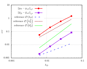
We evaluate the error decay considering a reference grid of approximatively two millions of elements. Following [21] the analytical solution exhibit a singularity at $(0.5,0.25)$ and $(0.5,0.75)$ , to focus our attention only on the dependence the regularity of the solution on the error order, we consider a family of Cartesian meshes. The error history is presented in Figure 5a, which shows a pressure error for the both the sides of the fault is close to $\mathcal{O}\left(h_{\mathcal{D}}^{2}\right)$ . Moreover the pressure error for the porous medium is close to $\mathcal{O}\left(h_{\mathcal{D}}^{\frac{3}{2}}\right)$ , confirming the dependence of the error order to the regularity of the exact solution. Figure 5b shows the error of a particular mesh, highlight the two peaks of error close to the singularities.

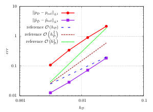
We consider also a different family of meshes for the error analyses, a coarser example is represented in Figure 3b. Each elements in the left part of the domain is constructed with 16 of small elements used for the right part. Even if the error is bigger then the previous case, both the pressure errors are close to $\mathcal{O}\left(h_{\mathcal{D}}^{\frac{3}{2}}\right)$ .

In Figure 6b we can see the different distribution of the error for the two sides of the domain, mainly present in its coarse part. Anyway, in each side, the error is concentrated close to the singularities.

4.2 Conductive fault

We consider the domain $\Omega=(0,1)^{2}$ with a vertical fault, of thickness $d=10^{-2}$ , in the centre of the domain, see Figure 7a for a sketch of the computational domain.

We assume homogeneous Neumann boundary conditions on the top and bottom of the domain, homogeneous Dirichlet boundary condition at left and Dirichlet boundary condition $p=1$ in the right part of the domain. We impose Dirichlet boundary conditions for both the ending of the fault, with value $p=1$ at the top and homogeneous at the bottom. Finally we consider identity matrix as permeability in the domain and in the fault we impose $\lambda_{f,\bm{{\tau}}}=10^{-2}$ and $\lambda_{f,\bm{{n}}}=1$ .

The computational mesh is composed by quadrangular elements, non-matching at the fault. The solution of (6) is depicted in Figure 8, we notice that the solution across the fault is continuous, as we expect, and the geometrical non-conformity is handled without any problem. The maximum and minimum discrete principle, in this particular experiment, are fulfilled.

To compute the error decay we consider a reference grid of approximatively two millions of elements. In Figure 9a we present the error history. The estimated order of the pressure error for the porous medium is a little lower then $\mathcal{O}\left(h_{\mathcal{D}}^{2}\right)$ . Moreover the error for the two layers of the fault is in between $\mathcal{O}\left(h_{\mathcal{D}}^{\frac{3}{2}}\right)$ and $\mathcal{O}\left(h_{\mathcal{D}}^{2}\right)$ , closer to the latter. If we suppose that the exact solution is continuous in $\Omega$ , then we have the numerical evidence of the second order of convergence of both the pressure in the porous medium and in the fault. In Figure 9b is represented an example of the error, we can notice that the highest error is close the both the ends of the fault, which is a normal behaviour.

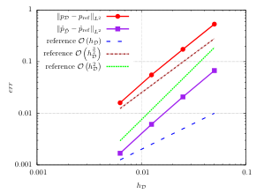
We consider also a different family of meshes for the error analyses, a coarser example is represented in Figure 3b. Each elements in the left part of the domain is constructed with 16 of small elements used for the right part. Also in this case both the pressure errors are close to $\mathcal{O}\left(h_{\mathcal{D}}^{2}\right)$ . Figure 10b shows the error for a particular mesh, also in this case it is concentrated close the two ends of the fault. As we expect the error is higher in the coarse part of the mesh.

We notice in both Figures 9b and 10b, especially in the right part of the domain for the latter, some oscillations in the error. Contrary to [21], in this case these spurious effects are due to a mesh effect. In Figure 11 we compute the error for a Cartesian mesh, the oscillations are not present.

4.3 Anisotropic fault

In this test case we present a much more involved example then the previous one, to verify the goodness of the numerical solution in presence of strong contrast in the mesh size. We consider the domain $\Omega=(0,1)^{2}$ with a vertical fault of width $d=10^{-2}$ . See Figure 12 for a sketch of the computational domain.

We impose homogeneous Neumann boundary conditions on the top and bottom of the domain and Dirichlet boundary conditions for the right and left part of the domain, as well as the fault. For the domain we assume $p=0$ on the left side and $p=1$ on the right side, while for the fault $p=0$ on the bottom and $p=1$ in the top. We consider identity matrix for the porous medium and, given $\lambda_{f}=100$ , for the fault

\displaystyle\Lambda_{f}(s)=\begin{bmatrix}\lambda_{f}&0\\ 0&\lambda_{f}^{-1}\end{bmatrix}\text{ for }s\in(0.25,0.75),\quad\Lambda_{f}(s)=\begin{bmatrix}\lambda_{f}^{-1}&0\\ 0&\lambda_{f}\end{bmatrix}\text{ for }s\in(0,0.25)\cup(0.75,1).

In its two extreme parts, the fault behaves as a low permeable strata for the flow across itself while as a channel for the flow inside. Vice versa for the other part of the fault, giving a solution with two singularities in the points $(0.5,0.25)$ and $(0.75,1)$ . We consider a family of meshes composed by fixed coarse discretization of the left part and a refined discretization of the right part of the domain.

In Figure 13 are reported different solutions for different meshes. The solutions keep in evidence the natural dependence on the mesh, which becomes much significant when the discretization of one side of the fault is much finer then the other side. In particular for Figure 13c the fine solution, in the central part of the fault, is almost flat in correspondence of each element of the coarse solution and exhibit a “jump” in correspondence of two different coarse elements. Anyway the obtained solution is reasonable.

$h_{\mathcal{D}}^{\rm max}/h_{\mathcal{D}}^{\rm min}$	1	2	4	8	16	32	64	128
AMG	8	10	10	11	11	12	12	12
ILU4	12	16	23	48	110	253	678	1462

Table 1: Number of iterations, for different mesh ratio

h_{\mathcal{D}}^{\rm max}/h_{\mathcal{D}}^{\rm min}

, to reach the convergence with to different preconditioners.

In Table 1 we present the number of iterations of a GMRES linear solver to obtain the solution of the problem. We consider a stopping criteria on the residual smaller then $10^{-12}$ , running the code only with one processor. In the table we consider two different preconditioner for the linear system: the algebraic multi-grid (AMG), form the Hypre library [19], and the incomplete LU factorization with level of fill equal to 4, from the library PETSc [8]. The result are quite promising for the AMG method since the number of iterations is almost constant, while for ILU4 the number of iterations increases at each refinement. Finally, even if an iteration of the ILU4 is cheaper in terms of CPU time than an iteration of the AMG, the numbers of iterations are so different that, from our experiments, we suggest to use the AMG method to solve also realistic problems.

4.4 Slipping domain

We consider now an example where one part of the domain slides, thanks to the fault, on the other part. The simulation is a sequence of problems in a moving domain: in its left side we have a deposition of sedimentary material and a movement from the top to the bottom of the sub-domain. The right part of the domain remains in the same position.

(a) Initial domain

t=t^{*}

(b) Final domain

t=T

Fig. 14: Representation of the meshes for two different configuration: the begin and the end of the simulation. The green cells are the discretization of

\Omega^{\rm barr}

In Figure 14 we present the domain at two different times: in the left at the beginning of the simulation and in the right at the end of the simulation. In the former case we have $\Omega=(0,10)\times(-3,0)Km^{2}$ and in the latter $\Omega\subset(0,10)\times(-3.35,0)Km^{2}$ . The others configurations of $\Omega$ moves from Figure 14a to Figure 14b linearly in time. The fault thickness is $d=50m$ . The mathematical model is the following: given $\partial\Omega^{\rm top}$ the top part of the boundary condition and $t^{*}$ and $T$ the initial and final times, find $p$ such that

\displaystyle\begin{aligned} &c\Phi\dfrac{\partial p}{\partial t}-\nabla\cdot\dfrac{\Lambda}{\mu}\nabla p=0&\quad&\text{in }\Omega\times(t^{*},T)\\ &\Lambda\nabla p\cdot\bm{{n}}=0&&\text{on }\partial\Omega\setminus\partial\Omega^{\rm top}\times(t^{*},T)\\ &p=0&&\text{on }\partial\Omega^{\rm top}\times(t^{*},T)\\ &p=p_{0}&&\text{in }\Omega\times\left\{t^{*}\right\}\end{aligned},

where $\mu=3.1\cdot 10^{4}Pa\cdot s$ is the dynamic viscosity. Considering Figure 14 we divide the domain $\Omega$ in the green part $\Omega^{\rm barr}$ , which behaves like a low permeable strata, and the remain part $\Omega\setminus\Omega^{\rm barr}$ . We impose as permeability and porosity and compressibility for the porous medium $\Lambda=\mathop{\operator@font diag}\nolimits\left(10^{-19}\right)m^{2}$ and $c\Phi=0.1\cdot 10^{-7}Pa^{-1}$ in $\Omega^{\rm barr}$ and $\Lambda=\mathop{\operator@font diag}\nolimits\left(10^{-15}\right)m^{2}$ and $c\Phi=0.5\cdot 10^{-7}Pa^{-1}$ in $\Omega\setminus\Omega^{\rm barr}$ . The initial and final times are: $t^{*}=-0.049My$ and $T=0.3My$ . The initial solution $p_{0}$ is computed, with domain in Figure 14a, thanks to the following problem

\displaystyle\begin{aligned} &-\nabla\cdot\dfrac{\Lambda}{\mu}\nabla p_{0}=0&\quad&\text{in }\Omega\\ &\Lambda\nabla p_{0}\cdot\bm{{n}}=0&&\text{on }\partial\Omega^{\rm left,right}\\ &p_{0}=0&&\text{on }\partial\Omega^{\rm top}\\ &p_{0}=10&&\text{on }\partial\Omega^{\rm bottom}\end{aligned},

with $\partial\Omega^{\rm left,right}$ is the left and right part of the $\partial\Omega$ and $\Omega^{\rm bottom}$ the bottom part of the domain. For the computation of $p_{0}$ we consider the permeability in the fault cells equal to the surrounding domain cell. The initial pressure is depicted in Figure 15.

We consider an implicit Euler scheme for the time discretization, no interpolation operator is considered in the left part of the domain. We consider now three different test to validate the model. In each test we change the value of the permeability inside the fault, while the porosity in the fault is equal to the porosity of the surrounding porous medium. In all the images we present both the pressure and the Darcy velocity, the latter using arrows with size $\chi$ -times its magnitude. We change the parameter $\chi$ to enhance the readability.

As a first test, represented in Figure 16 and 17, we present a sequence of solutions for different time steps. For each cell in each layer of the fault we consider the permeability equal to the permeability of the surrounding porous media. Then for certain time steps the three layers open one after the other leading to a pressure drop.

We notice that the Darcy velocity is very small before the opening of a low permeable strata, while increases after the opening. Then once one of this strata is opened, for example in Figure 17b, the flow starts to enter in the upper layers while the flow in the others layers tends to spread far from the centre of the domain. Moreover we have a pressure decrease, especially close to the fault, for each time step.

In Figure 18 we consider a second test case where the permeability in the fault is set to $\Lambda_{f}=\mathop{\operator@font diag}\nolimits\left(10^{-13}\right)m^{2}$ , so the fault behaves like a channel for the flow. To limit the evolution of the pressure we impose the porosity and compressibility as $c\Phi=10^{-6}Pa^{-1}$ in $\Omega^{\rm barr}$ and $c\Phi=0.2\cdot 10^{-6}Pa^{-1}$ elsewhere. Considering Figure 18a we see a pressure drop of the cells close to the fault, which is bigger in the bottom part of the domain where the pressure is higher. All the arrows of the Darcy velocity are almost parallel to the abscissa and pointing to the fault.

In the second and third images of Figure 18 we have the same phenomena but, since in the last time step the pressure is lower, the Darcy velocity is higher for $k=9$ than for $k=15$ . We see that for the pressure inside the green cells this behaviour is less evident.

The last test, depicted in Figure 19, represents an almost impermeable fault with permeability $\Lambda_{f}=\mathop{\operator@font diag}\nolimits\left(10^{-17}\right)m^{2}$ . The fault is more permeable than $\Omega^{\rm barr}$ but less permeable than $\Omega\setminus\Omega^{\rm barr}$ .

We have a very slow movement of the pressure during the simulation due to the nature of the fault. Since the permeability of the fault is in between the permeabilities of the porous media, once one layer of $\Omega^{\rm barr}$ is opened the fluid starts to flow up. Contrary to the first test case considered the end pressure is higher and the factor $\chi$ is six times higher bigger.

Remark 2 (Maximum principle).

We have tried to decrease the fault thickness until $d=10^{-1}m$ . In this case we have noticed that, for the last time step, the maximum principle is evidently violated. The maximum of the pressure, which is reached in the bottom cells, is a little bigger then $10MPa$ . Even if the value of the thickness is unphysical for our applications, this behaviour is a limitation of the proposed scheme. A possible explanation is the presence of the small cells with non-matching neighbours cells.

5 Conclusion

In this work we have derived and analysed a RM for single-phase flows in presence of faults, which can act as low permeable strata or channels. We consider faults that cut entirely the domain dividing the latter in disjoint parts. The proposed model allows to handle a domain in which one part can slip, along the fault past to the other. To easily handle the aforementioned properties we consider a mesh for each part of the domain independent from the meshes of other parts. The derivation of the mathematical model is similar to [30, 32], yet here we have used a different discretization scheme: the hybrid finite volume scheme [16], where one of the advantages is the presence of degrees of freedom on faces which help the approximation of the interface terms. Well posedness analyses has been given for the continuous problem as well as a convergence result for the discrete solution to the exact one. We have also shown several numerical experiments to estimate the convergence rates of the errors for both the porous medium and the fault. The examples highlight also the capability of the proposed method to handle different data configurations as well as the robustness with respect to the mesh size ratio between different parts of the domain.

6 Acknowledgements

The authors warmly thank Jérôme Jaffré and Jean E. Roberts for many fruitful discussions.

References

[1] Pierre M. Adler and Jean-François Thovert. Fractures and fracture networks. Springer, 1999.
[2] Pierre M. Adler, Jean-François Thovert, and Valeri V. Mourzenko. Fractured Porous Media. Oxford University Press, 2012.
[3] Clarisse Alboin, Jérôme Jaffré, Jean E. Roberts, and Christophe Serres. Modeling fractures as interfaces for flow and transport in porous media. In Fluid flow and transport in porous media: mathematical and numerical treatment (South Hadley, MA, 2001), volume 295 of Contemp. Math., pages 13–24. Amer. Math. Soc., Providence, RI, 2002.
[4] Clarisse Alboin, Jérôme Jaffré, Jean E. Roberts, Xuewen Wang, and Christophe Serres. Domain decomposition for some transmission problems in flow in porous media, volume 552 of Lecture Notes in Phys., pages 22–34. Springer, Berlin, 2000.
[5] Laila Amir, Michel Kern, Vincent Martin, and Jean E. Roberts. Décomposition de domaine et préconditionnement pour un modèle 3D en milieu poreux fracturé. In Proceeding of JANO 8, 8^th conference on Numerical Analysis and Optimization, December 2005. 2005.
[6] Philippe Angot. A model of fracture for elliptic problems with flux and solution jumps. Comptes Rendus Mathematique, 337(6):425–430, 2003.
[7] Philippe Angot, Franck Boyer, and Florence Hubert. Asymptotic and numerical modelling of flows in fractured porous media. M2AN Math. Model. Numer. Anal., 43(2):239–275, 2009.
[8] Satish Balay, Jed Brown, Kris Buschelman, Victor Eijkhout, William D. Gropp, Dinesh Kaushik, Matthew G. Knepley, Lois Curfman McInnes, Barry F. Smith, and Hong Zhang. PETSc users manual. Technical Report ANL-95/11 - Revision 3.4, Argonne National Laboratory, 2013.
[9] Jacob Bear, Chin-Fu Tsang, and G de Marsily. Flow and contaminant transport in fractured rock. Academic Press, San Diego, 1993.
[10] Brian Berkowitz. Characterizing flow and transport in fractured geological media: A review. Advances in Water Resources, 25(8-12):861–884, 2002.
[11] Franco Brezzi and Michel Fortin. Mixed and Hybrid Finite Element Methods, volume 15 of Computational Mathematics. Springer Verlag, Berlin, 1991.
[12] Carlo D’Angelo and Anna Scotti. A mixed finite element method for Darcy flow in fractured porous media with non-matching grids. Mathematical Modelling and Numerical Analysis, 46(02):465–489, 2012.
[13] Jérôme Droniou, Robert Eymard, Thierry Gallouët, and Raphaàele Herbin. A unified approach to mimetic finite difference, hybird finite volume and mixed finite volume methods. Mathematical Models and Methods in Applied Sciences, 20(02):265–295, 2010.
[14] Ahmed Elyes, Jaffré Jérôme, and Jean E. Roberts. A 3-D reduced fracture model for two-phase flow in porous media with a global pressure formulation. In MAMERN VI, Pau, France, June 2015.
[15] Alexandre Ern and Jean-Luc Guermond. Theory and Practice of Finite Elements. Applied mathematical sciences. Springer, 2004.
[16] Robert Eymard, Thierry Gallout, and Raphaèle Herbin. Discretization of heterogeneous and anisotropic diffusion problems on general nonconforming meshes sushi: a scheme using stabilization and hybrid interfaces. IMA Journal of Numerical Analysis, 30(4):1009–1043, 2010.
[17] Isabelle Faille, Eric Flauraud, Frédéric Nataf, Sylvie Pégaz-Fiornet, Frédéric Schneider, and Françoise Willien. A New Fault Model in Geological Basin Modelling. Application of Finite Volume Scheme and Domain Decomposition Methods. In Finite volumes for complex applications, III (Porquerolles, 2002), pages 529–536. Hermes Sci. Publ., Paris, 2002.
[18] Isabelle Faille, Alessio Fumagalli, Jérôme Jaffré, and Jean E. Roberts. Model reduction and discretization using hybrid finite volumes of flow in porous media containing faults. Computational Geosciences, 20(2):317–339, 2016.
[19] Robert D. Falgout and Ulrike Meier Yang. hypre: A library of high performance preconditioners. In PeterM.A. Sloot, AlfonsG. Hoekstra, C.J.Kenneth Tan, and JackJ. Dongarra, editors, Computational Science - ICCS 2002, volume 2331 of Lecture Notes in Computer Science, pages 632–641. Springer Berlin Heidelberg, 2002.
[20] Luca Formaggia, Alessio Fumagalli, Anna Scotti, and Paolo Ruffo. A reduced model for Darcy’s problem in networks of fractures. ESAIM: Mathematical Modelling and Numerical Analysis, 48:1089–1116, 7 2014.
[21] Najla Frih, Vincent Martin, Jean E. Roberts, and Ai Saâda. Modeling fractures as interfaces with nonmatching grids. Computational Geosciences, 16(4):1043–1060, 2012.
[22] Alessio Fumagalli and Anna Scotti. A numerical method for two-phase flow in fractured porous media with non-matching grids. Advances in Water Resources, 62, Part C(0):454–464, 2013. Computational Methods in Geologic CO2 Sequestration.
[23] Alessio Fumagalli and Anna Scotti. A Reduced Model for Flow and Transport in Fractured Porous Media with Non-matching Grids. In Andrea Cangiani, Ruslan L. Davidchack, Emmanuil Georgoulis, Alexander N. Gorban, Jeremy Levesley, and Michael V. Tretyakov, editors, Numerical Mathematics and Advanced Applications 2011, pages 499–507. Springer Berlin Heidelberg, 2013.
[24] Alessio Fumagalli and Anna Scotti. An Efficient XFEM Approximation of Darcy Flows in Arbitrarily Fractured Porous Media. Oil and Gas Sciences and Technologies - Revue d’IFP Energies Nouvelles, 69(4):555–564, April 2014.
[25] Bin Gong, Guan Qin, Craig Douglas, and Shiyi Yuan. Detailed Modeling of the Complex Fracture Network of Shale Gas Reservoirs. SPE Reservoir Evaluation & Engineering, 2011.
[26] Gilles Grospellier and Benoit Lelandais. The arcane development framework. In Proceedings of the 8th Workshop on Parallel/High-Performance Object-Oriented Scientific Computing, POOSC ’09, pages 4:1–4:11, New York, NY, USA, 2009. ACM.
[27] Jérôme Jaffré, Vincent Martin, and Jean E. Roberts. Generalized cell-centered finite volume methods for flow in porous media with faults. In Finite volumes for complex applications, III (Porquerolles, 2002), pages 343–350. Hermes Sci. Publ., Paris, 2002.
[28] Jérôme Jaffré, Mokhles Mnejja, and Jean E. Roberts. A discrete fracture model for two-phase flow with matrix-fracture interaction. Procedia Computer Science, 4:967–973, 2011.
[29] Mohammad Karimi-Fard, Louis J. Durlofsky, and Khalid Aziz. An Efficient Discrete-Fracture Model Applicable for General-Purpose Reservoir Simulators. SPE Journal, 9(2):227–236, 2004.
[30] Vincent Martin, Jérôme Jaffré, and Jean E. Roberts. Modeling Fractures and Barriers as Interfaces for Flow in Porous Media. SIAM J. Sci. Comput., 26(5):1667–1691, 2005.
[31] Alfio Quarteroni and Alberto Valli. Numerical Approximation of Partial Differential Equations, volume 23 of Springer Series in Computational Mathematics. Springer-Verlag, Berlin, 1994.
[32] Xavier Tunc, Isabelle Faille, Thierry Gallouët, Marie Christine Cacas, and Pascal Havé. A model for conductive faults with non-matching grids. Computational Geosciences, 16:277–296, 2012.

A double-layer reduced model for fault flow on slipping domains with hybrid finite volume scheme

Abstract

keywords

AMS

1 Introduction

2 Mathematical problem

2.1 Physical equations

Theorem 1.

2.2 The reduced model

Remark 1.

2.3 Weak formulation

Lemma 2 (Well posedness).

Proof.

3 Numerical approximation

Definition 3 (Discretization of Ω1,2\Omega_{1,2}).

Hypotheses 1 (Normal discrepancy).

Lemma 4 (Norm equivalence).

Proof.

Lemma 5 (Weak discrete 𝒱^\hat{{\mathcal{V}}} compactness).

Proof.

Lemma 6 (Discrete tangential gradient consistency).

Proof.

Lemma 7 (Convergence for matching grids).

Proof.

4 Examples

4.1 Partially impermeable fault

4.2 Conductive fault

4.3 Anisotropic fault

4.4 Slipping domain

Remark 2 (Maximum principle).

5 Conclusion

6 Acknowledgements

References

Definition 3 (Discretization of $\Omega_{1,2}$ ).

Lemma 5 (Weak discrete $\hat{{\mathcal{V}}}$ compactness).