Quantum knots in Bose–Einstein condensates created by counterdiabatic control

The mean-field order parameter of the spin-1 BEC can be written as $\Psi({\bf r},t)=\sqrt{n({\bf r},t)}e^{i\phi({\bf r},t)}\zeta({\bf r},t)$. Here, the $n$ is the particle density, $\phi$ is the scalar phase, and $\zeta=(\zeta_{+1},\zeta_{0},\zeta_{-1})^{T}_{\mathrm{Z}}$ is the complex-valued three-component spinor with $\zeta^{\dagger}\zeta=1$. The subscript in the spinor components refers to the magnetic quantum number of the $z$-quantized spin states $\left\{\left|+1\right>,\left|0\right>,\left|-1\right>\right\}$.

In the simulations, the condensate dynamics is solved within the mean-field approximation according to the Gross–Pitaevskii (GP) equation

where we employ the external optical potential $V({\bf r})=m\left[\omega_{\rho}^{2}\left(x^{2}+y^{2}\right)+\omega_{z}^{2}z^{2}\right]/2$ and the external magnetic field ${\bf B}({\bf r},t)$. The Cartesian vector ${\bf F}=(F_{x},F_{y},F_{z})$ is composed of the standard dimensionless spin-1 matrices. The coupling constants for the density and spin interactions are $c_{0}=4\pi\hbar^{2}(a_{0}+2a_{2})/(3m)$ and $c_{2}=4\pi\hbar^{2}(a_{2}-a_{0})/(3m)$ [41, 42], respectively, where the $s$-wave scattering lengths for ⁸⁷Rb are given by $a_{0}=5.387$ nm and $a_{2}=5.313$ nm [43], and the atomic mass by $m=1.443\times 10^{-25}$ kg. Furthermore, $g_{F}=-1/2$ is the Landé $g$ factor for ⁸⁷Rb, $\hbar$ is the reduced Planck’s constant, and $\mu_{\text{B}}$ is the Bohr magneton. The number of atoms is set to $N=2.1\times 10^{5}$, and the trapping frequencies to $\omega_{\rho}=2\pi\times 124~\mathrm{Hz}$ and $\omega_{z}=2\pi\times 248~\mathrm{Hz}$ throughout the simulations, corresponding to an oblate condensate.

The knot structures are created in the polar-phase order parameter of the spin-1 BEC using spatially and temporally varying external magnetic fields. For ⁸⁷Rb, the coupling constant $c_{2}$ is negative, implying ferromagnetic interactions in the absence of external magnetic fields. At low magnetic fields, the polar phase is dynamically unstable and decays into the ferromagnetic phase. However, the timescale for the decay due to this instability exceeds the knot creation time in the presence of magnetic field gradient [24, 9].

Taking the Euler angles $\alpha$, $\beta$, and $\gamma$ as successive rotations about $z$, $y$, and $z$ axes, respectively, the general spinor in the polar phase becomes [42]

where $\mathcal{U}=e^{-i\alpha F_{z}}e^{-i\beta F_{y}}e^{-i\gamma F_{z}}$. In the last identity we have expressed the spinor using the real-valued unit vector $\hat{\bf d}=(d_{x},d_{y},d_{z})^{T}=(\cos\alpha\sin\beta,\sin\alpha\sin\beta,\cos\beta)^{T}$, referred to as the nematic vector. It defines the direction of magnetic order in the condensate. Using this vector, we can express the order parameter in the Cartesian basis as $\Psi=\sqrt{n}e^{i\phi}\hat{\bf d}$.

The order parameter space for the polar spin-1 BEC is $\mathcal{O}_{\mathrm{P}}=\left[\mathrm{U}(1)\times S^{2}\right]/\mathbb{Z}_{2}$ [44], where the $\mathrm{U}(1)$ symmetry is attributed to the scalar phase $\phi$ and the $S^{2}$ symmetry to the vector $\hat{\bf d}$. Furthermore, the order parameter is invariant under the simultaneous transformations $\hat{\bf d}\rightarrow-\hat{\bf d}$ and $\phi\rightarrow\phi+\pi$, giving rise to the division by $\mathbb{Z}_{2}$ in $\mathcal{O}_{\mathrm{P}}$.

The nontriviality of the third homotopy group of the polar order parameter, $\pi_{3}(\mathcal{O}_{\mathrm{P}})\cong\mathbb{Z}$, allows the existence of knot structures in this phase. The related topological invariant, the Hopf charge $Q$, is defined as [3, 8]

where $\mathcal{F}_{ij}=\hat{\bf d}\cdot(\partial_{i}\hat{\bf d}\times\partial_{j}\hat{\bf d})$ and $\mathcal{A}_{i}$ is implicitly defined by $\mathcal{F}_{ij}=\partial_{i}\mathcal{A}_{j}-\partial_{j}\mathcal{A}_{i}$. We note that $\mathcal{A}_{i}$ can be defined up to a gauge $\mathcal{A}_{i}\rightarrow\mathcal{A}_{i}+\partial_{i}\eta$, where $\eta$ is a scalar function. For the sake of convenient integration in Eq. (3), one may choose such a gauge that one of the components of $\mathcal{A}$ is zero.

Previously, knots have been created in an initially nematicly $z$-polarized BEC by suddenly introducing a quadrupole magnetic field $b_{\mathrm{q}}(x\hat{\bf x}+y\hat{\bf y}-2z\hat{\bf z})$ in the middle of the condensate [8, 9]. Here, $b_{\mathrm{q}}$ is the strength of the gradient magnetic field. In the following discussion, we utilize the scaled coordinate system $(x^{\prime},y^{\prime},z^{\prime})=(x,y,2z)$ for convenience. The spin rotations leading to the knot configuration in Refs. [8, 9] are induced by the linearly increasing Larmor angular frequency $\omega_{\mathrm{L}}(r^{\prime})=g_{F}\mu_{\mathrm{B}}b_{\mathrm{q}}r^{\prime}/\hbar$, where $r^{\prime}=\sqrt{x^{\prime 2}+y^{\prime 2}+z^{\prime 2}}$. Knots with $Q=1$ are generated by allowing the Larmor precession to continue for $T_{\mathrm{L}}=2\pi\hbar/(g_{F}\mu_{\mathrm{B}}b_{\mathrm{q}}R^{\prime})$, where $R^{\prime}$ is the effective extent of the condensate. Thus the nematic vector experiences a full $2\pi$ rotation at radius $R^{\prime}$.

Here, in contrast, we show that the knot configuration can be created using a dynamic magnetic field control obtained from the CD scheme [39, 40]. In the CD scheme, we first select the reference adiabatic dynamics of the spin degree of freedom corresponding to the instantaneous eigenstates of the Zeeman Hamiltonian $\mathcal{H}_{\mathrm{Z}}=g_{F}\mu_{\mathrm{B}}{\bf B}({\bf r},t)\cdot{\bf F}$. In general, the CD magnetic field for a spin-1 system in the presence of a changing magnetic field ${\bf B}({\bf r},t)$ can be calculated with [38]

Our starting point is to design the CD field for the case in which the bias field is linearly inverted as ${\bf B}_{\mathrm{bias}}(t)=B_{0}(1-2t/T)\hat{\bf z}$, where $B_{0}$ is the initial bias field strength and $T$ is the inversion time while $b_{\mathrm{q}}$ is kept fixed. Hereafter, the time $T$ is referred to as the knot creation time. Furthermore, we employ the cylindrical coordinate system $(\rho,\varphi,z)$ below.

Application of the bias field inversion scheme directly into Eq. (4) leads to a CD field which rotates the nematic vector by $\pi$ everywhere. However, here we further set $z=0$ and $\rho=\rho_{0}$ [40]. The thus employed magnetic field coincides with the original CD field only on the ring with radius $\rho_{0}$ in the $z=0$ plane, along which the nematic vector undergoes a $\pi$-rotation during the inversion of the bias field (see Fig. 1). This ring is referred to as the core of the knot structure. Indeed, a knot with $Q=1$ corresponds to the parameter choice $\rho_{0}=R/2$, where $R$ is the effective extent of the condensate in the $z=0$ plane. Since the Larmor precession increases linearly as a function of distance from the origin, the nematic vector experiences a full $2\pi$ rotation at radius $2\rho_{0}=R$ so that the order parameter assumes a constant value at the condensate boundary. Along the $z$-axis the vector also retains its initial orientation. The nematic vector changes smoothly between these values. In practice, these rotations are induced by the brief pulse of magnetic field gradient near $t=T/2$, as is evident from the analytic form of the employed CD magnetic field shown below.

We further employ the unitary transformation introduced in Refs. [39, 40] to obtain a CD field which can be experimentally implemented using a single pair of quadrupole coils. The transformation is given by $U(t)=e^{-i\alpha(t)F_{z}}$, where $\alpha(t)=\arctan\left[|{\bf B}_{\mathrm{CD}}|/\left(b_{\mathrm{q}}\rho\right)\right]$. As a result, the Zeeman part of the Hamiltonian for the unitary-transformed order parameter is rotated by $\alpha(t)$ and an additional time-dependent magnetic field is introduced along $z$. The resulting magnetic field giving rise to the knot structure is [40]

where

and,

The control scheme of the magnetic field is presented in Fig. 2. In contrast to the control protocols used in Refs. [8, 9], the magnetic field zero point is not required to be centered in the middle of the condensate during the knot creation process, which is one of the most challenging experimental tasks [23]. At the end of our creation protocol, the magnetic field zero point is naturally located far away from the condensate, whereas in Refs. [8, 9] an additional control sequence is needed to achieve this condition. As we show below, by varying the parameter $\rho_{0}$ to a smaller value, our method allows for a convenient creation of knots with higher Hopf charge than that reported in Refs. [8, 9].

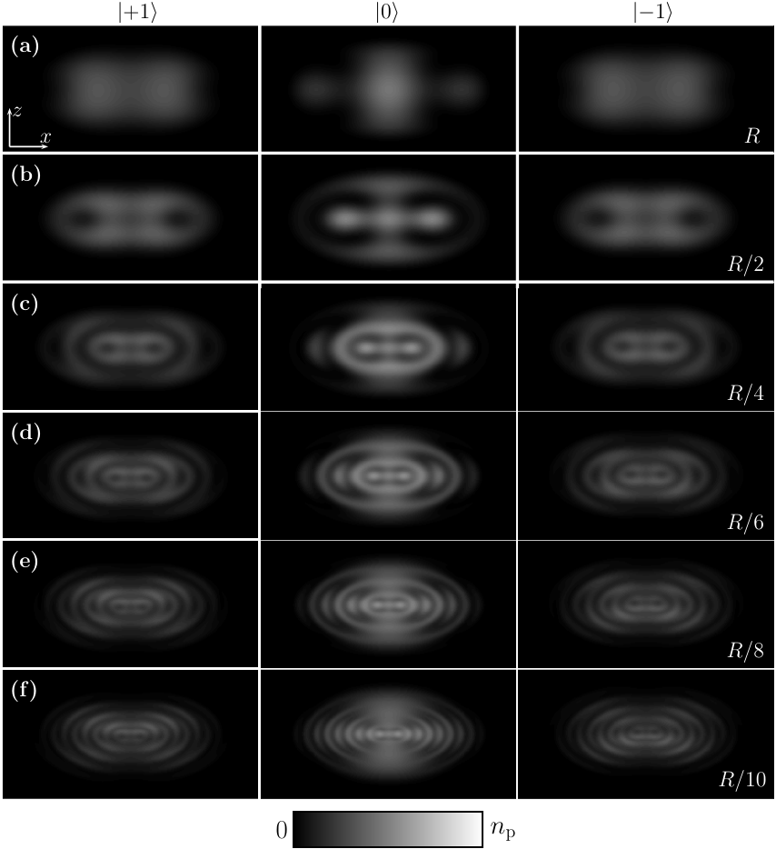
Figure 3 shows the $y$-integrated particle density distributions of different spinor components for various knot creation times. Here, we choose $\rho_{0}=R/2$ corresponding to a knot with the Hopf charge $Q=1$. For $T\leq 1.0~\mathrm{ms}$ we numerically confirm the Hopf charge to be unity. The componentwise densities are also consistent with the knot structure: $\zeta_{0}$ component, corresponding to $\hat{\bf d}$ pointing to positive or negative $z$ [see Eq. (2)], fills the central region and the boundary, as well as the core around the central axis of the condensate. The combination of $\zeta_{\pm 1}$ components, corresponding to $\hat{\bf d}$ residing along the $xy$-plane, fills the toroidal volume in between the $\zeta_{0}$ component [9].

Ideally, the spin density vanishes for the polar phase. However, the spin density increases with the knot creation time, indicating a transition from the polar state to the ferromagnetic state in the condensate. We attribute the destruction of the knot structure at long creation times to this transition. The rapid decay of the polar phase is due to the spatial variations in the nematic vector field leading to spin currents [8]. The transition to the ferromagnetic phase is further evidenced by the spatially separated $\zeta_{\pm 1}$ states for $T=2.0~\mathrm{ms}$.

The calculated preimages of $\hat{\bf d}=\hat{\bf x}$ and $\hat{\bf d}=-\hat{\bf x}$, shown in Fig. 4, display two linked rings. The preimages are closed curves in real space, along which the nematic vector points to a constant direction. The linked structure starts to depart from the conventional Hopf link as the knot creation time increases. Finally, for $T>1.0~\mathrm{ms}$, the link cannot be identified and the Hopf charge vanishes.

The particle densities and the calculated preimages for various choices of $\rho_{0}$ are shown in Figs. 5 and 6, respectively, with $T=0.1~\mathrm{ms}$ and $B_{0}=50~\mathrm{mG}$. The calculated Hopf charge increases with decreasing $\rho_{0}$ and the particle density distributions show the increase in the number of knot cores as $\rho_{0}$ decreases. The particle density distributions are consistent with those of multiple nested knot structures. The number of linked rings in the preimages increases according to the Hopf charge.

In the cases with Hopf charge $Q>1$, two linked rings appear $Q$ times in a nested structure, as is evident from the preimages in Fig. 6(c–f). These cases require a more careful topological inspection. Let us take $Q=2$ as an example and, for clarity, consider the scaled coordinate system $(x^{\prime},y^{\prime},z^{\prime})=(x,y,2z)$ in which the condensate is spherical. The preimages of $\hat{\bf d}=\pm\hat{\bf x}^{\prime}$ display two Hopf links. The two links are disconnected from each other, such that the inner link resides in the region $r^{\prime}<R^{\prime}/2$ and the outer link in $R^{\prime}/2<r^{\prime}<R^{\prime}$. This holds for all choices of two different vectors $\hat{\bf d}\neq\hat{\bf z}^{\prime}$.

The preimage of $\hat{\bf d}=\hat{\bf z}^{\prime}$ includes a line along the $z^{\prime}$-axis as well as two spheres with radii $R^{\prime}$ and $R^{\prime}/2$. The inner sphere with radius $R^{\prime}/2$ can be compactified into a point, since $\hat{\bf d}=\hat{\bf z}^{\prime}$ throughout the surface, thus compactifying the three-dimensional ball with $r^{\prime}\leq R^{\prime}/2$ into $S^{3}$. This compactification procedure defines the usual Hopf map in the region $r^{\prime}\leq R^{\prime}/2$.

Topologically, the outer region is now homeomorphic to a three-dimensional ball with $r^{\prime}\leq R^{\prime}$ as the sphere at $r^{\prime}=R^{\prime}/2$ is compactified into a point as described above. The outer sphere at $r^{\prime}=R^{\prime}$ is further compactified into another point, giving rise to another appearance of the Hopf map in the region $R^{\prime}/2\leq r^{\prime}\leq R^{\prime}$. Similar compactification procedures can be applied for the cases with $Q>2$, giving rise to the $Q$-fold nested Hopf maps.