Elastic amplitudes studied with the LHC measurements at 7 and 8 TeV
Abstract
Recent measurements of the differential cross sections in the forward region of pp elastic scattering at 7 and 8 TeV show precise form of the dependence. We propose a detailed analysis of these measurements including the structures of the real and imaginary parts of the scattering amplitude. A good description is achieved, confirming in all experiments the existence of a zero in the real part in the forward region close to the origin, in agreement with the prediction of a theorem by A. Martin, with important role in the observed form of . Universal value for the position of this zero and regularity in other features of the amplitudes are found, leading to quantitative predictions for the forward elastic scattering at 13 TeV.
I LHC experiments in elastic scattering
With an enormous gap in the center-of-mass energy with respect to previous data in pp and scattering, the Totem and Atlas experimental groups at LHC have recently measured in forward ranges at = 7 and 8 TeV [1, 2, 3, 4]. These measurements offer a unique opportunity to investigate the behaviour of p-p collisions at the highest energies reached in laboratory. A detailed and precise analysis of these data can establish a precious milestone for the understanding of the high energy behaviour of p-p interactions. The datasets and their ranges are listed in Table 1, where we use obvious notation T7, T8, A7, A8 to specify Totem (T) and Atlas (A) Collaborations and center-of-mass energies 7 and 8 TeV.
| dataset | range | N | Ref. | |||||
| (GeV) | points | (mb) | ( GeV | |||||
| 7 | Totem T7 | 0.005149-0.3709 | 87 | 1 | 98.62.2 | 19.90.3 | 0.14 (fix)a | |
| 7 | Atlas A7 | 0.0062-0.3636 | 40 | 2 | 0.14 (fix) b | |||
| 8 | Totem T8 | 0.000741-0.19478 | 60 | 3 | 19.56 0.13 | (0.12 0.03) c | ||
| 8 | Atlas A8 | 0.0105-0.3635 | 39 | 4 | 0.1362 (fix)d |
In order to build a bridge towards theoretical models aiming at the understanding of the dynamics, it is important that the analysis of these LHC data be made with identification of the structures of the individual parts of the complex scattering amplitude. The disentanglement of the two terms in the observed modulus is the crucial task. At each energy, parameterizations must search to exhibit clearly the properties of magnitudes, signs, slopes and zeros of the real and imaginary parts. External support, as dispersion relations and connections with analyses at other energies, give important clues. The intervention of the electromagnetic interactions must be treated coherently with a proposed analytical form for the nuclear part, and account must be taken of phase of the Coulomb-Nuclear Interference (CNI), which is calculated in Appendix A.
In the present work we perform a detailed examination of the data trying to satisfy these requirements. Each part of the amplitude is written with an exponential factor with a slope, multiplying a linear term in , thus with three parameters. These analytical forms are sufficient to describe the properties of the nuclear parts. The six parameters for each dataset are studied using fits to data with appropriate statistical control. Correlations are studied, and resulting values are proposed for each dataset. Good description of the measurements is obtained, with details in the shape of the forward diffractive peak, exhibiting the zero of the real part predicted in the theorem by A. Martin [5], and with observation in the forward range of the ingredients that construct the imaginary zero responsible for the dip in observed when data exist at higher .
According to analyses and models of pp and scattering at high energies [6, 7, 8], including full- ranges, the imaginary part has a zero near the marked dip observed in at about 0.4-0.6 , while the real part starts positive at , has a zero for small (Martin’s theorem), and a second zero after the dip. The descriptions of the models differ for higher about the position of this second real zero and about the existence of further imaginary or real zeros. Models describing large ranges have different motivations and dynamical structures, and may be analytically very sophisticated, trying to represent the observed shapes of dip, bump, tail, in the angular dependence. However in the forward range the analytical structure required to describe data may be very simple. In the present work we show that real and imaginary parts including exponential slopes and linear factors, combined with the electromagnetic interference, contain the essential ingredients for a precise representation. The second real zero occurs outside the studied range and does not influence the analysis. Particularly due to the small magnitude of the parameter, the disentanglement of the two parts is not trivial, requiring careful analysis, and still leaving room for some subjective but physically reasonable choice. Once the amplitudes are identified, the results provide a necessary connection between data and theoretical models of microscopic nature for the strong interaction dynamics.
The deviation from the pure exponential form in is obvious beforehand, since is a sum of two independent squares. More clarity can be obtained in the analysis with the identification of the two parts of the complex amplitude and their control by fundamental constraints (dispersion relations, Martin’s theorem for the real part, zero of the imaginary part anticipating the dip).
Of the four datasets, T8 is the only one reaching very small , allowing the more complete investigation of some details, such as the influence of the Coulomb phase. However a comparative analysis of the four cases is extremely important, since observing coherence in some characteristics we may believe that there is reliability in the descriptions. The energy dependence of pp elastic scattering is very smooth, and features of 7 and 8 TeV data must support each other in a unified treatment.
A theorem by André Martin proves that the real part has a zero close to the origin [5]. The abstract of the paper says, literally
We show that if for fixed negative (physical) square of the momentum transfer , the differential cross section tends to zero and if the total cross section tends to infinity, when the energy goes to infinity, the real part of the even signature amplitude cannot have a constant sign near . @ 1997 Elsevier Science B. V.
Thus the real part in pp and pp̄ scattering has a zero close to the origin, with location approaching as the energy increases. This constraint has been confirmed in previous analyses at LHC and lower energies [6, 7], with the conclusion that the position of the first zero of the real part behaves like
Although the analytical properties of the amplitude are defined in t-space, the insights for the construction of theoretical models are natural in the geometrical space, where the physical intuition to build amplitudes may be represented. The Fourier transformed space is appropriate to study asymptotic properties of the cross sections such as questioning whether the proton behaves as a black or a gray disk. The profile functions are also convenient tools to study the unitarity constraint. Of course we recognize that the amplitudes written for the short forward -range cannot lead to a sufficient understanding of -space properties. Even thus, we believe that the relationship is important, and the Fourier transformation of our amplitudes to -space is analytically performed and its properties discussed in Appendix B.
This paper is organized as follows. Section II describes the formalism of the proposed model; Section III presents the results of the model fits to the four LHC measurements; Section IV summarizes the numerical analysis ; Section V concludes the paper.
II Amplitudes and Observables in Forward Scattering
In the analysis limited to the forward ranges shown in Table 1, the expectations are satisfied writing the differential cross section in the form
| (1) |
where , is the fine structure constant and mb . This expression is applied for pp an pp̄, and the parameters are specific for each case. and represent the form factor and phase of the Coulomb interaction. The phase has opposite signs for pp and pp̄ sccattering.
The real electromagnetic amplitude is given in terms of the proton form factor
| (2) |
for the ppp collisions. The proton form factor is taken as
| (3) |
where . The phase of the Coulomb-Nuclear interference is discussed in Appendix A.
We have thus assumed the imaginary amplitude with an exponential that accounts for the forward diffractive peak and a linear factor that accounts for the zero that occurs near the dip in , writing the simple form
| (4) |
and
| (5) |
The influence of the parameter depends on the range of the data analyzed. To include the influence of the first real zero, we write
| (6) |
and
| (7) |
In order to check the influence of a second zero in the real part, we could add in the amplitude a term , but actually it has no effect in the present analysis.
The normalization is defined by
| (8) |
and for the pure nuclear interaction
| (9) |
At , we have the usual definition of the parameter
| (10) |
With positive and negative (this is what we have in pp at high energies, as our analysis shows), there is a zero in the real amplitude, namely Martin’s zero, located at
| (11) |
The position of this zero and the magnitudes of the real and imaginary amplitudes in its neighborhood are responsible for details in the deviation of the differential cross section from a pure exponential behaviour.
The derivatives of the nuclear amplitudes at are
| (12) |
and
| (13) |
The average slope measured directly in is the quantity
| (14) |
We remark that parameters are determined fitting data in limited ranges, at finite distance from the origin, so that the values obtained depend on the analytical forms (4,5,6,7) of the amplitudes. In particular, the slope parameter usually written in form does not agree with the expression for the differential cross section as sum of two independent squared magnitudes, each with its own slope. The assumption that and are equal is not justified. The average quantity alone gives rough and unsatisfactory information. The importance of the different slopes in the analysis of pp elastic scattering has been investigated in the framework of the so called dispersion relations for slopes [9]. It is important to note that also the Coulomb-Nuclear phase depends essentially on the form of the nuclear amplitudes [12]. In the Appendix A, generalizing previous work [13, 14, 6], we derive the expression for the phase to be used with the assumed amplitudes written above.
Of course the six parameters are correlated, and in the present work we investigate the bounds of the correlations. We attempt to identify values of parameters that may be considered as common representatives for different measurements. We show that the differences between the two experimental collaborations may be restricted to quantities characterizing normalization. The question of normalization is essential, and our inputs are the values of given in the experimental papers [1, 2, 3, 4].
The extraction of forward parameters in pp scattering has difficulties due to the small value of the parameter, and consequently has suffered in many analyses from neglect of the properties of the real part. In our view the values of , , appearing in universal databases [10, 11] as if they were direct experimental measurements should give room for critically controlled phenomenological determinations. A proper consideration for the properties of the complex amplitude is necessary. We observe that the properties that and of the presence of zeros are common to several models [6, 7, 8]. The determination of the amplitudes for all in several models is coherent.
We observe that the polynomial factors written in the exponent in some parameterizations of data [3] correspond to the linear and quadratic factors mentioned above, if the assumption is made that they are much smaller than 1 and can be converted into exponentials. However this substitution is not convenient, because it does not show explicitly the essential zeros, and it also gives unsatisfactory parameterization that cannot be extended even to nearby values.
We thus have the framework necessary for the analysis of the data, with clear identification of the role of the free parameters. The quantities to be determined for each dataset are , , , , , .
III Data analysis
| N | ndf | ||||||||||
| (mb) | |||||||||||
| Condition I) - all six parameters free | |||||||||||
| T8 | 60 | ff | 102.700.07 | 0.090.01 | 19.960.05 | 23.550.39 | -2.780.12 | -0.0010.023 | -0.0320.004 | 19.960.07 | 58.53/54 |
| T8 | 60 | 0 | 102.600.09 | 0.110.01 | 19.770.05 | 23.810.46 | -2.780.14 | -0.0490.023 | -0.0400.004 | 19.870.07 | 58.89/54 |
| A8 | 39 | ff | 97.020.52 | 0.110.08 | 16.500.94 | 22.761.22 | -3.370.24 | -1.650.41 | -0.0340.024 | 19.801.25 | 27.62/33 |
| A8 | 39 | 0 | 96.910.60 | 0.130.08 | 16.420.94 | 22.711.26 | -3.330.24 | -1.650.41 | -0.0370.024 | 19.721.24 | 27.51/33 |
| T7 | 87 | ff | 99.970.36 | 0.110.06 | 15.250.75 | 23.640.61 | -4.530.37 | -2.450.20 | -0.0240.013 | 20.150.85 | 93.48/81 |
| T7 | 87 | 0 | 99.820.43 | 0.130.06 | 15.100.72 | 23.480.60 | -4.450.36 | -2.460.19 | -0.0290.014 | 20.020.81 | 93.52/81 |
| A7 | 40 | ff | 95.770.16 | 0.000.04 | 15.551.06 | 21.740.49 | -4.030.65 | -2.360.58 | 0.0000.010 | 20.271.57 | 20.93/34 |
| A7 | 40 | 0 | 95.700.16 | 0.000.13 | 15.581.18 | 21.660.54 | -3.920.69 | -2.310.64 | 0.0000.033 | 20.201.74 | 20.58/34 |
| Condition II) - fixed (suggested by dispersion relations) | |||||||||||
| T8 | 60 | ff | 102.600.16 | 0.14 (fix) | 19.850.14 | 24.770.57 | -3.070.26 | -0.0030.274 | -0.0460.004 | 19.860.56 | 66.35/55 |
| T8 | 60 | 0 | 102.500.16 | 0.14 (fix) | 19.770.57 | 24.550.59 | -2.930.26 | -0.020.86 | -0.0480.004 | 19.811.81 | 61.29/55 |
| A8 | 39 | ff | 96.830.13 | 0.14 (fix) | 16.400.95 | 22.831.40 | -3.330.22 | -1.630.43 | -0.0420.003 | 19.661.28 | 27.71/34 |
| A8 | 39 | 0 | 96.800.13 | 0.14 (fix) | 16.360.92 | 22.741.35 | -3.310.22 | -1.640.42 | -0.0420.003 | 19.641.25 | 27.54/34 |
| T7 | 87 | ff | 99.830.20 | 0.14 (fix) | 16.110.13 | 25.001.77 | -4.210.33 | -1.970.10 | -0.0330.003 | 20.050.24 | 95.02/82 |
| T7 | 87 | 0 | 99.750.20 | 0.14 (fix) | 16.100.13 | 25.001.88 | -4.130.33 | -1.950.09 | -0.0340.003 | 20.000.22 | 94.94/82 |
| A7 | 40 | ff | 95.800.17 | 0.14 (fix) | 14.150.47 | 21.450.34 | -4.540.39 | -2.670.24 | -0.0310.003 | 19.490.67 | 25.95/35 |
| A7 | 40 | 0 | 95.730.17 | 0.14 (fix) | 14.150.49 | 21.370.35 | -4.470.39 | -2.650.25 | -0.0310.003 | 19.450.70 | 25.11/35 |
| Condition III) - [7] or [6] | |||||||||||
| T8 | 60 | ff | 102.600.14 | 0.080.02 | 15.500.11 | 20.790.44 | -3.470.19 | -2.16 (fix) | -0.0230.006 | 19.820.11 | 58.98/55 |
| T8 | 60 | 0 | 102.500.16 | 0.110.02 | 15.360.11 | 20.760.43 | -3.490.18 | -2.16 (fix) | -0.0320.006 | 19.680.11 | 59.55/55 |
| A8 | 39 | ff | 96.880.62 | 0.130.07 | 15.300.47 | 21.680.36 | -3.690.13 | -2.16 (fix) | -0.0360.019 | 19.620.47 | 29.96/34 |
| A8 | 39 | 0 | 96.750.69 | 0.140.07 | 15.220.46 | 21.600.35 | -3.660.12 | -2.16 (fix) | -0.0390.018 | 19.549.46 | 29.84/34 |
| T7 | 87 | ff | 100.000.23 | 0.080.09 | 16.070.43 | 24.380.49 | -4.350.37 | -2.14 (fix) | -0.0180.021 | 20.350.43 | 92.51/82 |
| T7 | 87 | 0 | 99.940.25 | 0.090.05 | 15.950.41 | 24.260.50 | -4.250.36 | -2.14 (fix) | -0.0210.012 | 20.230.41 | 94.38/82 |
| A7 | 40 | ff | 95.760.16 | 0.000.04 | 15.940.17 | 21.860.50 | -3.840.29 | -2.14 (fix) | 0.0000.010 | 20.220.17 | 21.01/35 |
| A7 | 40 | 0 | 95.690.16 | 0.000.12 | 15.890.17 | 21.760.51 | -3.780.29 | -2.14 (fix) | 0.0000.032 | 19.460.17 | 20.62/35 |
| Condition IV) - and [7] or [6] fixed as in II) and III) | |||||||||||
| T8 | 60 | ff | 102.400.15 | 0.14 (fix) | 15.270.39 | 21.150.39 | -3.690.15 | -2.16 (fix) | -0.0380.002 | 19.590.39 | 69.2/56 |
| T8 | 60 | 0 | 102.300.14 | 0.14 (fix) | 15.230.07 | 20.970.40 | -3.610.15 | -2.16 (fix) | -0.0390.002 | 19.550.07 | 63.14/56 |
| A8 | 39 | ff | 96.820.11 | 0.14 (fix) | 15.260.06 | 21.650.24 | -3.690.12 | -2.16 (fix) | -0.0380.001 | 20.030.14 | 29.97/35 |
| A8 | 39 | 0 | 96.780.11 | 0.14 (fix) | 15.240.06 | 21.610.23 | -3.660.12 | -2.16 (fix) | -0.0380.001 | 19.990.14 | 29.84/35 |
| T7 | 87 | ff | 99.800.21 | 0.14 (fix) | 15.710.14 | 24.260.47 | -4.240.31 | -2.14 (fix) | -0.0330.002 | 19.990.14 | 95.08/83 |
| T7 | 87 | 0 | 99.720.21 | 0.14 (fix) | 15.670.14 | 24.150.48 | -4.160.31 | -2.14 (fix) | -0.0340.003 | 19.950.14 | 94.98/83 |
| A7 | 40 | ff | 95.750.16 | 0.14 (fix) | 15.230.11 | 21.860.44 | -3.990.22 | -2.14 (fix) | -0.0350.002 | 19.510.11 | 27.33/36 |
| A7 | 40 | 0 | 95.680.16 | 0.14 (fix) | 15.190.11 | 21.770.44 | -3.940.22 | -2.14 (fix) | -0.0360.002 | 19.470.11 | 26.34/36 |
The range of covered in this analysis corresponds to a forward region, with from GeV2 for T8 to GeV2 for T7. In this range the Coulomb effects play important role and the relative Coulomb phase is taken into account. We compare results for the the relative phase , calculated in Appendix A with proton form factor () and the reference case of phase zero . This alternative is examined to set reference values because of possible lack of understanding of electromagnetic effects, as in the calculation of the phase and the possible influence of the proton radius at high energies.
The statistical methods used in analyzes are performed with CERN-ROOT software [17], accounting for statistical and systematics uncertainties. However, since the values of do not change much compared with the statistical uncertainties only, we understand that the statistical errors are enough for the analyses with our amplitudes.
We also study the correlation between the parameters, which is an useful tool to control possible instabilities of the fits. The correlations between the parameters are defined as
| (15) |
where and are any two parameters, the brakets are the expectation values of the fitted parameters and and the variances associated with them. This correlation criterion is known as Pearson coefficient and varies from -1 to 1, where -1 is a complete anti-correlation, meaning that if one parameter is increased the other one decreases, and 1 is a complete correlation which means that if one parameter is increased the other one also increases. If the correlation coefficient is zero the parameters are said non-correlated, or independent. The correlation factors help us to understand the relation between the determination of the parameter and the range of where this determination is performed.
With the purpose of identifying generic or universal values for parameters, for all measurements we study four different conditions in the fit:
- •
I) all six parameters are free ;
- •
II) fixing at 0.14, as suggested by dispersion relations;
- •
- •
IV) fixing simultaneously and at the above values.
We present our analysis for the four experiments separately in the next subsections. Since T8 has more precise data in the very forward region and the experimental paper has provided a detailed description of the observed structure, we investigate it with more detail. For this purpose we introduce a new diagram to represent the structure in the data at low , plotting the ratio against , with
| (16) |
This ratio does not depend on the total cross section, and therefore normalization uncertainties are cancelled, allowing identification of the zero in the real amplitude.
The results of the analysis are presented in Table 2. The headings of the table indicate the quantities determined in fits, namely the six parameters ,,,, and . Other columns give the derived quantities and , and the estimated values. The first three columns specify the measurement, with the number N of data points, and the phase option (either the true phase or the reference option of zero phase).
III.1 T8


The T8 dataset contains measurements with two different optics. The first set of data (30 points) covers a very forward region, , and the second set (30 points) starts a bit latter, , overlapping partially with the first, but with better statistical precision. They analyzed separately the first set, here called SET I, with 30 points, and the combination of the first and the second measurements, with N=60 points, here called SET II. Analyzing SET I they obtained . In the analysis with SET II, was not independently determined, but it was rather fixed at the same value of SET I.
Repeating this analysis in two steps, using our nuclear amplitudes and testing phase values and , we find that the determination of the parameter is critical, strongly influenced by points in the most forward region. Using Condition I), with all six parameters free, the results are the following. With SET I we obtain for case, which is a little bit bellow the expectation 0.14 from dispersion relations With the zero reference phase we obtain . With the complete SET II the values come out considerably smaller than in SET-I for both and phases, deviating still more strongly from 0.14. These results show the difficulty of T8 for free independent determination of the parameter .
SET II is used in the description that follows, and the resulting parameters are registered in Table 2.
Using the condition I) we obtain equivalent GeV-2 for both and phases, but since the values of are different the position of the zero changes from -0.032 0.004 GeV2 to -0.040 0.004 GeV2 for the and phases respectively. We remark that precise data in the vicinity of the zero is important for the determination of .
In Fig.1 we present the fit results of the T8 data with all parameters free, as in Condition I, and phase . The parametrization is able to describe the T8 measurements. With plots showing local displacements, shown in Fig. 2, we are able to exhibit details of the structure of the amplitudes. In the LHS we plot diagram similar to that presented in the paper of the experimental group [3], showing the valley structure appearing when we subtract the simple exponential form
from the best fit solution for the differential cross section. The structure appears neatly, but the band of normalization errors is very large, and the roles played by the amplitudes are not clear. In the right hand side of Fig. 2 the quantity shows the turning point due to the zero of the real part of the amplitude, with a much narrower band of the systematic errors due to the cancellation of dependence in the ratio.
The interplay of the magnitudes of the real and imaginary amplitudes influences the structure of . The deviation of a pure exponential behaviour is inherent to the sum of two independent squared quantities.
From the fits performed in T8 we obtain from the correlation coefficients that is weakly correlated with all other parameters. This is the reason why when we fix its value according to Conditions II) and IV) we obtain larger than with Condition I): other parameters are not able to compensate the change in .
In both conditions I) and II) the parameter of the imaginary part is very small, which means that the t-range in the data is not far enough to feel the zero of the imaginary amplitude. On the other hand, fixing in Condition III), is seen as strongly dependent on the phase.
It is important that, although the parameter has weak Pearson coefficients, the statistical error associated with this parameter is large, which means that it cannot be well determined with Condition I) or II). The values do not change considerably from Condition I) to Condition III), but the parameters , and change. The presence of non-zero negative obliges the imaginary amplitude to point towards zero. The real amplitude must compensate the decrease of the imaginary part, reducing the magnitude of the real slope, and the value of is also affected. The imaginary slope compensates the increase in the magnitude of introduced in III), thus preserving the value of .
Fig. 3 shows the correlation maps between pairs of parameters. These figures correspond to Pearson coefficients , and showing weak correlations for the first two cases, and a strong anti-correlation for the latter. The lines represent the allowed regions at different standard deviations. Since is weakly correlated with the parameters of the real part according to Condition III), in Condition IV) we expect small deviation in and . In this Condition we obtain very similar results for the free parameters for both choices of phase.
III.2 A8
In A8 [4] the Atlas Collaboration measured 39 points in the region . With Condition I) we obtain central values compatible with dispersion relations (namely 0.14), but with large error bars of 70. Showing insensitivity, the values of are similar for and phases. Although the values in A8 and T8 are different by 20%, the positions of the real zero differs about 6%. The real amplitudes for T8 and A8 are shown in Fig. 4 and we can clearly note that the position of the Martin’s zero is in agreement between the measurements.

Important differences between T8 and A8 are in the parameters of the imaginary part. Thus for A8, while for T8 it is compatible with zero due to the short range of the data.
The values of in A8 and T8 differ by . This difference may be due relative normalization, and we may ask whether a unification of through a constant factor could unify the solutions for , while leading also and to common values.
Since the fits for A8 show strong anti-correlation factor between and , and is a stable parameter, we use Condition II) to fix at 0.14 and obtain very similar to the result obtained in Condition I) with free , which is natural since in I), in not very different from 0.14. Under Condition II), with fixed , the results for T8 and A8 give compatible values.
In A8, for both I) and II), the parameter predicts which is far on the right of the region where the dip in is expected to occur. By fixing in Condition III), for A8 agrees with the value found in T8, as expected, since values of are in agreement for all Conditions.
The use of Condition IV) does not change considerably the parameters of A8 when compared with Condition III), because the central values of in III) are close to 0.14 .
III.3 T7
At =7 TeV the Totem Collaboration measured elastic p-p cross sections with two sets [1], the first in the range ( GeV2 ) with 87 points, and the second in the range GeV2 with 78 points. Using our expressions for the forward amplitudes, we analyze the forward set, obtaining the results shown in Table 2. With all parameters free, for both and phases the values are less than 0.14. The values for are similar to those in A8. The total cross section is higher but compatible with the original paper [1], as given in Table 1.
The correlation factor obtained in Condition I), shows a strong anti-correlation. Since is a stable parameter and the central value is larger than the expected 0.14, Condition II) fixing , leads for all other parameters and for results similar to Condition I).
With Condition III) we observe that the central values are smaller than obtained with I), and the statistical errors are about 55 () and 88 () of the central value.
Analysis of an Extended Set
| N | ndf | ||||||||||
| (mb) | |||||||||||
| Condition I) - all six parameters free | |||||||||||
| T7 | 87+17 | ff | 99.330.49 | 0.160.05 | 15.360.24 | 22.630.38 | -3.540.22 | -2.150.02 | -0.0450.014 | 19.660.24 | 203.1/98 |
| T7 | 87+17 | 0 | 99.180.52 | 0.170.05 | 15.300.24 | 22.510.39 | -3.470.21 | -2.140.02 | -0.0480.014 | 19.580.24 | 202.1/98 |
| Condition II) - fixed by dispersion relations | |||||||||||
| T7 | 87+17 | ff | 99.490.18 | 0.14 (fix) | 15.460.08 | 22.730.30 | -3.570.22 | -2.150.02 | -0.0390.002 | 19.760.09 | 203.3/99 |
| T7 | 87+17 | 0 | 99.420.17 | 0.14 (fix) | 15.430.08 | 22.650.30 | -3.520.22 | -2.150.01 | -0.0400.002 | 19.730.08 | 202.4/99 |
| Condition IV) - Fixed values and [6] | |||||||||||
| T7 | 87+17 | ff | 99.440.14 | 0.14 (fix) | 15.440.07 | 22.620.19 | -3.490.13 | -2.14 (fix) | -0.0400.002 | 19.720.07 | 203.5/100 |
| T7 | 87+17 | 0 | 99.390.14 | 0.14 (fix) | 15.430.07 | 22.590.19 | -3.470.13 | -2.14 (fix) | -0.0400.002 | 19.710.07 | 202.5/100 |
The special availability in T7 of data beyond the limit of the measurements in Table 1, may be used to study a range where the parameter becomes more effective, pointing towards the zero of the imaginary amplitude, and being determined with higher accuracy. We thus add to the forward set the first 17 points of the second dataset, reaching . The results of the analysis with the combined set of 104 points are presented in Table 3.
The study of the extended set with Condition I) leads to the correlation map for the quantities and shown in Fig. 5. The Pearson coefficient depends on the range on where the fit is made and of course the fit conditions used, and for this extended range it shows a slight anti-correlation between and .
In Fig. 6 we compare the squared magnitudes of the real and imaginary amplitudes, and also the simplified single exponential amplitude assuming the effective slope , for the extended T7 with Condition I). We observe that the imaginary part starts to deviate from the simple exponential near GeV2, and at GeV2 it passes through a zero. Beyond this range the real amplitude would be modified to incorporate other terms (say a quadratic ) that may play important role in the construction of the dip structure.
As with the forward set, here the values come out larger than 0.14, but within error bars. Fixing in Condition II), the changes in parameters and in are very small.
It is very important that the parameter is here determined with more precision and is compatible with the value fixed to establish Condition III) in Table 2.
The use of condition IV) for this extended set, shown in Table 3, leads to a decrease in the magnitudes of and when we compare with the results of the forward set under the same condition. Since is fixed, the decrease in implies in an increase in the magnitude of .


III.4 A7
In A7 the Atlas Collaboration measured [2] 40 points in the region . This experiment is challenging, since the experimental authors recognize that cannot be determined from the data with usual forms of amplitudes. The natural result for as a free parameter is a negative quantity, and we run Condition I) imposing a lower bound 0 for , and of course the expected value is zero, with large error bars. In this Condition the total cross section for phase is mb, which is well bellow, while the parameters , , and are compatible with T7. In these measurements the correlation factors between and all other parameters are very small. Thus with Condition II) we expect an obvious increase of , but the parameters , and are compatible with T7.
With Condition I), is compatible with zero, with large error. With Condition III), is not much changed, as well as the total cross section. The value is still undetermined but , and are compatible with the other experiments. Thus, in spite of the smaller value of total cross section and instabilities in the determination of , Condition IV) shows similar dependence in A7 with respect to the other datasets, with similar behaviour of the amplitudes.
IV Summary of the Analysis
The LHC measurements at = 7 and 8 TeV shown in Table I are analyzed under the assumption of the analytical forms for the scattering amplitudes given in Eqs. in Eqs. (4) and (6). These forms are considered as simple as possible under theoretical conditions to describe the scattering amplitudes in the forward region. The analysis aims at the determination of six intervening parameters, three for the imaginary part (,,) and three (, , ) for the real part, with expected smooth energy dependence. Only the T8 measurements cover very small range, so that the analysis is made with non-homogeneous inputs, and four specific Conditions, named I), II), III), IV) in Table 2, are studied separately.
The Coulomb-Nuclear interference is a crucial ingredient, and its phase is treated compatibly with the forms of the amplitudes, as presented in Appendix A. In order to have a reference (although not realistic) we also give results of fits with phase put equal to zero.
As expected, the direct results of the fits with all parameters kept free are rather dispersive in some aspects, as shown in the sub-table with title Condition I). The fitted values of do not agree among the measurements within the statistical uncertainties, but once the normalization uncertainty is considered, the values are in agreement. We observe that the other parameters of the real part ( and ), related to the shape of the amplitudes but not so strongly to its normalization, appear more regular.
In Condition II) is fixed at a reference value 0.14 suggested by dispersion relations for the 7-8 TeV range. Compared to I) there is a loss in in the cases with free far from 0.14, namely T8 and A7, but not in the other cases, where we observe only rather slight adaptation in the other real parameters: and appear as regular quantities. Also remains the same (except in A7), and it is particularly important to remark that the effective slope in Eq. (12), that compensates for the influence of on the dependence of the imaginary part, appears as a very regular common quantity. In spite of the differences, this point we may say that we are lead accept the value for all measurements. On the other hand, remains not regular among the experiments in this Condition II). Since is responsible for the presence of a zero () in the imaginary amplitude (that occurs near the dip in at about 0.4 ), it is natural that T8 (limited to 0.2 ) is not sensitive to , and puts it at zero in Conditions I) and II).
It is interesting to observe the effects of correlations. For instance, in T8 and A7 , is weakly correlated with the other parameters. Then, fixing in Condition II) worsens strongly for these datasets, more than in sets A8 and T7 where the strong correlation between and the other parameters absorbs the effects of the fixing condition. For T8 in case the worsening in is more dramatic, corroborating our concern about proton form-factor and Coulomb phase.
With Condition III) we fix according with the expected positions of the imaginary zero and dip in [7, 6], and let free. This is successful, as results about the same or improved with respect to Condition I) (all parameters free), except for A7, as expected. The parameters and of the real part remain the same, and it is remarkable that changes, becoming very regular, absorbing the influence of (now fixed) and keeping the constant and regular effective dependence of the imaginary amplitude, represented by .
The parameter determines a zero at in the imaginary amplitude and is related with the position of the dip in the differential cross section. A precise determination of depends on the existence of data in a region near the dip. Thus in the T8 dataset, without points for small , the central values of are near zero in I) and II), while in A8, T7 and A7 the values have larger magnitudes. We study this question analyzing the T7 experiment with inclusion of a second set of points [1]. Forming a larger dataset in the range , the best solution with fixed gives shown in Table 3, in good agreement with the prediction [7]. We are thus lead to Conditions III) and IV) that fix .
Fixing both and at their expected values in Condition IV) we obtain good modeling for all measurements, except for the total cross sections, that separate Atlas from Totem. It is particularly meaningful that the position of the zero of the real amplitude is nearly the same for all cases.
The deviation from pure exponential form in the differential cross section is interpreted as due to the shape difference between the real and imaginary amplitudes. The T8 experiment presents very precise data at low , showing a valley behaviour in the differential cross section, while the T7, A7 and A8 data also indicate a structure for the data at low , but with large uncertainties. The shape is constructed when the real amplitude crosses zero, passing to negative values. After the zero, the action of the real slope pushes this negative value back to zero, and the structure is formed.
This mechanism suggests that the determination of depends not only on the extrapolation to the limit at , but also depends on the form of the real amplitude around its zero. A precise extraction of depends both on the specific analytical model used and on the data in the whole range GeV2 where the valley occurs. The position of the real zero is obtained from the equation (values are given in Table 2).
Important quantities are the derivatives of the amplitudes and their effective slopes determined in each measurement. The exponent written in Eq. (4) is not the logarithmic derivative of the imaginary amplitude, that is given by Eq.(12). The effective slope at small
is seen in the approximation of the linear factor put in exponential form . Thus the determinations of and depend on data in the very forward region, and also in the region near the dip. Table 2 shows the interesting regularity of the quantity , as opposed to .
The average slope measured in the differential cross section is given in Eq.(14). In our analysis appears stable, with value GeV-2. Comparing our result with the values in Table 1 we see deviations of about 1 GeV-2, and we thus remark that the measured average slope depends on parameters and that are influenced by data in the large region.
The quality of the representations of the data can be read from the pull plots in Fig. 7. The y axis represents the standard deviations at each and is defined as - , where is the experimental value at some with error , and is the theoretical value calculated at . Assuming that the statistical errors follow Gaussian distributions, the most probable solution should contain about 68 of the points within (deviation) and about 95 of the points within . For T8 we see that about 65 of the points are within following this criterion, and for A8 about 74 of the points are within . Of course care should be taken in this analysis because a large number of experimental points are needed for a good statistics.
For T7, about 65 of the experimental points are within and about 94 within of deviation with respect to the theoretical curve (fitted curve). Since these are the measurements with larger number of points (N=87), the maximum likelihood criterion for Gaussian statistical errors shows that our curve is a good representation of the data.
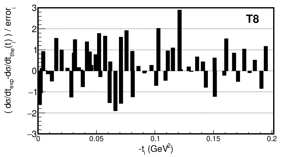
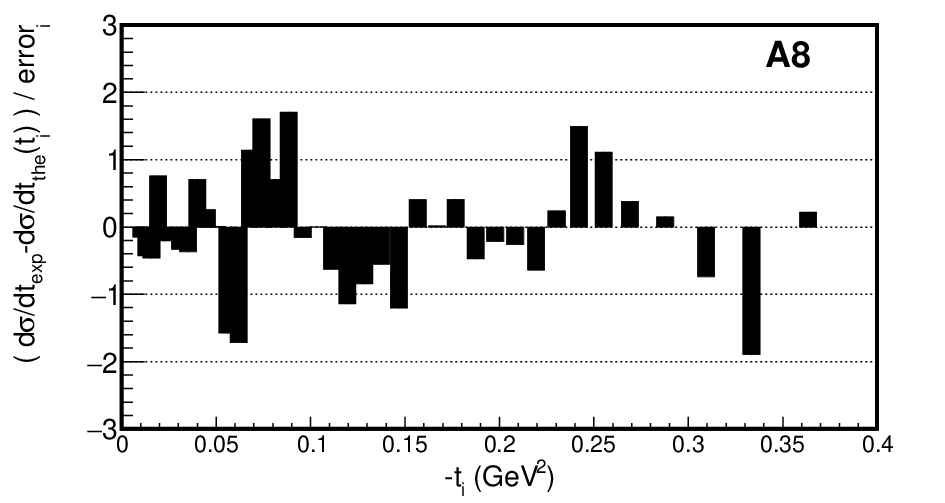
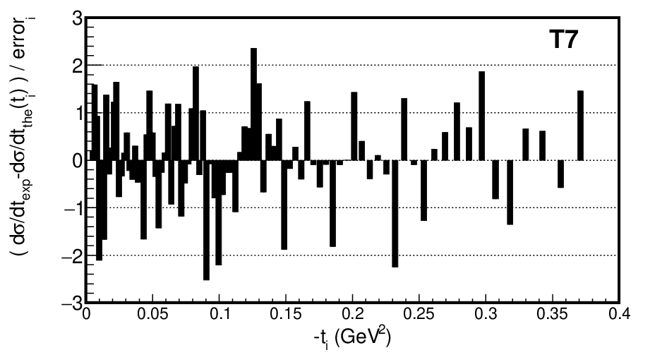
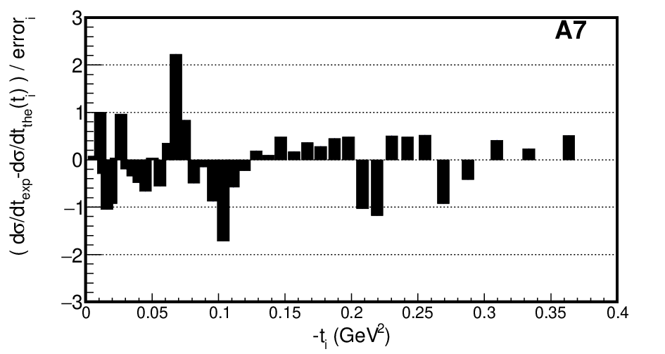
The regularity on the values of is remarkable. The zero of the real part determined by the parameters and is associated with the predicted zero of the theorem by A. Martin [5]. We see that the position of the zero is stable in all experiments and in Table 4 we observe agreement at GeV2 within the statistical errors. In terms of amplitudes we observe that the position of the zero together with the magnitude of determines the structure shown in Fig. 2. The existence of this zero is very important for the superposition of the real and imaginary parts that controls the detailed structure of in the low region.
Finally, as a general remark we observe that total cross sections maintain that Totem values are higher than Atlas by 4-6 mb, and the numbers remain stable in all Conditions studied. Another general remark is that differences in the results obtained with the two assumptions for the Coulomb phase are relevant only for T8 that has experimental points for very small . It may be fortuitous, but we observe that is smaller when the phase is put at .
The difficulty in the determination of may be due to the Coulomb-Nuclear interference. The distribution of electric charge in the proton determined by electromagnetic scattering at low energies () may be not realistic for high energy hadronic scattering. In Appendix A we show that with expanded proton size (as it may be the case at high energies) the Coulomb phase decreases. We see that the problem of the Coulomb interference in elastic pp scattering still has open questions.
V Conclusions
In this work we study the properties of the amplitudes in pp elastic scattering analysing experimental data at the LHC center-of-mass energies 7 and 8 TeV, based on a model for the complex amplitude, with explicit real and imaginary parts, each containing an exponential slope and a linear factor to account for the existence of a zero. The zero of the real part, close to the origin, corresponds to Martin’s Theorem, and the zero of the imaginary part anticipates the dip in the differential cross section that occurs beyond the range of the available data under study.
Our study shows that the real amplitude plays crucial role in the description of the differential cross section in the forward region. Interference with the Coulomb interaction is properly accounted for, and use is made of information from external sources, such as dispersion relations and predictions for the imaginary zero obtained in studies of full-t behaviour of the differential cross section [7, 6]. We organize the analysis under four conditions, according to the specifications of the parameters with values fixed in each case. Comparison is made of the results obtained for the four experimental measurements. We obtain the results shown in Table 4 that we believe to be a good representation of the experimental data of Table 1.
| Fixed Quantities : , (8 TeV) [7], (7 TeV) [6] | |||||||||||
| N | ndf | ||||||||||
| (mb) | |||||||||||
| T8 | 60 | 102.400.15 | 0.14 (fix) | 15.270.39 | 21.150.39 | -3.690.15 | -2.16 (fix) | -0.0380.002 | 19.590.39 | 73.862.18 | 69.2/56 |
| A8 | 39 | 96.820.11 | 0.14 (fix) | 15.260.06 | 21.650.24 | -3.690.12 | -2.16 (fix) | -0.0380.001 | 20.030.14 | 74.361.73 | 29.97/35 |
| T7 | 87 | 99.800.21 | 0.14 (fix) | 15.710.14 | 24.260.47 | -4.240.31 | -2.14 (fix) | -0.0330.002 | 19.990.14 | 84.834.45 | 95.08/83 |
| T7 | 87+17 | 99.440.14 | 0.14 (fix) | 15.440.07 | 22.620.19 | -3.490.13 | -2.14 (fix) | -0.0400.002 | 19.720.07 | 72.481.87 | 203.5/100 |
| A7 | 40 | 95.750.16 | 0.14 (fix) | 15.230.11 | 21.860.44 | -3.990.22 | -2.14 (fix) | -0.0350.002 | 19.510.11 | 78.863.17 | 27.33/36 |
Assuming at high energies, dispersion relations give , and we know that the position of the first real zero [7] behaves like . From Eq.(11) it then follows that increases like at high energies. With in , from Table 4 we obtain . Future precise measurements in LHC at 13 TeV may be investigated with this purpose. Our present work predicts that the zero at TeV is at .
The quantity is related with the scaling variable introduced by J. Dias de Deus [18] connecting and dependences in the amplitudes at high energies and small . A. Martin [19] uses the same idea of a scaling variable, writing an equation for the real part using crossing symmetric scattering amplitudes of a complex variable, valid in a forward range. The proposed ratio is
| (17) |
where is a damping function, with the implicit existence of a real zero. The form of determines the properties of the real zero [20]. that is found in the analysis of the data. This may be a clue for the introduction of explicit crossing symmetry and analyticity in our phenomenological treatment of the data.
Other models [8] also deal with the position of the real zero, discussing different analytical forms for the amplitudes, and it would be interesting to have their predictions for the amplitudes in the forward range.
In Appendix B we investigate the behaviour the amplitudes in -space for a geometric insight of the scattering process. We find that although our amplitudes never violate Eq.(46) up to 8 TeV at LHC, the differential cross sections in -space are all monotonically decreasing functions in . This means that our amplitudes do not indicate any signal for peripheral dominant elastic scattering process. However, in an analysis of T8 a dominance of the square of the real amplitude in -space Ref. [21] interpreted as a peripheral behaviour. To settle this interesting question, data at larger are required.
In non-perturbative QCD, in several instances, the proton appears as a structure with expanding size as the energy increases [22], with varied mechanisms, as distribution of valence quarks in a cloud around a core, modifications in QCD vacuum in the region of the colliding particles, and so on. Together with the evolution of the proton hadronic size, its electromagnetic properties, as they appear in high energy collisions, may change also. A linear increase in is a usual assumption for the effective proton radius, and the form factor parameter would then be reduced by about 1/2, corresponding to increase of about 40 % in proton radius. In Appendix A we calculate the interference phase with this example.
We expect that future data in pp elastic scattering at 13 TeV and higher energies will have high quality covering a wide range to allow determination of the properties of the real and imaginary amplitudes in pp elastic scattering, including studies of the amplitudes up to the perturbative tail of large . Hopefully the experimental groups will receive the necessary support and encouragement for this effort.
Acknowledgements.
TK, EF and AKK thank INCT-FNA Proc.No. 464898/2014-5 for the support. The authors wish to thank the Brazilian agencies CNPq, CAPES, PRONEX and FAPERJ for financial support. AKK thanks Jiri Prochazka for stimulating discussions during EDSBlois 2017.Appendix A Coulomb Phase
Abstract We study the phase of t scattering according to the formulation based on superposition of nuclear and Coulomb interactions in the eikonal formalism. The expressions for the phase accounting for the structure of the real and imaginary parts of the amplitude are obtained.
The Coulomb interference in pp elastic scattering is very important for the analysis of LHC experiments, where the properties of the amplitudes are investigated. The phase of the quantum interference between Coulomb and nuclear interactions was studied by several authors [13, 14, 6, 12, 15, 16]. A first approach for the so called Coulomb phase, is the point-like (pure Coulomb) phase, derived by West Yennie [13] calculated in the context of quantum field theory, considering the nuclear imaginary and real amplitudes with the same t-dependence and a proton with zero radius. The results for pointlike proton [13] have been generalized [6] allowing different slopes for the real and imaginary nuclear amplitudes. A second approach is the form-factor phase, which considers an eikonal treatment for the superposition of amplitudes and a geometrical size with a form factor for the proton structure [14, 12, 15].
The expression for the phase depends on the analytical structure of the real and imaginary parts of the nuclear amplitude. Here we derive in the same eikonal formalism an expression for the Coulomb interference phase appropriate for forward scattering amplitude with dependence of the form
| (18) |
that is assumed to be realistic for the description of data for high energy, satisfying expected properties concerning zeros, signs and magnitudes of the amplitudes in the forward range. To have systematic symmetry in the notation, we write for the usual, parameter, and .
The usual dipole electromagnetic form factor is
| (19) |
with . To simplify calculations, we may alternatively use the Gaussian representation for the form factor
| (20) |
trusting that differences in results for the phases are unimportant, as confirmed by Cahn [14].
The Coulomb amplitude for pp scattering, written
| (21) |
enters the Coulomb-Nuclear-Interference (CNI) in the form
| (22) |
with normalization defined by
| (23) |
We start from the exact expression for the phase
| (24) |
the signs corresponding to the systems.
Cahn has considered the approximation
| (25) |
justifying that the momentum transfer scale is much smaller than the inverse size of the proton. This is a very strong assumption, that should be tested in specific cases. Following the suggestion, Eq. (24) becomes
| (26) |
where for simplicity we use the variable instead of . As a generalization with respect to Cahn’s calculation, we take for the nuclear amplitude the same expression in Eq. (18), namely
Then we need to evaluate integrals
| (27) |
where we have used the definition
with .
The results of the integrations (N=0,1,2) are
| (28) |
where is the Euler Gamma constant. The phase is then written
| (29) |
with real and imaginary parts respectively
| (30) |
and
| (31) |
Eqs. (30) and (31) are our final results for the phase calculated with form factors, in a generalization of the work by Cahn [14], assuming more complete structures for the real and imaginary parts of the scattering amplitude. It may be of practical usefulness to define
| (32) |
and
| (33) |
and then write
| (34) |
and
| (35) |
It must be observed that in these expressions , and have compatible units, as and . The result is simple: in the real part the dependence is purely linear in , the imaginary part is very small constant, and there is no explicit energy dependence.
In the simplified case
we obtain Cahn’s original form.
The real and imaginary parts of the phase are plotted in Fig. 8 with an example of values for the parameters.

In the figure we plot also (dot-dashed) a line representing the real part of the phase calculated for a larger proton, with .
Appendix B -space properties
Let be the dimensionless Fourier transform of the amplitude in Eqs. (4, 6) with respect to the momentum transfer. Writing
| (36) |
we have
| (37) |
and
| (38) |
In Fig.(9) we show at = 8 TeV as function of for T8 and A8.

In Fig. (9), we show the general tendency of the scattering amplitudes in the two measurements, that differ by only a few %. Note that the magnitude of real parts become comparable, and even greater than the imaginary parts for large values. Such a behaviour is not the case for lower energies. The similar behaviour is similar for the 7 TeV datasets.
To investigate in more detail the significance of the behaviour of the real part dominance in the peripheral region, let us introduce the eikonal representation of the space amplitude as ([7])
| (39) |
and the so-called space differential cross sections (profile functions) are
| (40) |
| (41) |
| (42) |
where and .
The above -space representations of the differential cross sections offer a geometric view of the pp interactions, although such interpretation should be taken with care because they are not physical observables. From the unitarity condition of the scattering amplitude, we must have , and . We have which implies . Thus, in this region, taking up to the leading orders in and respectively, we obtain
| (43) |
| (44) |
and
| (45) |
From the above, it is clear that in the domain where (that is, where the Born approximation is valid), the inelastic part comes totally from whereas the elastic contribution may exceed the inelastic one if
| (46) |
Thus the appearance of the peripheral domain where may indicate that the contribution of elastic scattering is going to be significant in the peripheral region, and even can be dominant if relation (46) is satisfied. If this situation happens, the scattering is basically elastic and a possible candidate that we can imagine in such situation is the elastic scattering channel due to virtual pion exchange.
In the model of M. M. Islam [23] the proton structure is described by three layers: the first within a radius of fm contains three valence quarks (exchange of small-x gluons), the second layer is a shell of baryonic charge fm (responsible for exchanges) and the outer layer is the condensate which dominates diffractive scattering and is the same for both proton and anti-proton. However the polarization induced by the inner shells change the distribution of charges around the proton from pp to pp̄. This re-distribution affects the amplitudes and creates a contribution which is energy dependent. In other words this can be interpreted as a change in the proton electromagnetic form factor. On the other hand, in the present analysis, the relation (46) is far from be satisfied for all datasets, for and TeV. That is, there appear no elastic scattering dominant outer shell at these and lower energies.
Below, we show the plots of various -space differential cross sections using the amplitudes obtained in the present analysis. Note that the corresponding -space amplitude satisfies the unitarity condition mentioned before, satisfying

As seen from these figures, for all results, although the real part amplitude becomes dominant over the imaginary part in the peripheral region, the inelastic contribution is totally dominant over the elastic contribution at these energies (7 and 8 TeV). On the other hand, if such a tendency of increase of the real part continues for much higher energies and eventually becomes dominant compared to the imaginary part for the peripheral region, then the contribution from the elastic contribution becomes larger and the ratio may increase, approaching the black-disk limit. If this scenario happens and this is due to the elastic scattering by pion cloud, then we would expect that the Froissart bound might be saturated. However, as far as the data indicate the above speculative scenario where the real part becomes dominant, it is very unlikely for few hundred TeV energies, even considering the sensibilities and uncertainties in the determination of real and imaginary amplitudes. The question of asymptotic properties for asymptotic energies, we require more careful analysis of the real and imaginary amplitudes only for the forward region but also for the larger values.
References
- [1] G. Antchev et al. (TOTEM Coll.), Eurphys. Lett. 101, 21002 (2013).
- [2] G. Aad et al. (ATLAS Collaboration), Nucl. Phys. B 889, 486 (2014).
- [3] G. Antchev et al. (TOTEM Coll.), Eur. Phys. J. C. 16, 661 (2016) ; Nucl. Phys. B 899, 527 (2015).
- [4] G. Aad et al. (ATLAS Collaboration), Phys. Lett. B 761 158 (2016).
- [5] A. Martin, Phys. Lett. B 404, 137 (1997).
- [6] A. Kendi Kohara, E. Ferreira, and T. Kodama, Eur. Phys. J. C 73, 2326 (2013).
- [7] A. K. Kohara, E. Ferreira, and T. Kodama, Eur. Phys. J. C 74, 3175 (2014) .
- [8] C. Bourrely, J. Soffer, and T. T. Wu, Nucl. Phys. B 247, 15 (1984); Phys. Rev. Lett. 54, 757 (1985); Phys. Lett. B 196, 237 (1987); A. K. Kohara, E. Ferreira, and T. Kodama, Phys. Rev. D 87, 054024 (2013); V. A. Petrov, E. Predazzi and A. V. Prokudin , Eur. Phys. J. C 28, 525 (2003); O. V. Selyugin , Phys. Rev. D 60, 074028 (1999); M. M. Islam, R. J. Luddy, and A. V. Prokudin, Mod. Phys. Lett. A 18, 743 (2003).
- [9] E. Ferreira, Int. Jour. Mod. Phys. E 16, 2893 (2007).
- [10] C. Patrign et al. (Particle Data Group), Chinese Physics C 40, 100001 (2016).
- [11] J. R. Cudell et al. (COMPETE Collaboration), Phys. Rev. Lett. 89, 201801 (2002)
- [12] V. Kundrát and M. Lokajicek, Phys. Lett. B 611, 102 (2005); V.Kundrát, M.Lokajicek and I. Vrococ, Phys. Lett. B 656, 182 (2007).
- [13] G. B. West and D. Yennie , Ann. of Phys. 3, 190 (1958); Phys. Rev. 172, 5 (1968)
- [14] R. Cahn, Zeit. Phys. C 15, 253 (1982) .
- [15] O. V. Selyugin , Phys. Rev. D 60, 074028 (1999).
- [16] V. A. Petrov, E. Predazzi and A. V. Prokudin , Eur. Phys. J. C 28, 525 (2003) .
- [17] R. Brun and F. Rademakers, Nucl. Instrum. Meth. A 389, 81 (1997).
- [18] J. D. Deus, Nuc. Phys. B 59, 231 (1973) ; Phys. Lett. B 718, 1571 (2013).
- [19] A. Martin, Lett. Nuovo Cim. 7, 811 (1973) .
- [20] I. M. Dremin, arXiv:1204.1914 [hep-ph] .
- [21] J. Prochazka and V. Kundrat, arxiv.org/pdf/1606.09479 (2016).
- [22] J. Dias de Deus and P. Kroll, Nuovo Cimento A 37, 67 (1977); Acta Phys. Pol. B 9, 157 (1978); J. Phys. G 9, L81 (1983); P. Kroll, Z. Phys. C 15, 67 (1982); T. T. Chou and C. N. Yang, Phys. Rev. 170, 1591 (1968); Phys. Rev. D 19, 3268 (1979); Phys. Lett. B 128, 457 (1983); Phys. Lett. B 244, 113 (1990) ; B. Povh and J. Hüfner, Phys. Rev. Lett. 58, 1612 (1987); Phys. Lett. B 215, 722 (1988); Phys. Lett. B 245, 653 (1990); Phys. Rev. D 46, 990 (1992); Z. Phys. C 63, 631 (1994); E. Ferreira and F. Pereira, Phys. Rev. D 55, 130 (1997); Phys. Rev. D 56, 179 (1997).
- [23] M.M. Islam and R.J. Luddy, Acta Phys. Pol. B Proc. Sup., 8 4 (2015).