跳到论文正文
W Papers独立论文阅读器 arXiv:1709.05528 论文正文 计算阅读时间 · 0%
引用这篇论文根据当前论文元数据生成,正式投稿前建议核对。


License: arXiv.org perpetual non-exclusive license
arXiv:1709.05528v2 [eess.SY] 03 Mar 2018

Convergence Analysis and Design of ADMM via Switched
Control Theory: Supplementary Material

Jun Li Affiliation: Department of Electrical and Computer Engineering, Northeastern University, Boston, MA, USA. Correspondence to: junl.mldl@gmail.com    Hongfu Liu Affiliation: Department of Electrical and Computer Engineering, Northeastern University, Boston, MA, USA. Correspondence to: liu.hongf@husky.neu.edu    Yue Wu Affiliation: Department of Electrical and Computer Engineering, Northeastern University, Boston, MA, USA. Correspondence to: yuewu@ece.neu.edu    Yun Fu Affiliation: Department of Electrical and Computer Engineering, Northeastern University, Boston, MA, USA. Correspondence to: yunfu@ece.neu.edu
Abstract

We consider three challenges in multi-block Alternating Direction Method of Multipliers (ADMM): building convergence conditions for ADMM with any block (variable) sequence, finding available block sequences to be fit for ADMM, and designing useful parameter controllers for ADMM with unfixed parameters. To address these challenges, we develop a switched control framework for studying multi-block ADMM. First, since ADMM recursively and alternately updates the block-variables, it is converted into a discrete-time switched dynamical system. Second, we study exponential stability and stabilizability of the switched system for linear convergence analysis and design of ADMM by employing switched Lyapunov functions. Moreover, linear matrix inequalities conditions are proposed to ensure convergence of ADMM under arbitrary sequence, to find convergent sequences, and to design the fixed parameters. These conditions are checked and solved by employing semidefinite programming.

Keywords: 
Machine Learning, ICML
††affiliationnotice: Equal contribution

1 Introduction

The alternating direction method of multipliers (ADMM) is usually applied to solve the following convex minimization problem with N≥3N\geq 3 blocks of variables {xi}i=1N\{\textbf{x}_{i}\}_{i=1}^{N}:

min⁡∑i=1Nxi∈𝒳i,1≤i≤N⁡fi​(xi)​s.t.​∑i=1NAi​xi=q,\displaystyle\begin{array}[]{l@{}l}\min_{\textbf{x}_{i}\in\mathcal{X}_{i},1\leq i\leq N}\ \sum_{i=1}^{N}f_{i}(\textbf{x}_{i})\ \mbox{s.t.}\ \sum_{i=1}^{N}\textbf{A}_{i}\textbf{x}_{i}=\textbf{q},\end{array}

where Ai∈ℝm×ni\textbf{A}_{i}\in\mathbb{R}^{m\times n_{i}}, q∈ℝm\textbf{q}\in\mathbb{R}^{m}, 𝒳i⊂ℝni\mathcal{X}_{i}\subset\mathbb{R}^{n_{i}} are closed convex sets, and fi:ℝni→ℝ¯=ℝ​⋃{+∞}f_{i}:\mathbb{R}^{n_{i}}\rightarrow\overline{\mathbb{R}}=\mathbb{R}\bigcup\{+\infty\} are closed proper convex functions. After the ADMM was originally proposed in the early 1970s (Glowinski & Marrocco, 1975; Gabay & Mercier, 1976), it has received increasing attention in wide applications, such as in machine learning, computer vision and signal processing (Chang et al., 2016; Hong et al., 2016; Wang et al., 2017). Actually, the performance of these applications heavily depends on the convergence (at least acceptable accuracy) of ADMMs. It is well-known that the convergence of two-block ADMM has been proved in literature (Eckstein & Bertsekas, 1992). When N≥3N\geq 3, however, the systematic convergence analysis of multi-block ADMM has been void for a long time.

Recently, global (linear) convergence and sublinear convergence of multi-block ADMM have been proved under the condition that functions are (strongly) convex and the penalty factor is restricted to a certain region (Han & Yuan, 2012; Lin et al., 2015b; Sun et al., 2015; Lin et al., 2015a; Lin et al., 2016; Li et al., 2016; Xu et al., 2017; Lu et al., 2017). Moreover, ADMMs are also extended into parallel or distributed manners by using a Jacobi-type scheme (Lu et al., 2016; Deng et al., 2017). However, it is still unclear to systematically study multi-block ADMMs due to the following disadvantages. First, since these proofs are designed as an algorithm-by-algorithm basis (Lessard et al., 2016), it lacks a unified framework to analyze the convergence problem of multi-block ADMM. Second, most of multi-block ADMM only consider a persistent block sequence (i.e., x1,x2⋯,xN\textbf{x}_{1},\textbf{x}_{2}\cdots,\textbf{x}_{N}). This is conservative because it often leads to divergent algorithms. Third, ADMMs with unfixed parameters are usually divergent. In practice, it needs an effective method to design the fixed parameters. Forth, two-block ADMM is analyzed by adopting the integral quadratic constraint (IQC) framework (Megretski & Rantzer, 1997) from control theory, and formulating linear matrix equalities (LMIs) conditions for its linear convergence (Nishihara et al., 2015). However, it only limits to the simple two-block ADMM. To study multi-block ADMM intensively, therefore, we focus on the following three basic challenges.

Challenge 1: Build sufficient conditions to guarantee that multi-block ADMM is convergent for any block sequence. For the convergence problem, the first essential question is whether multi-block ADMM is convergent when there is no restriction on the block sequences. This basic challenge is called convergence under arbitrary (block) sequence.

Challenge 2: Find block sequences that makes multi-block ADMM convergent. The arbitrary sequence is too strict to preserve the convergence of multi-block ADMM. However, it may be convergent under restricted block sequences. This leads us to find suitable sequences between the block-variables to ensure the convergence of multi-block ADMM, instead of the arbitrary sequence.

Challenge 3: Design fixed parameters that drive divergent multi-block ADMM to be convergent. In fact, it is still possible to difficultly find a convergent block sequence in the challenge 2 due to the unsuitable parameters (e.g., penalty factors, damping factors, and matrices Ai\textbf{A}_{i} in Eq. (1)). For example, a counter example is constructed to show the failure of three-block ADMM (Chen et al., 2016). This arouses the third basic challenge that how to construct fixed parameters to drive divergent ADMM to have a convergent trajectory.

In general, multi-block ADMM decomposes the convex problem (1) into NN smaller subproblems for the block-variables xi\textbf{x}_{i}. Specially, it alternately orchestrates switching between these subproblems, which are solved by recursively updating the corresponding block-variables. Clearly, this orchestration constitutes a block-variable switching sequence on the NN subproblems. Moreover, following the transformation of two-block ADMM (Nishihara et al., 2015), each subproblem can be easily converted into a discrete-time dynamical subsystem. Thus, multi-block ADMM can be viewed as a discrete-time switched dynamical system that consists of NN different subsystems and a switching rule between these subsystems (Liberzon et al., 1999). In particular, the related parameters are correspondingly changed into the weight matrices of the subsystems.

Based on above discussions, therefore, the three basic challenges of multi-block ADMM can be solved by analyzing the switched system with the switched control theory (Lin & Antsaklis, 2009). Challenge 1 is translated into building sufficient conditions for the stability of the switched system under arbitrary switching. Some LMIs conditions for the related parameters are constructed in subsection 4.1. Challenge 2 becomes to search for switching pathes on these conditions to ensure the stability of the switched system under suitable switching. A recursive search Algorithm 1 is proposed in subsection 4.2. Challenge 3 turns to analyze the stabilizability of the switched system by designing feedback controller (regulative parameter matrices). Some controllers are developed in subsection 4.3. This provides a practical approach to design the fixed parameters for multi-block ADMM instances. Overall, our main contributions are summarized as follows:

  • •

    To the best of our knowledge, we are the first to convert multi-block ADMM into a discrete-time switched dynamical system. The convergence of multi-block ADMM is analyzed and controlled by studying the stability and stabilizability of this switched system.

  • •

    We propose efficient LMIs conditions to ensure the linear convergence of multi-block ADMM under arbitrary sequence, and search for the convergent sequences on the block-variables. The size of LMIs scales with the number of the blocks.

  • •

    We design useful parameter controllers to drive multi-block ADMM to be convergent. These controllers are used to construct linear equality constraints for multi-block ADMM, and adjust the directions of trajectories of the variables in the feasible region. It is worth noting that the counter example (Chen et al., 2016) can converge by designing a parameter controller.

2 Preliminaries

In this section, we give some notations, and introduce the classical ADMMs and the discrete-time switched system.

2.1 Notations

We give some notations as follows. An index set ℐ\mathcal{I} is denoted by {1,⋯,N+1}\{1,\cdots,N\hskip-2.84544pt+\hskip-2.84544pt1\}. A P-norm of y, ‖y‖P\|\textbf{y}\|_{\textbf{P}}, is denoted as yT​Py\sqrt{\textbf{y}^{T}\textbf{P}\textbf{y}}. The condition number of A is denoted as κA=σ1​(A)/σp​(A)\kappa_{\textbf{A}}=\sigma_{1}(\textbf{A})/\sigma_{p}(\textbf{A}), where σ1​(A)\sigma_{1}(\textbf{A}) and σp​(A)\sigma_{p}(\textbf{A}) denote the largest and smallest singular values of the matrix A. The Hadamard product of matrices A and B is denoted as A∘B\textbf{A}\circ\textbf{B}. We denote a m×mm\times m identity matrix and zero matrix by Im\textbf{I}_{m} and 0m\textbf{0}_{m}, respectively. A m×nm\times n all ones matrix is denoted as Jm×n\textbf{J}_{m\times n}. The ii-th m×mm\times m identity matrix with ones on the ii-th main diagonal and zeros elsewhere is denoted as 𝕀mi=diag​(0,⋯,1,⋯,0)\mathbb{I}_{m}^{i}=\mbox{diag}(0,\cdots,1,\cdots,0). We denote the Kronecker product of matrices A and B by A⊗B\textbf{A}\otimes\textbf{B}. We denote a symmetric matrix (XYYTZ)\left(\hskip-5.69046pt\begin{array}[]{cc}\textbf{X}&\textbf{Y}\\ \textbf{Y}^{T}&\textbf{Z}\\ \end{array}\hskip-5.69046pt\right) by (XY⋆Z)\left(\hskip-5.69046pt\begin{array}[]{cc}\textbf{X}&\textbf{Y}\\ \star&\textbf{Z}\\ \end{array}\hskip-5.69046pt\right). A positive-definite matrix A is denoted as A>0\textbf{A}>0. In general, we let ∇f\nabla f denote the gradient of ff if it is convex and differentiable, and let ∂f\partial f denote the subdifferential of ff if it is convex. Suppose that the functions fi:ℝni→ℝ¯=ℝ​⋃{+∞}f_{i}:\mathbb{R}^{n_{i}}\rightarrow\overline{\mathbb{R}}=\mathbb{R}\bigcup\{+\infty\} satisfy the following assumption.

Assumption 1. For any function fi​jf_{ij}, i=1,2,⋯,Ni=1,2,\cdots,N and j=1,2,⋯,nij=1,2,\cdots,n_{i}, there exist constants νi​j−\nu_{ij}^{-} and νi​j+\nu_{ij}^{+} such that

νi​j−≤𝔣i​j​(x1)−𝔣i​j​(x2)x1−x2≤νi​j+,∀x1,x2,x1≠x2,\displaystyle\nu_{ij}^{-}\leq\frac{\mathfrak{f}_{ij}(x_{1})-\mathfrak{f}_{ij}(x_{2})}{x_{1}-x_{2}}\leq\nu_{ij}^{+},\ \forall x_{1},x_{2},x_{1}\neq x_{2}, (2)

where 𝔣i​j​(⋅)\mathfrak{f}_{ij}(\cdot) is the gradient or subgradient of fi​j​(⋅)f_{ij}(\cdot). For example, 𝔣i​j​(⋅)←{=∇fi​j​(⋅),fi​j is strong convex,∈∂fi​j​(⋅),fi​j is convex.\mathfrak{f}_{ij}(\cdot)\leftarrow\left\{\begin{array}[]{ll}=\nabla f_{ij}(\cdot),&\hbox{$f_{ij}$ is strong convex,}\\ \in\partial f_{ij}(\cdot),&\hbox{$f_{ij}$ is convex.}\end{array}\right..

2.2 Classical ADMMs

To solve the problem (1), we consider the augmented Lagrangian function:

ℒβ​(x1,⋯,xi,⋯,xN,λ)=∑i=1Nfi​(xi)+λT​(∑i=1NAi​xi−q)+β2​‖∑i=1NAi​xi−q‖22,\begin{array}[]{l@{}l}&\mathcal{L}_{\beta}(\textbf{x}_{1},\cdots,\textbf{x}_{i},\cdots,\textbf{x}_{N},\lambda)=\sum_{i=1}^{N}f_{i}(\textbf{x}_{i})\\ &\ \ \ \ \ \ \ \ \ \ \ \ \ \ \ +\lambda^{T}(\sum_{i=1}^{N}\textbf{A}_{i}\textbf{x}_{i}-\textbf{q})+\frac{\beta}{2}\|\sum_{i=1}^{N}\textbf{A}_{i}\textbf{x}_{i}-\textbf{q}\|_{2}^{2},\end{array}

with the Lagrange multiplier λ∈ℝm\lambda\in\mathbb{R}^{m} and a penalty parameter β>0\beta>0. Roughly, most of ADMMs can be categorized into Gauss-Seidel ADMM and Jacobian ADMM. The Gauss-Seidel ADMMs update a variable xi\textbf{x}_{i} by fixing others as their latest versions in a sequential manner (Boyd et al., 2011), while the Jacobian ADMMs update all the NN block-variables xi\textbf{x}_{i} (1≤i≤N)(1\leq i\leq N) in a parallel manner (Deng et al., 2017). The iterative scheme of the Gauss-Seidel ADMM (GS-ADMM) is outlined below: for 1≤i≤N1\leq i\leq N,

{xik+1=arg​minxi​fi​(xi)+β2|∑j<iAj​xjk+1+Aixi+∑j>iAjxjk+β−1λk−q∥22+12​‖xi−xik‖Si2,λk+1=λk−γ​β​(∑j=1NAj​xjk+1−q),\displaystyle\left\{\hskip-5.69046pt\begin{array}[]{l@{}l}\textbf{x}_{i}^{k+1}=&\mbox{arg}\min_{\textbf{x}_{i}}f_{i}(\textbf{x}_{i})+\frac{\beta}{2}\|\sum_{j<i}\textbf{A}_{j}\textbf{x}_{j}^{k+1}\\ &+\textbf{A}_{i}\textbf{x}_{i}+\sum_{j>i}\textbf{A}_{j}\textbf{x}_{j}^{k}+\beta^{-1}\lambda^{k}-\textbf{q}\|_{2}^{2}\\ &+\frac{1}{2}\|\textbf{x}_{i}-\textbf{x}_{i}^{k}\|_{\textbf{S}_{i}}^{2},\\ \lambda^{k+1}=&\lambda^{k}-\gamma\beta(\sum_{j=1}^{N}\textbf{A}_{j}\textbf{x}_{j}^{k+1}-\textbf{q}),\end{array}\right.

and a general Jacobian ADMM, Proximal-Jacobian ADMM (PJ-ADMM) (Deng et al., 2017), updates the variable xi\textbf{x}_{i} in parallel by: for 1≤i≤N1\leq i\leq N,

{xik+1=arg​minxi​fi​(xi)+β2|∑j=1,≠iNAj​xjk+Aixi+β−1λk−q∥22+12∥xi−xik∥Si2,λk+1=λk−γ​β​(∑j=1NAj​xjk−q),\displaystyle\left\{\hskip-5.69046pt\begin{array}[]{l@{}l}\textbf{x}_{i}^{k+1}=&\mbox{arg}\min_{\textbf{x}_{i}}f_{i}(\textbf{x}_{i})+\frac{\beta}{2}\|\sum_{j=1,\neq i}^{N}\textbf{A}_{j}\textbf{x}_{j}^{k}\\ &+\textbf{A}_{i}\textbf{x}_{i}+\beta^{-1}\lambda^{k}-\textbf{q}\|_{2}^{2}+\frac{1}{2}\|\textbf{x}_{i}-\textbf{x}_{i}^{k}\|_{\textbf{S}_{i}}^{2},\\ \lambda^{k+1}=&\lambda^{k}-\gamma\beta(\sum_{j=1}^{N}\textbf{A}_{j}\textbf{x}_{j}^{k}-\textbf{q}),\end{array}\right.

where ‖xi‖Si2=xiT​Si​xi\|\textbf{x}_{i}\|_{\textbf{S}_{i}}^{2}=\textbf{x}_{i}^{T}\textbf{S}_{i}\textbf{x}_{i}, Si=αi​I−β​AiT​Ai\textbf{S}_{i}=\alpha_{i}\textbf{I}-\beta\textbf{A}_{i}^{T}\textbf{A}_{i} (αi>0)(\alpha_{i}>0) and γ>0\gamma>0 is a damping parameter. When Si=0\textbf{S}_{i}=0, the ADMMs (2.2) and (2.2) can be rewritten as the standard ADMM (Deng & Yin, 2016). When Si=αi​I\textbf{S}_{i}=\alpha_{i}\textbf{I}, it corresponds to the standard proximal method (Parikh & Boyd, 2014). The convergent point of (2.2) and (2.2) is denoted as x⋆=((x1⋆)T,⋯,(xN⋆)T,(λ⋆)T)T\textbf{x}^{\star}=((\textbf{x}_{1}^{\star})^{T},\cdots,(\textbf{x}_{N}^{\star})^{T},(\lambda^{\star})^{T})^{T}.

2.3 Discrete-time Switched System

Consider a discrete-time switched dynamical system

ξt+1=ℬi​ξt+𝒞i​𝒢​(ξt)+𝒟i​ωt+ℰi​ϕ,i∈ℐ,\displaystyle\xi^{t+1}=\mathcal{B}_{i}\xi^{t}+\mathcal{C}_{i}\mathcal{G}(\xi^{t})+\mathcal{D}_{i}\omega^{t}+\mathcal{E}_{i}\phi,\ \ i\in\mathcal{I}, (10)

with an initialized system state ξ0=ϕξ​(0)\xi^{0}=\phi_{\xi}(0) and a control input ω0=ϕω​(0)\omega^{0}=\phi_{\omega}(0), where t∈ℤ+t\in\mathbb{Z}^{+}, ξt∈ℝnξ\xi^{t}\in\mathbb{R}^{n_{\xi}} is the state, ωt∈ℝnω\omega^{t}\in\mathbb{R}^{n_{\omega}} is the control input, ϕ\phi is the offset input, 𝒢⁡(⋅)\mathcal{G}(\cdot) is a nonlinear function vector, ℬi\mathcal{B}_{i} and 𝒞i∈ℝnξ×nξ\mathcal{C}_{i}\in\mathbb{R}^{n_{\xi}\times n_{\xi}} are the state transition matrices, and 𝒟i\mathcal{D}_{i} and ℰi∈ℝnξ×nω\mathcal{E}_{i}\in\mathbb{R}^{n_{\xi}\times n_{\omega}} are the control and offset input matrices. The system (10) is constructed for GS-ADMM, while ℐ={1}\mathcal{I}=\{1\}, it becomes a discrete-time dynamical system for PJ-ADMM.

Usually, it is popular to study the stability and stabilizability of the system (10) by employing switched quadratic Lyapunov functions (Daafouz et al., 2002). A global Lyapunov function is constructed as V⁡(t,ξt)=(ξt)T​Pσ⁡(t)​ξtV(t,\xi^{t})=(\xi^{t})^{T}\textbf{P}_{\sigma(t)}\xi^{t}, where σ⁡(t):ℤ+→ℐ\sigma(t):\mathbb{Z}^{+}\rightarrow\mathcal{I}. The index σ⁡(t)=i\sigma(t)=i is called the active ii-th subsystem at the discrete-time tt, and Pi\textbf{P}_{i} (i∈ℐ)(i\in\mathcal{I}) is a positive definite matrix for the Lyapunov function V⁡(t,ξt)V(t,\xi^{t}) of the ii-th subsystem. The stability conditions of the system (10) is provided by proving that the Lyapunov function V⁡(t,ξt)V(t,\xi^{t}) is decreasing. For better developing the switched Lyapunov function for the system (10) in the section 4, we introduce Finsler’s Lemma (Boyd et al., 1994) as follow.

Lemma 1 (Finsler’s Lemma): Let y∈ℝm\textbf{y}\in\mathbb{R}^{m}, P∈ℝn×n\textbf{P}\in\mathbb{R}^{n\times n} and H∈ℝn×m\textbf{H}\in\mathbb{R}^{n\times m} such that r​a​n​k​(H)=r<mrank(\textbf{H})=r<m and P=PT>0\textbf{P}=\textbf{P}^{T}>0. The following statements are equivalent:

    1) yT​Py<0\textbf{y}^{T}\textbf{P}\textbf{y}<0, ∀Hy=0,y≠0\forall\textbf{H}\textbf{y}=\textbf{0},\textbf{y}\neq\textbf{0}.

    2) ∃Y∈ℝm×n:P+YH+HT​YT<0\exists\textbf{Y}\in\mathbb{R}^{m\times n}:\textbf{P}+\textbf{YH}+\textbf{H}^{T}\textbf{Y}^{T}<0.

Finsler’s Lemma has been previously used in the control literature (Fang et al., 2004). Lemma 1 aims to eliminate design variables in matrix inequalities. In addition, the definition of global exponential stability for the dynamical system (10) is now given.

Definition 1. (Wu et al., 2010) The system (10) is said to be exponential stability, if there exist a constant χ>0\chi>0 and a factor 0<τ<10<\tau<1 such that

‖ξt−ξ⋆‖2≤χ​τt​‖ξ0−ξ⋆‖2.\displaystyle\|\xi^{t}-\xi^{\star}\|_{2}\leq\chi\tau^{t}\|\xi^{0}-\xi^{\star}\|_{2}. (11)

Definition 1 shows that when the ADMMs are written as the system (10), they will converge to ξ⋆\xi^{\star} if the system (10) is exponential stable. The system state sequence {ξt}\{\xi^{t}\} is said to converge linearly if 0<τ<10<\tau<1. When τ\tau (called convergence rate) is close to 00, ADMMs are fast convergent, and vice versa.

3 ADMMs as Switched Systems

We convert the classical ADDMs into dynamical systems in this section. GS-ADMM and PJ-ADMM are transformed into discrete-time switched dynamical systems in subsections 3.1 and 3.2, respectively. Before transforming ADMMs, we denote Bi\textbf{B}_{i}, Ci\textbf{C}_{i}, Di\textbf{D}_{i} and Ei\textbf{E}_{i} as follow:

Bi=\displaystyle\textbf{B}_{i}= 𝕀N+1i​B,Ci=𝕀N+1i​C,Di=𝕀N+1i​D,Ei=𝕀N+1i​E,\displaystyle\mathbb{I}_{N+1}^{i}\textbf{B},\ \textbf{C}_{i}=\mathbb{I}_{N+1}^{i}\textbf{C},\ \textbf{D}_{i}=\mathbb{I}_{N+1}^{i}\textbf{D},\ \textbf{E}_{i}=\mathbb{I}_{N+1}^{i}\textbf{E}, (12)
B=\displaystyle\textbf{B}= (1−βα^1−βα^1⋯−βα^1−1α^1−βα^21−βα^2⋯−βα^2−1α^2⋮⋮⋱⋮⋮−βα^N−βα^N⋯1−βα^N−1α^N−γ​β−γ​β⋯−γ​β0),α^i=αi‖Ai‖2,\displaystyle\left(\hskip-5.69046pt\begin{array}[]{ccccc}1-\frac{\beta}{\widehat{\alpha}_{1}}&-\frac{\beta}{\widehat{\alpha}_{1}}&\cdots&-\frac{\beta}{\widehat{\alpha}_{1}}&-\frac{1}{\widehat{\alpha}_{1}}\\ -\frac{\beta}{\widehat{\alpha}_{2}}&1-\frac{\beta}{\widehat{\alpha}_{2}}&\cdots&-\frac{\beta}{\widehat{\alpha}_{2}}&-\frac{1}{\widehat{\alpha}_{2}}\\ \vdots&\vdots&\ddots&\vdots&\vdots\\ -\frac{\beta}{\widehat{\alpha}_{N}}&-\frac{\beta}{\widehat{\alpha}_{N}}&\cdots&1-\frac{\beta}{\widehat{\alpha}_{N}}&-\frac{1}{\widehat{\alpha}_{N}}\\ -\gamma\beta&-\gamma\beta&\cdots&-\gamma\beta&0\\ \end{array}\hskip-5.69046pt\right),\ \ \widehat{\alpha}_{i}=\frac{\alpha_{i}}{\|\textbf{A}_{i}\|^{2}},
C=\displaystyle\textbf{C}= −diag(1α^1,⋯,1α^i,⋯1α^N,0),\displaystyle-\hbox{diag}\left(\frac{1}{\widehat{\alpha}_{1}},\cdots,\frac{1}{\widehat{\alpha}_{i}},\cdots\frac{1}{\widehat{\alpha}_{N}},0\right),
D=\displaystyle\textbf{D}= −diag​(βα^1,⋯,βα^i,⋯,βα^N,γ​β),E=D.\displaystyle-\hbox{diag}\left(\frac{\beta}{\widehat{\alpha}_{1}},\cdots,\frac{\beta}{\widehat{\alpha}_{i}},\cdots,\frac{\beta}{\widehat{\alpha}_{N}},\gamma\beta\right),\ \textbf{E}=\textbf{D}.

We cast ADMMs as a discrete-time switched dynamical system with state sequences {ξt}\{\xi^{t}\}, nonlinear functions 𝒢⁡(⋅)\mathcal{G}(\cdot), a control input ωt\omega^{t} and an offset input ϕ\phi.

State sequences {ξt}\{\xi^{t}\}. Denote ξik=Ai​xik\xi_{i}^{k}=\textbf{A}_{i}\textbf{x}_{i}^{k}. We define sequences {ξt∈ℝm⁡(N+1)}\{\xi^{t}\in\mathbb{R}^{m(N\hskip-1.42271pt+\hskip-1.42271pt1)}\} for GS-ADMM in sequential manner by

ξt=\displaystyle\xi^{t}= ((ξ1k+1)T,⋯,(ξi−1k+1)TCLOSE,\displaystyle\left((\xi_{1}^{k+1})^{T},\cdots,(\xi_{i-1}^{k+1})^{T},\right.
OPEN(ξik)T,(ξi+1k)T,⋯,(ξNk)T,(λk)T)T,\displaystyle\ \left.(\xi_{i}^{k})^{T},(\xi_{i+1}^{k})^{T},\cdots,(\xi_{N}^{k})^{T},(\lambda^{k})^{T}\right)^{T}, (18)

where t=k⁡(N+1)+i−1t=k(N\hskip-2.84544pt+\hskip-2.84544pt1)+i-1 and ii is the number of the updated variables in the kk-th iteration of GS-ADMM. Similar to GS-ADMM, we also define sequences {ξk∈ℝm⁡(N+1)}\{\xi^{k}\in\mathbb{R}^{m(N\hskip-1.42271pt+\hskip-1.42271pt1)}\} for PJ-ADMM in parallel manner by

ξk=((ξ1k)T,⋯,(ξik)T,⋯,(ξNk)T,(λk)T)T.\displaystyle\xi^{k}=\left((\xi_{1}^{k})^{T},\cdots,(\xi_{i}^{k})^{T},\cdots,(\xi_{N}^{k})^{T},(\lambda^{k})^{T}\right)^{T}. (19)

In this paper, ξk\xi^{k} is denoted as ξt\xi^{t} for consistency.

Nonlinear functions 𝒢⁡(⋅)\mathcal{G}(\cdot). Due to ξik=Ai​xik\xi_{i}^{k}=\textbf{A}_{i}\textbf{x}_{i}^{k}, gi:ℝm→ℝ¯g_{i}:\mathbb{R}^{m}\rightarrow\overline{\mathbb{R}}, where gi={fi∘Ai−1,fi is strong convex,fi∘Ai†+𝒮𝒳i,fi is convex.g_{i}=\left\{\begin{array}[]{ll}f_{i}\circ\textbf{A}_{i}^{-1},&\hbox{$f_{i}$ is strong convex,}\\ f_{i}\circ\textbf{A}_{i}^{{\dagger}}+\mathcal{S}_{\mathcal{X}_{i}},&\hbox{$f_{i}$ is convex.}\end{array}\right., Ai†\textbf{A}_{i}^{{\dagger}} is any left inverse of Ai\textbf{A}_{i}, and 𝒮𝒳i\mathcal{S}_{\mathcal{X}_{i}} is the {0,∞}\{0,\infty\}-indicator function. Based on the Assumption 1, a nonlinear function vector 𝒢:ℝd⁡(N+1)→ℝ¯\mathcal{G}:\mathbb{R}^{d(N+1)}\rightarrow\overline{\mathbb{R}} is denoted by

𝒢⁡(⋅)=(𝔤1​(⋅),⋯,𝔤N​(⋅),𝔤λ​(⋅))T⊗Jd×1,\displaystyle\mathcal{G}(\cdot)=\left(\mathfrak{g}_{1}(\cdot),\cdots,\mathfrak{g}_{N}(\cdot),\mathfrak{g}_{\lambda}(\cdot)\right)^{T}\otimes\textbf{J}_{d\times 1}, (20)

where 𝔤i:ℝ→ℝ¯\mathfrak{g}_{i}:\mathbb{R}\rightarrow\overline{\mathbb{R}} is used to simply represent a set {𝔤i​l}1≤l≤d\{\mathfrak{g}_{il}\}_{1\leq l\leq d}, 𝔤i​l​(⋅)\mathfrak{g}_{il}(\cdot) is the gradient or subgradient of gi​l​(⋅)g_{il}(\cdot), and 𝔤λ​(⋅)=0\mathfrak{g}_{\lambda}(\cdot)=0. Actually, 𝔤i​(⋅)\mathfrak{g}_{i}(\cdot) satisfies the following form:

μi−≤𝔤i​(x1)−𝔤i​(x2)x1−x2≤μi+,∀x1,x2,x1≠x2,\displaystyle\mu_{i}^{-}\leq\frac{\mathfrak{g}_{i}(x_{1})-\mathfrak{g}_{i}(x_{2})}{x_{1}-x_{2}}\leq\mu_{i}^{+},\ \ \ \forall x_{1},x_{2},x_{1}\neq x_{2},

where μi−=minj{νi​j−/σ12(Ai),νi​j−/σp2(Ai),1≤j≤ni}\mu_{i}^{-}=\min_{j}\{\nu_{ij}^{-}/\sigma_{1}^{2}(\textbf{A}_{i}),\nu_{ij}^{-}/\sigma_{p}^{2}(\textbf{A}_{i}),1\leq j\leq n_{i}\}, μi+=minj{νi​j+/σ12(Ai),νi​j+/σp2(Ai),1≤j≤ni}\mu_{i}^{+}=\min_{j}\{\nu_{ij}^{+}/\sigma_{1}^{2}(\textbf{A}_{i}),\nu_{ij}^{+}/\sigma_{p}^{2}(\textbf{A}_{i}),1\leq j\leq n_{i}\}, νi​j−\nu_{ij}^{-} and νi​j+\nu_{ij}^{+} are defined in (2). For presentation convenience in the following, we denote

F1=diag​(μ1−​μ1+,⋯,μN−​μN+,0),F2=diag​(μ1−+μ1+2,⋯,μN−+μN+2,0).\displaystyle\begin{array}[]{l@{}l}\textbf{F}_{1}&=\hbox{diag}\left(\mu_{1}^{-}\mu_{1}^{+},\cdots,\mu_{N}^{-}\mu_{N}^{+},0\right),\\ \textbf{F}_{2}&=\hbox{diag}\left(\frac{\mu_{1}^{-}+\mu_{1}^{+}}{2},\cdots,\frac{\mu_{N}^{-}+\mu_{N}^{+}}{2},0\right).\end{array}

The control input ωt\omega^{t}. In this paper, we aim also at designing the parameter feedback controllers,

ωt=𝒦i​ξt,i∈ℐ,\displaystyle\omega^{t}=\mathcal{K}_{i}\xi^{t},\ \ i\in\mathcal{I}, (23)

where 𝒦i=Ki⊗Id\mathcal{K}_{i}=\textbf{K}_{i}\otimes\textbf{I}_{d}, Ki=𝕀N+1i​K,\textbf{K}_{i}=\mathbb{I}_{N+1}^{i}\textbf{K}, K∈ℝ(N+1)×(N+1)\textbf{K}\in\mathbb{R}^{(N\hskip-1.42271pt+\hskip-1.42271pt1)\times(N\hskip-1.42271pt+\hskip-1.42271pt1)} is the control matrix. In subsection 4.3, our main objective is to obtain a suitable parameter matrix K for the system (10).

The offset input ϕ\phi. We consider the offset input ϕ=(qT,qT,⋯,0T)T∈ℝd⁡(N+1)×1\phi=\left(\textbf{q}^{T},\textbf{q}^{T},\cdots,\textbf{0}^{T}\right)^{T}\in\mathbb{R}^{d(\hskip-1.42271ptN+\hskip-1.42271pt1)\times 1}.

3.1 GS-ADMM (2.2) as a Switched System (24)

Based on above denoted variables and Assumption 1, GS-ADMM can be written as a discrete-time switched system in the following Proposition 1.

Proposition 1. Denote system states ξt\xi^{t} in (18) with activation function 𝒢⁡(⋅)\mathcal{G}(\cdot) in (20). GS-ADMM (2.2) is converted into the following switched system

ξt+1=\displaystyle\xi^{t+1}= (B^i⊗Id)​ξt+(Ci⊗Id)​𝒢​(ξt)\displaystyle(\widehat{\textbf{B}}_{i}\otimes\textbf{I}_{d})\xi^{t}+(\textbf{C}_{i}\otimes\textbf{I}_{d})\mathcal{G}(\xi^{t})
+(Ei⊗Id)​ϕ,i∈ℐ,\displaystyle+(\textbf{E}_{i}\otimes\textbf{I}_{d})\phi,\ \ i\in\mathcal{I}, (24)

where B^i=Bi\widehat{\textbf{B}}_{i}=\textbf{B}_{i} or B^i=Bi+Di​Ki\widehat{\textbf{B}}_{i}=\textbf{B}_{i}+\textbf{D}_{i}\textbf{K}_{i}. Bi\textbf{B}_{i}, Ci\textbf{C}_{i}, Di\textbf{D}_{i}, Ei\textbf{E}_{i} and Ki\textbf{K}_{i} are defined in (12) and (23).

Proposition 1 shows that GS-ADMM (2.2) is converted into the switched system (24). The variable xik+1\textbf{x}_{i}^{k+1} is updated by converting it into the system state ξt+1\xi^{t+1} with the ii-th recursive subsystem (B^i,Ci,Di,Ei)(\widehat{\textbf{B}}_{i},\textbf{C}_{i},\textbf{D}_{i},\textbf{E}_{i}) for 1≤i≤N1\leq i\leq N. Similarly, the Lagrange multiplier λk+1\lambda^{k+1} is transformed into the N+1N\hskip-2.84544pt+\hskip-2.84544pt1-th recursive subsystem (B^N+1,CN+1,DN+1,EN+1)(\widehat{\textbf{B}}_{N\hskip-1.42271pt+\hskip-1.42271pt1},\textbf{C}_{N\hskip-1.42271pt+\hskip-1.42271pt1},\textbf{D}_{N\hskip-1.42271pt+\hskip-1.42271pt1},\textbf{E}_{N\hskip-1.42271pt+\hskip-1.42271pt1}). The arbitrarily updating sequences among the block variables correspond to the arbitrary switching between these subsystems on ℐ∖{N+1}\mathcal{I}\setminus\{N\hskip-2.84544pt+\hskip-2.84544pt1\}. After computing all xik+1\textbf{x}_{i}^{k+1}, the system (24) switches to the N+1N\hskip-2.84544pt+\hskip-2.84544pt1-th subsystem. When B^i=Bi\widehat{\textbf{B}}_{i}=\textbf{B}_{i}, an effective way will be provided to study the challenge 1 and 2 of GS-ADMM by analyzing the stability of the switched system in subsection 4.1 and 4.2. By using the controller ωt\omega^{t} in (23), it also provides a new control method to make GS-ADMM convergent by B^i=Bi+Di​Ki\widehat{\textbf{B}}_{i}=\textbf{B}_{i}+\textbf{D}_{i}\textbf{K}_{i}, where Ki\textbf{K}_{i} is our solved control matrix in subsection 4.3.

By using the convergent point x⋆\textbf{x}^{\star} to further simplify the switched system (24) in the proposition 1, the equilibrium point ξ⋆=((ξ1⋆)T,⋯,(ξN⋆)T​(λ⋆)T)T=((A1​x1⋆)TCLOSE,\xi^{\star}=((\xi_{1}^{\star})^{T},\cdots,(\xi_{N}^{\star})^{T}(\lambda^{\star})^{T})^{T}=((\textbf{A}_{1}\textbf{x}_{1}^{\star})^{T}, OPEN⋯,(AN​xN⋆)T,(λ⋆)T)T\cdots,(\textbf{A}_{N}\textbf{x}_{N}^{\star})^{T},(\lambda^{\star})^{T})^{T} of (24) is shifted to the origin by the transformation ξ¯t=ξt−ξ⋆\overline{\xi}^{t}=\xi^{t}-\xi^{\star} and 𝒢¯​(ξ¯t)=𝒢⁡(ξt−ξ⋆)−𝒢⁡(ξ⋆)\overline{\mathcal{G}}(\overline{\xi}^{t})=\mathcal{G}(\xi^{t}-\xi^{\star})-\mathcal{G}(\xi^{\star}), which converts the system to the following form:

ξ¯t+1=(B^i⊗Id)​ξ¯t+(Ci⊗Id)​𝒢¯​(ξ¯t),i∈ℐ,\displaystyle\overline{\xi}^{t+1}=(\widehat{\textbf{B}}_{i}\otimes\textbf{I}_{d})\overline{\xi}^{t}+(\textbf{C}_{i}\otimes\textbf{I}_{d})\overline{\mathcal{G}}(\overline{\xi}^{t}),\ \ i\in\mathcal{I},\hskip-5.69046pt (25)

where 𝒢¯​(⋅)\overline{\mathcal{G}}(\cdot) satisfies 𝒢⁡(⋅)\mathcal{G}(\cdot) in (20) due to the transformation.

3.2 PJ-ADMM (2.2) as a Dynamical System (26)

Following the conversion of GS-ADMM, PJ-ADMM can be considered as a dynamical system in Proposition 2.

Proposition 2. Denote system states ξt\xi^{t} in (19) with activation function 𝒢⁡(⋅)\mathcal{G}(\cdot) in (20). PJ-ADMM (2.2) is converted into the following switched system

ξt+1=\displaystyle\xi^{t+1}= (B^⊗Id)​ξt+(C⊗Id)​𝒢​(ξt)+(E⊗Id)​ϕ,\displaystyle(\widehat{\textbf{B}}\otimes\textbf{I}_{d})\xi^{t}+(\textbf{C}\otimes\textbf{I}_{d})\mathcal{G}(\xi^{t})+(\textbf{E}\otimes\textbf{I}_{d})\phi,\hskip-5.69046pt (26)

where B^=B\widehat{\textbf{B}}=\textbf{B} or B^=B+DK\widehat{\textbf{B}}=\textbf{B}+\textbf{D}\textbf{K}. B, C, D, E and K are defined in (12) and (23).

Proposition 2 shows that PJ-ADMM is transformed into a dynamical system (26) due to the parallel manner. Compared to the Proposition 1, (26) is similar to the switched system (24) with ℐ={1}\mathcal{I}=\{1\}. When B^=B\widehat{\textbf{B}}=\textbf{B}, the challenge 1 and 2 of PJ-ADMM will be analyzed by studying the stability of the dynamical system in subsection 4.1 and 4.2. When B^=B+DK\widehat{\textbf{B}}=\textbf{B}+\textbf{D}\textbf{K}, the parameter matrix K is designed for the convergence of PJ-ADMM in subsection 4.3.

Similar to the system (25), by using the transformation the system (26) is converted to the following form:

ξ¯t+1=\displaystyle\overline{\xi}^{t+1}= (B^⊗Id)​ξ¯t+(C⊗Id)​𝒢¯​(ξ¯t).\displaystyle(\widehat{\textbf{B}}\otimes\textbf{I}_{d})\overline{\xi}^{t}+(\textbf{C}\otimes\textbf{I}_{d})\overline{\mathcal{G}}(\overline{\xi}^{t}). (27)

Remark 1: Similar to the works (Nishihara et al., 2015; Lessard et al., 2016), the dimension of the parameters matrices in our systems (24) and (26) depends on the number of the block variables, instead of the size of Ai\textbf{A}_{i}. Moreover, these parameters only depend on the norm of the Ai\textbf{A}_{i}, that is, αi^=αi‖Ai‖2\widehat{\alpha_{i}}=\frac{\alpha_{i}}{\|\textbf{A}_{i}\|^{2}}.

Remark 2: Our systems (24) and (26) are different from the dynamical systems in the related literature (Nishihara et al., 2015; Lessard et al., 2016; Hu & Lessard, 2017; Hu et al., 2017). First, in these literature, the gradient or subgradient of fi​(⋅)f_{i}(\cdot) is regarded as the control input ωt\omega^{t}, while it is used as a part of our systems since it is the self-driving force in the ADMMs. Second, we can make the systems stable by designing the parameter controller ωt\omega^{t}, which provides a new regularization method for the ADMMs.

4 Switched Control Theory for ADMMs

In above section, multi-block ADMM are casted as discrete-time switched systems (25) and (27). In this section, we solve the three basic challenges of multi-block ADMM by employing the switched control theory. First, we study stabilities of the switched systems for linear convergence of multi-block ADMM under arbitrary sequence in subsection 4.1. Second, we find convergent sequences for GS-ADMM by searching for stable switching subsystems in subsection 4.2. Third, we design parameter controllers to stabilize the switched systems for driving multi-block ADMM with unfixed parameters to be convergent in subsection 4.3. Finally, a geometric interpretation for the designed parameter controllers is presented in subsection 4.4.

4.1 Building Convergence Conditions for Challenge 1

In this subsection, we propose linear convergence conditions for GS-ADMM under arbitrary sequence by employing switched quadratic Lyapunov functions (SQLFs) (Daafouz et al., 2002) to study the exponential stability of the switched system (25) with B^i=Bi\widehat{\textbf{B}}_{i}=\textbf{B}_{i}.

Theorem 1. Suppose that Assumption 1 holds. Fixing 0<τ<10<\tau<1, if there exist (N+1)×(N+1)(N\hskip-2.84544pt+\hskip-2.84544pt1)\hskip-2.84544pt\times\hskip-2.84544pt(N\hskip-2.84544pt+\hskip-2.84544pt1) positive definite matrices Pi=PiT>0\textbf{P}_{i}=\textbf{P}_{i}^{T}>0 (i∈ℐ)(i\in\mathcal{I}) and nonnegative constants Γ=diag​(ι1,⋯,ιN+1)>0\Gamma=\mbox{diag}(\iota_{1},\cdots,\iota_{N\hskip-1.42271pt+\hskip-1.42271pt1})>0 such that the linear matrix inequalities: ∀(i,j)∈ℐ×ℐ\forall(i,j)\in\mathcal{I}\times\mathcal{I},

(BiT​Pj​Bi−τ2​Pi+Γ​F1BiT​Pj​Ci+Γ​F2⋆CiT​Pj​Ci+Γ)<0,\displaystyle\left(\hskip-5.69046pt\begin{array}[]{cc}\textbf{B}_{i}^{T}\textbf{P}_{j}\textbf{B}_{i}-\tau^{2}\textbf{P}_{i}+\Gamma\textbf{F}_{1}&\textbf{B}_{i}^{T}\textbf{P}_{j}\textbf{C}_{i}+\Gamma\textbf{F}_{2}\\ \star&\textbf{C}_{i}^{T}\textbf{P}_{j}\textbf{C}_{i}+\Gamma\\ \end{array}\hskip-5.69046pt\right)<0,

where F1\textbf{F}_{1} and F2\textbf{F}_{2} are defined in (3), then GS-ADMM under arbitrary sequence is linear convergent, that is,

‖ξt−ξ⋆‖2<min(i,j)∈ℐ×ℐ⁡{κPi​j}​τk​‖ξ0−ξ⋆‖2,\displaystyle\|\xi^{t}-\xi^{\star}\|_{2}<\min_{(i,j)\in\mathcal{I}\times\mathcal{I}}\left\{\sqrt{\kappa_{\textbf{P}_{ij}}}\right\}\tau^{k}\|\xi^{0}-\xi^{\star}\|_{2}, (30)

where Pi​j=diag​(Pi,Pj)\textbf{P}_{ij}=\mbox{diag}(\textbf{P}_{i},\textbf{P}_{j}).

By using the Finsler’s Lemma, we obtain a new Theorem.

Theorem 2. Suppose that Assumption 1 holds. Fixing 0<τ<10<\tau<1, if there exist (N+1)×(N+1)(N\hskip-2.84544pt+\hskip-2.84544pt1)\hskip-2.84544pt\times\hskip-2.84544pt(N\hskip-2.84544pt+\hskip-2.84544pt1) positive definite matrices Pi=PiT>0\textbf{P}_{i}=\textbf{P}_{i}^{T}>0, matrices U1​i,U2​i,U3​i∈ℝ(N+1)×(N+1)\textbf{U}_{1i},\textbf{U}_{2i},\textbf{U}_{3i}\in\mathbb{R}^{(N\hskip-1.42271pt+\hskip-1.42271pt1)\times(N\hskip-1.42271pt+\hskip-1.42271pt1)} (i∈ℐ)(i\in\mathcal{I}) and nonnegative constants Γ=diag​(ι1,⋯,ιN+1)>0\Gamma=\mbox{diag}(\iota_{1},\cdots,\iota_{N\hskip-1.42271pt+\hskip-1.42271pt1})>0 such that the linear matrix inequalities: ∀(i,j)∈ℐ×ℐ\forall(i,j)\in\mathcal{I}\times\mathcal{I},

(Ξ11Ξ12BiT​U3​iT−U1​i⋆Ξ22CiT​U3​iT−U2​i⋆⋆Pj−U3​iT−U3​i)<0,w​h​e​r​e\displaystyle\left(\hskip-5.69046pt\begin{array}[]{ccc}\Xi_{11}&\Xi_{12}&\textbf{B}_{i}^{T}\textbf{U}_{3i}^{T}-\textbf{U}_{1i}\\ \star&\Xi_{22}&\textbf{C}_{i}^{T}\textbf{U}_{3i}^{T}-\textbf{U}_{2i}\\ \star&\star&\textbf{P}_{j}-\textbf{U}_{3i}^{T}-\textbf{U}_{3i}\\ \end{array}\hskip-5.69046pt\right)<0,\ \ where

[Ξ11=U1​i​Bi+BiT​U1​iT−τ2​Pi+Γ​F1,Ξ12=BiTU2​iT+U1​i​Ci+Γ​F2,Ξ22=CiT​U2​iT+U2​i​Ci+Γ,],\begin{bmatrix}[r]\Xi_{11}=\textbf{U}_{1i}\textbf{B}_{i}+\textbf{B}_{i}^{T}\textbf{U}_{1i}^{T}-\tau^{2}\textbf{P}_{i}+\Gamma\textbf{F}_{1},\ \ \Xi_{12}=\textbf{B}_{i}^{T}\\ \textbf{U}_{2i}^{T}+\textbf{U}_{1i}\textbf{C}_{i}+\Gamma\textbf{F}_{2},\ \ \Xi_{22}=\textbf{C}_{i}^{T}\textbf{U}_{2i}^{T}+\textbf{U}_{2i}\textbf{C}_{i}+\Gamma,\end{bmatrix}, F1\textbf{F}_{1} and F2\textbf{F}_{2} are defined in (3), then GS-ADMM under arbitrary sequence is linear convergent.

Theorems 1 and 2 provide two sufficient LMIs conditions to guarantee the linear convergence of GS-ADMM under arbitrary sequence in (2.2) by ensuring the exponential stability of the switched system (25). These conditions directly construct the relationship between the parameters (i.e., α^i\widehat{\alpha}_{i}, β\beta, γ\gamma, F1\textbf{F}_{1}, F2\textbf{F}_{2}) and the convergence rate τ\tau by using SQLFs. Based on the fixed parameters and τ\tau, the conditions (4.1) or (4.1) with the variables Pi,U1​i,U2​i,U3​i\textbf{P}_{i},\textbf{U}_{1i},\textbf{U}_{2i},\textbf{U}_{3i} and Γ\Gamma are easily solved by LMIs toolbox (Boyd et al., 1994) in the Matlab. Moreover, the minimal rate τ\tau can be found by performing a binary search over τ\tau to satisfy the conditions. To further simplify these conditions, we employ common quadratic Lyapunov functions (CQLFs) (Mason & Shorten, 2004), that is, V⁡(t,ξt)=(ξt)T​P​ξtV(t,\xi^{t})=(\xi^{t})^{T}\textbf{P}\xi^{t} with P=PT>0\textbf{P}=\textbf{P}^{T}>0, for the system (25) and have the following Corollary 1.

Corollary 1. Suppose that Assumption 1 holds. Fixing 0<τ<10<\tau<1, if there exist a (N+1)×(N+1)(N\hskip-2.84544pt+\hskip-2.84544pt1)\hskip-2.84544pt\times\hskip-2.84544pt(N\hskip-2.84544pt+\hskip-2.84544pt1) positive definite matrix P=PT≻0\textbf{P}=\textbf{P}^{T}\succ 0 and nonnegative constants Γ=diag​(ι1,⋯,ιN+1)>0\Gamma=\mbox{diag}(\iota_{1},\cdots,\iota_{N\hskip-1.42271pt+\hskip-1.42271pt1})>0 such that the linear matrix inequalities: ∀i∈ℐ\forall i\in\mathcal{I},

(BiT​PBi−τ2​P+CF1BiT​PCi+Γ​F2⋆CiT​PCi+Γ)<0,\displaystyle\left(\hskip-5.69046pt\begin{array}[]{cc}\textbf{B}_{i}^{T}\textbf{P}\textbf{B}_{i}-\tau^{2}\textbf{P}+\textbf{C}\textbf{F}_{1}&\textbf{B}_{i}^{T}\textbf{P}\textbf{C}_{i}+\Gamma\textbf{F}_{2}\\ \star&\textbf{C}_{i}^{T}\textbf{P}\textbf{C}_{i}+\Gamma\\ \end{array}\hskip-5.69046pt\right)<0,

where F1\textbf{F}_{1} and F2\textbf{F}_{2} are defined in (3), then GS-ADMM under arbitrary sequence is linear convergent.

Remark 3: Our conditions for multi-block GS-ADMM come from the switched control theory (Liberzon et al., 1999), while the general analysis of two-block GS-ADMM (Nishihara et al., 2015) is based on the IQC method (Megretski & Rantzer, 1997). Although the analysis can be extended for multi-block GS-ADMM by using a constant penalty parameter, it is conservative as this parameter is used to fix all block variables.

Remark 4: When the gradient of nonlinear functions 𝔤i​(x)\mathfrak{g}_{i}(x) can be (approximately) linearized as 𝔤i​(x)=gi​x\mathfrak{g}_{i}(x)=\mathrm{g}_{i}x (1≤i≤N)(1\leq i\leq N), where gi\mathrm{g}_{i} is a linearized parameter. For example, the functions fif_{i} are quadratic form. The related theories are presented in Section S6 in supplementary materials.

Note that since the system (27) only has one subsystem with B^=B\widehat{\textbf{B}}=\textbf{B} and C, these LMIs conditions with i=j=1i=j=1 in Theorems 1, 2, and Corollary 1 are also suitable for the linear convergence of PJ-ADMM under arbitrary sequence.

4.2 Finding Switching Sequences for Challenge 2

In the above subsection, we provide some sufficient LMIs conditions to guarantee that GS-ADMM is linear convergent under arbitrary or given sequences on ℐ\mathcal{I}. However, arbitrary sequences are over strict to GS-ADMM since the different block sequences will result in different (convergent or divergent) trajectories. For instance, GS-ADMM (2.2) is difficult to be guaranteed the convergence even if each block variable is convergent. Thus, it is very important to build convergent block sequences on ℐ\mathcal{I}. We provide a solution to find the convergent sequences in this subsection.

According to the Theorems 1 and 2, these sufficient conditions are provided to search for a convergent block sequence on ℐ\mathcal{I}, which correspond to the block variables in GS-ADMM (2.2). This problem is to find a switching sequence S=S⁡[1,⋯,N+1]S=S[1,\cdots,N\hskip-2.84544pt+\hskip-2.84544pt1] on ℐ×ℐ\mathcal{I}\times\mathcal{I}, which satisfies the condition ΨS⁡[i]​S​[i+1]<0​(1≤i<N+1)\Psi_{S[i]S[i+1]}<0\ (1\leq i<N\hskip-2.84544pt+\hskip-2.84544pt1) and ΨS⁡[1]​S​[n]<0\Psi_{S[1]S[n]}<0 in (4.1) or (4.1). It is similar to the classical nn Queens problem. Thus, the convergent block sequences can be found by Algorithm 1 RecursiveSearch(S,1)(S,1). This backtracking algorithm is effective for the challenge 2 although it is simple and old.

Note that Corollary 1 provides another sufficient condition to check whether there exists a positive symmetric matrix such that all subsystems are strictly complete. Thus, GS-ADMM under all the block-switching sequences is convergent if the condition (4.1) is satisfied. the block sequences are not significant for PJ-ADMM because they updates the block variables in parallel manner. Thus, we do not consider the sequences problem in PJ-ADMM.

4.3 Designing Parameter Controllers for Challenge 3

Given the related parameters α^i\widehat{\alpha}_{i}, β\beta and γ\gamma, it is still difficult to find the convergence conditions and build the convergent block sequences for multi-block ADMM. In this subsection we can control the parameters by designing controllers to stabilize the switched systems for the convergence of multi-block ADMM. For simplification, given a N×MN\hskip-2.84544pt\times\hskip-2.84544ptM matrix W, the (i,j)(i,j)-th entry and the ii-th row vector are denoted as wi​jw_{ij} and wi=(wi​1,⋯,wi​j,⋯,wi​M)\textbf{w}_{i}=(w_{i1},\cdots,w_{ij},\cdots,w_{iM}), respectively.

4.3.1 Controlling GS-ADMM (2.2)

GS-ADMM (2.2) can be controlled by parameter matrices Ki\textbf{K}_{i} in ωt\omega^{t} (23). Ki{\color[rgb]{0.98,0,0}\textbf{K}_{i}} (The red characters are used to show the parameter controllers in ADMMs) only has the ii-th row nonzero vector ki=(ki​1,⋯,ki​j,⋯,ki⁡(N+1)){\color[rgb]{0.98,0,0}\textbf{k}_{i}}=({\color[rgb]{0.98,0,0}k_{i1}},{\color[rgb]{0.98,0,0}\cdots},{\color[rgb]{0.98,0,0}k_{ij}},{\color[rgb]{0.98,0,0}\cdots},{\color[rgb]{0.98,0,0}k_{i(N\hskip-1.42271pt+\hskip-1.42271pt1)}}), which is used to improve the ii-th updating rule in GS-ADMM (2.2) as the following form:

{xik+1=arg​minxi​fi​(xi)+β2|(1+ki​i)​Ai​xi+∑j<i(1+ki​j)Ajxjk+1+∑j>i(1+ki​j)Ajxjk+β−1(1+ki⁡(N+1))λk−q−q^i∥22+12​‖xi−xik‖Si2,λk+1=(1+k(N+1)​(N+1))​λk−γ​β​(∑j=1N(1+k(N+1)​j)​Aj​xjk+1CLOSEOPEN−q−q^i),\displaystyle\left\{\hskip-5.69046pt\begin{array}[]{l@{}l}\textbf{x}_{i}^{k+1}=&\mbox{arg}\min_{\textbf{x}_{i}}f_{i}(\textbf{x}_{i})+\frac{\beta}{2}\|(1+{\color[rgb]{0.98,0,0}k_{ii}})\textbf{A}_{i}\textbf{x}_{i}\\ &+\sum_{j<i}(1+{\color[rgb]{0.98,0,0}k_{ij}})\textbf{A}_{j}\textbf{x}_{j}^{k+1}\\ &+\sum_{j>i}(1+{\color[rgb]{0.98,0,0}k_{ij}})\textbf{A}_{j}\textbf{x}_{j}^{k}\\ &+\beta^{-1}(1+{\color[rgb]{0.98,0,0}k_{i(N\hskip-1.42271pt+\hskip-1.42271pt1)}})\lambda^{k}-\textbf{q}-{\color[rgb]{0.98,0,0}\widehat{\textbf{q}}_{i}}\|_{2}^{2}\\ &+\frac{1}{2}\|\textbf{x}_{i}-\textbf{x}_{i}^{k}\|_{{\color[rgb]{0.98,0,0}\textbf{S}_{i}}}^{2},\\ \lambda^{k+1}=&(1+{\color[rgb]{0.98,0,0}k_{(N\hskip-1.42271pt+\hskip-1.42271pt1)(N\hskip-1.42271pt+\hskip-1.42271pt1)}})\lambda^{k}\\ &-\gamma\beta(\sum_{j=1}^{N}(1+{\color[rgb]{0.98,0,0}k_{(N\hskip-1.42271pt+\hskip-1.42271pt1)j}})\textbf{A}_{j}\textbf{x}_{j}^{k+1}\\ &-\textbf{q}-{\color[rgb]{0.98,0,0}\widehat{\textbf{q}}_{i}}),\end{array}\right.

where Si=αi​I−β⁡(1+ki​i)​AiT​Ai{\color[rgb]{0.98,0,0}\textbf{S}_{i}}=\alpha_{i}\textbf{I}-\beta(1+{\color[rgb]{0.98,0,0}k_{ii}})\textbf{A}_{i}^{T}\textbf{A}_{i}, and q^i=∑j=1Nki​j​Aj​xj⋆+ki⁡(N+1)​λ⋆{\color[rgb]{0.98,0,0}\widehat{\textbf{q}}_{i}}=\sum_{j=1}^{N}{\color[rgb]{0.98,0,0}k_{ij}}\textbf{A}_{j}\textbf{x}_{j}^{\star}+{\color[rgb]{0.98,0,0}k_{i(N\hskip-1.42271pt+\hskip-1.42271pt1)}}\lambda^{\star}. The improved GS-ADMM (4.3.1) is constructed by adding equality constraints

∑j=1Nki​jAjxj+ki⁡(N+1)λ=q^i,i∈ℐ,\displaystyle\begin{array}[]{l@{}l}\sum_{j=1}^{N}{\color[rgb]{0.98,0,0}k_{ij}}\textbf{A}_{j}\textbf{x}_{j}+{\color[rgb]{0.98,0,0}k_{i(N\hskip-1.42271pt+\hskip-1.42271pt1)}}\lambda={\color[rgb]{0.98,0,0}\widehat{\textbf{q}}_{i}},i\in\mathcal{I},\end{array}

into the original GS-ADMM (2.2). ki\textbf{k}_{i} is used to change the direction of the trajectory ξ¯it=Ai​xit\overline{\xi}_{i}^{t}=\textbf{A}_{i}\textbf{x}_{i}^{t} into a convergent region to improve the linear convergence of GS-ADMM. More analyses are discussed in subsection 4.4.

Algorithm 1 RecursiveSearch(S,r)(S,r)
 if r=n+1&&ΨS⁡[1]​S​[n]⪯0r=n+1\&\&\Psi_{S[1]S[n]}\preceq 0 in Eqs. (4.1) or (4.1)
    print SS
 else
    for j←1j\leftarrow 1 to nn
     l​e​g​a​l←T​r​u​elegal\leftarrow True
    for i←1i\leftarrow 1 to r−1r-1
     if Ψi​j≻0\ \Psi_{ij}\succ 0 in Eqs. (4.1) or (4.1)
      l​e​g​a​l←F​a​l​s​elegal\leftarrow False
   if l​e​g​a​l\ \ legal
     S⁡[r]←jS[r]\leftarrow j
     RecursiveSearch(S,r+1)(S,r+1)

Now, we give the following theory to obtain the parameter control matrices Ki\textbf{K}_{i}. According to the Proposition 1 and the transformation, the improved GS-ADMM (4.3.1) is changed into the switched system (25) with B^i=Bi+Di​Ki\widehat{\textbf{B}}_{i}=\textbf{B}_{i}+\textbf{D}_{i}\textbf{K}_{i}. Based on Theorem 2, Ki\textbf{K}_{i} is designed in the following Theorem 3. Denote the (i,i)(i,i)-th entry of diagonal matrix Di\textbf{D}_{i} by did_{i}.

Theorem 3. Suppose that Assumption 1 holds. Fixing 0<τ<10<\tau<1, if there exist (N+1)×(N+1)(N\hskip-2.84544pt+\hskip-2.84544pt1)\hskip-2.84544pt\times\hskip-2.84544pt(N\hskip-2.84544pt+\hskip-2.84544pt1) positive definite matrices Pi=PiT>0\textbf{P}_{i}=\textbf{P}_{i}^{T}>0, matrices U3​i,V=diag​(v1,⋯,vN+1)∈ℝ(N+1)×(N+1)\textbf{U}_{3i},\textbf{V}=\mbox{diag}(v_{1},\cdots,v_{N\hskip-1.42271pt+\hskip-1.42271pt1})\in\mathbb{R}^{(N\hskip-1.42271pt+\hskip-1.42271pt1)\times(N\hskip-1.42271pt+\hskip-1.42271pt1)} (i∈ℐ)(i\in\mathcal{I}) and nonnegative constants Γ=diag​(ι1,⋯,ιN+1)>0\Gamma=\mbox{diag}(\iota_{1},\cdots,\iota_{N\hskip-1.42271pt+\hskip-1.42271pt1})>0 such that the linear matrix inequalities: ∀(i,j)∈ℐ×ℐ\forall(i,j)\in\mathcal{I}\times\mathcal{I},

(−τ2​Pi+Γ​F1Γ​F2BiT​U3​iT+𝕀N+1i​V⋆ΓCiT​U3​iT⋆⋆Pj−U3​iT−U3​i)<0,\displaystyle\left(\hskip-5.69046pt\begin{array}[]{ccc}-\tau^{2}\textbf{P}_{i}+\Gamma\textbf{F}_{1}&\Gamma\textbf{F}_{2}&\textbf{B}_{i}^{T}\textbf{U}_{3i}^{T}+\mathbb{I}_{N+1}^{i}\textbf{V}\\ \star&\Gamma&\textbf{C}_{i}^{T}\textbf{U}_{3i}^{T}\\ \star&\star&\textbf{P}_{j}-\textbf{U}_{3i}^{T}-\textbf{U}_{3i}\\ \end{array}\hskip-5.69046pt\right)<0,

where F1\textbf{F}_{1} and F2\textbf{F}_{2} are defined in (3), then Ki=vidi​(U3​i−1​𝕀N+1i)T​(i∈ℐ)\textbf{K}_{i}=\frac{v_{i}}{d_{i}}(\textbf{U}_{3i}^{-1}\mathbb{I}_{N+1}^{i})^{T}\ (i\in\mathcal{I}) drive that GS-ADMM under arbitrary sequence is linear convergent.

Theorem 3 provides an efficient method to design the parameter controllers Ki\textbf{K}_{i} (i∈ℐ)(i\in\mathcal{I}) to make GS-ADMM linear convergent by stabilizing the switched system (25). By collecting all Ki\textbf{K}_{i}, the parameter matrix K is established by stacking the ii-th row vector of Ki\textbf{K}_{i}.

Refer to caption

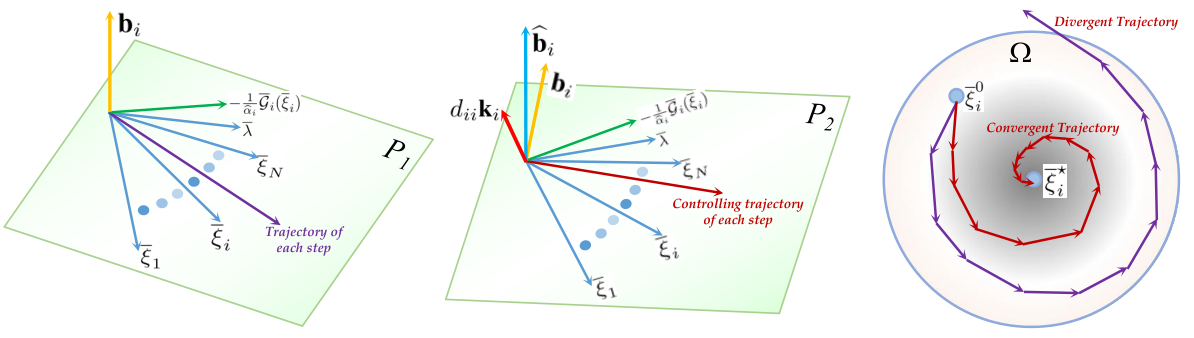
Figure 1: Left: Based on a real space (ξ¯1,⋯,ξ¯N,λ¯)(\overline{\xi}_{1},\cdots,\overline{\xi}_{N},\overline{\lambda}), a purple trajectory of the ii-th variable ξ¯i\overline{\xi}_{i} in each updating step is synthetized by a hyperplane P1P_{1} with the parameter normal vector bi\textbf{b}_{i}. Middle: A scarlet trajectory of the ii-th variable ξ¯i\overline{\xi}_{i} is controlled by a hyperplane P2P_{2} with a new parameter normal vector b^i=bi+ki​i​ki\widehat{\textbf{b}}_{i}=\textbf{b}_{i}+k_{ii}\textbf{k}_{i}. Right: The divergent and convergent trajectories are plotted in the area Ω\Omega.

4.3.2 Controlling PJ-ADMM (2.2)

In this subsection, PJ-ADMM (2.2) can be controlled by the parameter matrix K. In particular, the ii-th row nonzero vector ki=(ki​1,⋯,ki​j,⋯,ki⁡(N+1)){\color[rgb]{0.98,0,0}\textbf{k}_{i}}=({\color[rgb]{0.98,0,0}k_{i1}},{\color[rgb]{0.98,0,0}\cdots},{\color[rgb]{0.98,0,0}k_{ij}},{\color[rgb]{0.98,0,0}\cdots},{\color[rgb]{0.98,0,0}k_{i(N\hskip-1.42271pt+\hskip-1.42271pt1)}}) of K is designed to revise the ii-th updating rule in PJ-ADMM (2.2) as:

{xik+1=arg​minxi​fi​(xi)+β2|(1+ki​i)​Ai​xi+∑j=1,≠iN(1+ki​j)Ajxjk+β−1(1+ki⁡(N+1))λk−q−q^i∥22+12​‖xi−xik‖Si2,λk+1=(1+k(N+1)​(N+1))​λk−γ​β​(∑j=1N(1+k(N+1)​j)​Aj​xjkCLOSEOPEN−q−q^i),\displaystyle\left\{\hskip-5.69046pt\begin{array}[]{l@{}l}\textbf{x}_{i}^{k+1}=&\mbox{arg}\min_{\textbf{x}_{i}}f_{i}(\textbf{x}_{i})+\frac{\beta}{2}\|(1+{\color[rgb]{0.98,0,0}k_{ii}})\textbf{A}_{i}\textbf{x}_{i}\\ &+\sum_{j=1,\neq i}^{N}(1+{\color[rgb]{0.98,0,0}k_{ij}})\textbf{A}_{j}\textbf{x}_{j}^{k}\\ &+\beta^{-1}(1+{\color[rgb]{0.98,0,0}k_{i(N\hskip-1.42271pt+\hskip-1.42271pt1)}})\lambda^{k}-\textbf{q}-{\color[rgb]{0.98,0,0}\widehat{\textbf{q}}_{i}}\|_{2}^{2}\\ &+\frac{1}{2}\|\textbf{x}_{i}-\textbf{x}_{i}^{k}\|_{{\color[rgb]{0.98,0,0}\textbf{S}_{i}}}^{2},\\ \lambda^{k+1}=&(1+{\color[rgb]{0.98,0,0}k_{(N\hskip-1.42271pt+\hskip-1.42271pt1)(N\hskip-1.42271pt+\hskip-1.42271pt1)}})\lambda^{k}\\ &-\gamma\beta(\sum_{j=1}^{N}(1+{\color[rgb]{0.98,0,0}k_{(N\hskip-1.42271pt+\hskip-1.42271pt1)j}})\textbf{A}_{j}\textbf{x}_{j}^{k}\\ &-\textbf{q}-{\color[rgb]{0.98,0,0}\widehat{\textbf{q}}_{i}}),\end{array}\right.

where Si{\color[rgb]{0.98,0,0}\textbf{S}_{i}} and q^i{\color[rgb]{0.98,0,0}\widehat{\textbf{q}}_{i}} are defined in (4.3.1). Similar to the improved GS-ADMM, the improved PJ-ADMM (4.3.2) is constructed by adding the constraint (4.3.1) into the original GS-ADMM (2.2). It is transformed into the switched system (27) with B^=B+DK\widehat{\textbf{B}}=\textbf{B}+\textbf{D}\textbf{K}. Following the Theorem 3, K is established in the following Corollary 2.

Corollary 2. Suppose that Assumption 1 holds. Fixing 0<τ<10<\tau<1, if there exist (N+1)×(N+1)(N\hskip-2.84544pt+\hskip-2.84544pt1)\hskip-2.84544pt\times\hskip-2.84544pt(N\hskip-2.84544pt+\hskip-2.84544pt1) positive definite matrices P=PT≻0\textbf{P}=\textbf{P}^{T}\succ 0, matrices U3,V,H∈ℝ(N+1)×(N+1)\textbf{U}_{3},\textbf{V},\textbf{H}\in\mathbb{R}^{(N\hskip-1.42271pt+\hskip-1.42271pt1)\times(N\hskip-1.42271pt+\hskip-1.42271pt1)} and nonnegative constants Γ=diag​(ι1,⋯,ιN+1)>0\Gamma=\mbox{diag}(\iota_{1},\cdots,\iota_{N\hskip-1.42271pt+\hskip-1.42271pt1})>0 such that the linear matrix inequalities:

(−τ2​P+Γ​F1Γ​F2BT​U3T+HT​DT⋆ΓCT​U3T⋆⋆P−U3T−U3)<0,\displaystyle\left(\hskip-5.69046pt\begin{array}[]{ccc}-\tau^{2}\textbf{P}+\Gamma\textbf{F}_{1}&\Gamma\textbf{F}_{2}&\textbf{B}^{T}\textbf{U}_{3}^{T}+\textbf{H}^{T}\textbf{D}^{T}\\ \star&\Gamma&\textbf{C}^{T}\textbf{U}_{3}^{T}\\ \star&\star&\textbf{P}-\textbf{U}_{3}^{T}-\textbf{U}_{3}\\ \end{array}\hskip-5.69046pt\right)<0,
a​n​dU3​D=DV,\displaystyle\ \ \ and\ \ \ \ \ \textbf{U}_{3}\textbf{D}=\textbf{D}\textbf{V}, (58)

where F1\textbf{F}_{1} and F2\textbf{F}_{2} are defined in (3), then K=V−1​H\textbf{K}=\textbf{V}^{-1}\textbf{H} drives that PJ-ADMM is linear convergent.

Corollary 2 builds the parameter controller K to obtain the linear convergence of divergent PJ-ADMM by stabilizing the system (27). In fact, the the trajectory of each variable is adjusted by the corresponding row vector of K. Following the linear transformation in Remark 5, the control theories are proposed in Section S7 in supplementary materials.

Discussion: The convergence of two-block ADMM (Nishihara et al., 2015) and some gradient methods (i.e. the Heavy-ball method and Nesterov’s accelerated method) (Lessard et al., 2016; Hu & Lessard, 2017) were proved by using the integral quadratic constraint (IQC) (Megretski & Rantzer, 1997). In addition, IQC was also used to analyze the stochastic optimization methods (Hu et al., 2017), and an optimized network (OptNet) architecture was presented to integrate differentiable optimization problems (specifically, in the form of quadratic programs) (Amos & Kolter, 2017). However, these methods do not analyze multi-block ADMM algorithms with multi-variable. More importantly, all of them do not consider the parameter control problem in these algorithms. We employ the switched control theory to design and control the multi-block ADMM algorithms.

4.4 A Geometric Interpretation for Controllers

In this subsection, we give a geometric interpretation to better understand the parameter controllers Ki\textbf{K}_{i} for GS-ADMM and K for PJ-ADMM. We first show the geometric shapes of GS-ADMM and PJ-ADMM. Following the Propositions 1, 2 and the transformations in the subsection 3, GS-ADMM (2.2) and PJ-ADMM (2.2) are transformed into the system (25) with B^i=Bi\widehat{\textbf{B}}_{i}=\textbf{B}_{i} and the system (27) with B^=B\widehat{\textbf{B}}=\textbf{B}, respectively. Considering one block variable ξ¯i=ξi−ξi⋆\overline{\xi}_{i}=\xi_{i}-\xi_{i}^{\star}, where ξi=Ai​xi\xi_{i}=\textbf{A}_{i}\textbf{x}_{i} and ξi⋆=Ai​xi⋆\xi_{i}^{\star}=\textbf{A}_{i}\textbf{x}_{i}^{\star}, their updating rules are converted into the recursive forms:

ξ¯ik+1=−∑j<iβα^iξ¯jk+1+(1−βα^i)ξ¯ik−∑j>iNβα^iξ¯jk−1α^iλ¯k−1α^i𝒢¯i(ξ¯ik),\displaystyle\begin{array}[]{l@{}l}\overline{\xi}_{i}^{k+1}=&-\sum_{j<i}\frac{\beta}{\widehat{\alpha}_{i}}\overline{\xi}_{j}^{k+1}+(1-\frac{\beta}{\widehat{\alpha}_{i}})\overline{\xi}_{i}^{k}\\ &-\sum_{j>i}^{N}\frac{\beta}{\widehat{\alpha}_{i}}\overline{\xi}_{j}^{k}-\frac{1}{\widehat{\alpha}_{i}}\overline{\lambda}^{k}-\frac{1}{\widehat{\alpha}_{i}}\overline{\mathcal{G}}_{i}(\overline{\xi}_{i}^{k}),\end{array}
ξ¯ik+1=−1α^i​λ¯k+(1−βα^i)​ξ¯ik−∑j=1,≠iNβα^i​ξ¯jk−1α^i​𝒢¯i​(ξ¯ik).\displaystyle\begin{array}[]{l@{}l}\overline{\xi}_{i}^{k+1}=&-\frac{1}{\widehat{\alpha}_{i}}\overline{\lambda}^{k}+(1-\frac{\beta}{\widehat{\alpha}_{i}})\overline{\xi}_{i}^{k}-\sum_{j=1,\neq i}^{N}\frac{\beta}{\widehat{\alpha}_{i}}\overline{\xi}_{j}^{k}\\ &-\frac{1}{\widehat{\alpha}_{i}}\overline{\mathcal{G}}_{i}(\overline{\xi}_{i}^{k}).\end{array}

Following in a real space (ξ¯1,⋯,ξ¯N,λ¯)(\overline{\xi}_{1},\cdots,\overline{\xi}_{N},\overline{\lambda}), the trajectory of the variable ξ¯i\overline{\xi}_{i} is based on a gradient term −1α^i​𝒢¯i​(ξ¯i)-\frac{1}{\widehat{\alpha}_{i}}\overline{\mathcal{G}}_{i}(\overline{\xi}_{i}) and a hyperplane P1P_{1} pattern with a normal (or parameter) vector bi=[−βα^1,⋯,−βα^i−1,1−βα^i,−βα^i+1,⋯,\textbf{b}_{i}=[-\frac{\beta}{\widehat{\alpha}_{1}},\cdots,-\frac{\beta}{\widehat{\alpha}_{i-1}},1-\frac{\beta}{\widehat{\alpha}_{i}},-\frac{\beta}{\widehat{\alpha}_{i+1}},\cdots, −βα^i,−1α^i]-\frac{\beta}{\widehat{\alpha}_{i}},-\frac{1}{\widehat{\alpha}_{i}}] in the left of Fig. 1. Given an initial point ξ¯0\overline{\xi}^{0}, since the purple trajectory ξ¯it+1\overline{\xi}_{i}^{t+1} is computed by (4.4) or (4.4), its direction is determined by the parameter vector bi\textbf{b}_{i}, which corresponds to the ii-th row vector of the parameter matrices Bi\textbf{B}_{i} or B.

When this purple trajectory is divergent in the right of Fig. 1, it is desired to find a suitable normal vector to make ξ¯it+1\overline{\xi}_{i}^{t+1} convergent. Our parameter controllers Ki\textbf{K}_{i} and K are used to control GS-ADMM and PJ-ADMM. Their improved versions are shown in (4.3.1) and (4.3.2), which are converted into the system (25) with B^i=Bi+Di​Ki\widehat{\textbf{B}}_{i}=\textbf{B}_{i}+\textbf{D}_{i}\textbf{K}_{i} and the system (27) with B^=B+DK\widehat{\textbf{B}}=\textbf{B}+\textbf{D}\textbf{K}, respectively. Similar to (4.4) and (4.4), the new rules of ξ¯i\overline{\xi}_{i} are changed into the recursive forms:

ξ¯ik+1=−∑j<iβα^i(1+ki​j)ξ¯jk+1+(1−βα^i​(1+ki​i))​ξ¯ik−∑j>iNβα^i​(1+ki​j)​ξ¯jk−1α^i​(1+ki⁡(N+1))​λ¯k−1α^i​𝒢¯i​(ξ¯ik),\displaystyle\begin{array}[]{l@{}l}\overline{\xi}_{i}^{k+1}=&-\sum_{j<i}\frac{\beta}{\widehat{\alpha}_{i}}(1+{\color[rgb]{0.98,0,0}k_{ij}})\overline{\xi}_{j}^{k+1}\\ &+(1-\frac{\beta}{\widehat{\alpha}_{i}}(1+{\color[rgb]{0.98,0,0}k_{ii}}))\overline{\xi}_{i}^{k}-\sum_{j>i}^{N}\frac{\beta}{\widehat{\alpha}_{i}}(1+{\color[rgb]{0.98,0,0}k_{ij}})\overline{\xi}_{j}^{k}\\ &-\frac{1}{\widehat{\alpha}_{i}}(1+{\color[rgb]{0.98,0,0}k_{i(N\hskip-1.42271pt+\hskip-1.42271pt1)}})\overline{\lambda}^{k}-\frac{1}{\widehat{\alpha}_{i}}\overline{\mathcal{G}}_{i}(\overline{\xi}_{i}^{k}),\end{array}
ξ¯ik+1=−∑j=1,≠iNβα^i(1+ki​j)ξ¯jk+(1−βα^i​(1+ki​j))​ξ¯ik−1α^i​(1+ki⁡(N+1))​λ¯k−1α^i​𝒢¯i​(ξ¯ik).\displaystyle\begin{array}[]{l@{}l}\overline{\xi}_{i}^{k+1}=&-\sum_{j=1,\neq i}^{N}\frac{\beta}{\widehat{\alpha}_{i}}(1+{\color[rgb]{0.98,0,0}k_{ij}})\overline{\xi}_{j}^{k}\\ &+(1-\frac{\beta}{\widehat{\alpha}_{i}}(1+{\color[rgb]{0.98,0,0}k_{ij}}))\overline{\xi}_{i}^{k}\\ &-\frac{1}{\widehat{\alpha}_{i}}(1+{\color[rgb]{0.98,0,0}k_{i(N\hskip-1.42271pt+\hskip-1.42271pt1)}})\overline{\lambda}^{k}-\frac{1}{\widehat{\alpha}_{i}}\overline{\mathcal{G}}_{i}(\overline{\xi}_{i}^{k}).\end{array}

The vector ki\textbf{k}_{i} is designed to update bi\textbf{b}_{i} as a new parameter vector b^i\widehat{\textbf{b}}_{i} for the hyperplane P2P_{2} pattern in the middle of Fig. 1, where b^i=bi+di​i​ki\widehat{\textbf{b}}_{i}=\textbf{b}_{i}+d_{ii}\textbf{k}_{i} and di​i=−βα^id_{ii}=-\frac{\beta}{\widehat{\alpha}_{i}}. Thus, the direction of the trajectory ξ¯it+1\overline{\xi}_{i}^{t+1} is intuitively improved by the vector b^i\widehat{\textbf{b}}_{i}. For example, the purple trajectory is revised as the scarlet trajectory in the right of Fig. 1.

Why the parameter controllers ω⁡(ξ¯)=DK​ξ¯\omega(\overline{\xi})=\textbf{D}\textbf{K}\overline{\xi} does not change the equilibrium point ξ¯⋆=0\overline{\xi}^{\star}=0 of PJ-ADMM? First, the system (27) with B^=B\widehat{\textbf{B}}=\textbf{B} has the unique equilibrium point ξ¯⋆=0\overline{\xi}^{\star}=0 since the problem (1) is convex. Second, ξ¯⋆=0\overline{\xi}^{\star}=0 is an equilibrium point of the system (27) with B^=B+DK\widehat{\textbf{B}}=\textbf{B}+\textbf{D}\textbf{K} because of ω⁡(ξ¯⋆)=DK​ξ¯⋆=0\omega(\overline{\xi}^{\star})=\textbf{D}\textbf{K}\overline{\xi}^{\star}=0. Third, the corresponding optimization problem is still convex because the feedback controller is a linear equality constraint. Thus, the equilibrium point ξ¯⋆=0\overline{\xi}^{\star}=0 is unique for the system (27) with B^=B+DK\widehat{\textbf{B}}=\textbf{B}+\textbf{D}\textbf{K}. In fact, the key idea is to let the action of the ADMMs at any moment in time depend on the actual behavior of the the ADMMs that is being controlled. This idea imposes a certain ’smart’ controller, which decides on the direction of the variables in the next moment. Similarly, ω⁡(ξ¯i)=Di​Ki​ξ¯i\omega(\overline{\xi}_{i})=\textbf{D}_{i}\textbf{K}_{i}\overline{\xi}_{i} does not change the equilibrium point ξ¯i⋆=0\overline{\xi}_{i}^{\star}=0 of GS-ADMM.

An example. Here we consider the following strongly convex problem with three variables (Chen et al., 2016):

minx1,x2,x3\displaystyle\min_{x_{1},x_{2},x_{3}}\ 0.05​x12+0.05​x22+0.05​x32,\displaystyle 0.05x_{1}^{2}+0.05x_{2}^{2}+0.05x_{3}^{2}, (69)
​s.t.\displaystyle\emph{s.t.}\ A1​x1+A2​x2+A3​x3=0,\displaystyle\textbf{A}_{1}x_{1}+\textbf{A}_{2}x_{2}+\textbf{A}_{3}x_{3}=\textbf{0},

where A1=[1,1,1]T\textbf{A}_{1}=[1,1,1]^{T}, A2=[1,1,2]T\textbf{A}_{2}=[1,1,2]^{T} and A3=[1,2,2]T\textbf{A}_{3}=[1,2,2]^{T}. The unique equilibrium point is x1=x2=x3=0x_{1}=x_{2}=x_{3}=0. By employing the PJ-ADMM with the parameters β=1\beta=1, γ=1\gamma=1, and Lagrange multipliers λ=[λ1,λ2,λ3]T\lambda=[\lambda_{1},\lambda_{2},\lambda_{3}]^{T} to solve this problem (69), it is divergent (Chen et al., 2016). Based on our Proposition 2, the problem (69) is transformed into a the dynamical system (27) with the state ξ¯=(x1,x2,x3,λ1,λ2,λ3)T\overline{\xi}=(x_{1},x_{2},x_{3},\lambda_{1},\lambda_{2},\lambda_{3})^{T}. By employing the condition in Corollary C6 (in Section S7) or Corollary 2 with β=1\beta=1, γ=1\gamma=1, α=1\alpha=1 and τ=0.9\tau=0.9, we design a parameter matrix K to control the divergent ADMM, where 𝐊=[−0.65000.04000.01000.1000−0.2000−0.00000.0400−0.72000.0200−0.0000−0.20000.20000.01000.0200−0.88000.1000−0.00000.10000.1000−0.00000.1000−1.00000.00000.0000−0.2000−0.20000.00000.0000−1.00000.0000−0.00000.20000.1000−0.0000−0.0000−1.0000].\mathbf{K}=\begin{bmatrix}[r]-0.6500&0.0400&0.0100&0.1000&-0.2000&-0.0000\\ 0.0400&-0.7200&0.0200&-0.0000&-0.2000&0.2000\\ 0.0100&0.0200&-0.8800&0.1000&-0.0000&0.1000\\ 0.1000&-0.0000&0.1000&-1.0000&0.0000&0.0000\\ -0.2000&-0.2000&0.0000&0.0000&-1.0000&0.0000\\ -0.0000&0.2000&0.1000&-0.0000&-0.0000&-1.0000\\ \end{bmatrix}. Each row vector of K is used to construct a linear equality constraint for the corresponding variable. For instance, k1=(−0.65,0.04,0.01,0.10,−0.20,0.00)\textbf{k}_{1}=(-0.65,0.04,0.01,0.10,-0.20,0.00) creates a constraint (hyperplane) −0.65​x1+0.04​x2+0.01​x3+0.10​λ1+0.20​λ2+0​λ3=0-0.65x_{1}+0.04x_{2}+0.01x_{3}+0.10\lambda_{1}+0.20\lambda_{2}+0\lambda_{3}=0 for x1x_{1}. The normal vector k1\textbf{k}_{1} to adjust the direction of the trajectory of x1x_{1}. Similar to (4.3.2), the controller ω⁡(ξ¯)=K​ξ¯\omega(\overline{\xi})=\textbf{K}\overline{\xi} is added into the the divergent ADMM to make it convergent for solving the problem (69).

Note that all proofs of our theories and more numerical experiments are respectively provided in Sections S8 and S9 in supplementary materials.

5 Conclusion

In this paper, we developed a switched Lyapunov framework to study the three basic problems of multi-block ADMM: building the convergence under arbitrary or given switching sequences, finding convergent switching sequences, and designing the fixed parameters. First, we employed switched quadratic Lyapunov functions to provide sufficient conditions to guarantee that multi-block ADMM is convergent. Second, based on the sufficient conditions, we proposed a backtracking algorithm to search for the convergent switching sequences. Third, we designed parameter controllers to make multi-block ADMM convergent. These controllers were in essence equality constraints to reduce the complexity of the original multi-block ADMM. Finally, a geometric interpretation showed the parameter controllers adjusted directions of trajectories of the variables. More importantly, this paper provided a new direction to analyze the multi-block ADMM by employing the switched control theory.

References

  • Amos & Kolter (2017) Amos, B. and Kolter, J. Z. Optnet: Differentiable optimization as a layer in neural networks. In Precup, D. and Teh, Y. W. (eds.), Proceedings of the International Conference on Machine Learning, pp. 136–145, Sydney, Australia, 2017.
  • Boyd et al. (1994) Boyd, S., Ghaoui, L.E., Feron, E., and Balakrishnan., V. Linear Matrix Inequalities in System and Control Theory. SIAM, 1994.
  • Boyd et al. (2011) Boyd, S., Parikh, N., Chu, E., Peleato, B., and Eckstein, J. Distributed optimization and statistical learning via the alternating direction method of multipliers. Foundations and Trends in Machine Learning, 3(1):1–122, 2011.
  • Chang et al. (2016) Chang, T. H., Hong, M. Y., Liao, W.C., and Wang, X. F. Asynchronous distributed admm for large-scale optimization-part i: Algorithm and convergence analysis. IEEE Transactions on Signal Processing, 64(12):3118–3130, 2016.
  • Chen et al. (2016) Chen, C.H., He, B.S., Ye, Y.Y., and Yuan, X.M. The direct extension of admm for multi-block convex minimization problems is not necessarily convergent. Mathematical Programming, Ser. A, 155(1):57–79, 2016.
  • Daafouz et al. (2002) Daafouz, J., Riedinger, P., and Iung, C. Stability analysis and control synthesis for switched systems: A switched lyapunov function approach. IEEE Transactions on Automatic Control, 47(12):1883–1887, 2002.
  • Deng & Yin (2016) Deng, W. and Yin, W. T. On the global and linear convergence of the generalized alternating direction method of multipliers. Journal of Scientific Computing, 66(3):889–916, 2016.
  • Deng et al. (2017) Deng, W., Lai, M. J., Peng, Z. M., and Yin, W. T. Parallel multi-block admm with 𝒪⁡(1/k)\mathcal{O}(1/k) convergence. Journal of Scientific Computing, 71(2):712–736, 2017.
  • Eckstein & Bertsekas (1992) Eckstein, J. and Bertsekas, D.P. On the douglas-rachford splitting method and the proximal point algorithm for maximal monotone operators. Mathematical Programming, 55(1):293–318, 1992.
  • Fang et al. (2004) Fang, L., Lin, H., and Antsaklis, P. J. Stabilization and performance analysis for a class of switched systems. In Proceedings of the IEEE Conference on Decision and Control, pp. 3265–3270, Atlantis, Paradise Island, Bahamas, 2004.
  • Gabay & Mercier (1976) Gabay, D. and Mercier, B. A dual algorithm for the solution of nonlinear variational problems via finite element approximation. Computers &\& Mathematics with Applications, 2(1):17–40, 1976.
  • Glowinski & Marrocco (1975) Glowinski, R. and Marrocco, A. Sur l’approximation, par éléents finis d’ordre un, et la réolution, par péalisation-dualité d’une classe de problèmes de dirichlet non linéires. ESAIM Mathematical Modelling and Numerical Analysis, 9(R2):41–76, 1975.
  • Han & Yuan (2012) Han, D.R. and Yuan, X.M. A note on the alternating direction method of multipliers. Journal of Optimization Theory and Applications, 155(1):227–238, 2012.
  • Hong et al. (2016) Hong, M. Y., Razaviyayn, M., Luo, Z. Q., and Pang, J. S. A unified algorithmic framework for block-structured optimization involving big data. IEEE Signal Processing Magazine, 33(1):57–77, 2016.
  • Hu & Lessard (2017) Hu, B. and Lessard, L. Dissipativity theory for nesterov’s accelerated method. In Precup, D. and Teh, Y. W. (eds.), Proceedings of the International Conference on Machine Learning, pp. 1549–1557, Sydney, Australia, 2017.
  • Hu et al. (2017) Hu, B., Seiler, P., and Rantzer, A. A unified analysis of stochastic optimization methods using jump system theory and quadratic constraints. In Kale, S. and Shamir, O. (eds.), Proceedings of the International Conference on Learning Theory, pp. 1157–1189, Amsterdam, Netherlands, 2017.
  • Lessard et al. (2016) Lessard, L., Recht, B., and Packard, A. Analysis and design of optimization algorithms via integral quadratic constraints. SIAM Journal on Optimization, 26(1):57–95, 2016.
  • Li et al. (2016) Li, X.D., Sun, D.F., and Toh, K.C. A schur complement based semi-proximal admm for convex quadratic conic programming and extensions. Mathematical Programming, Ser. A, 155(1):333–373, 2016.
  • Liberzon et al. (1999) Liberzon, Daniel, Hespanha, João Pedro, and Morse, A. Stephen. Stability of switched linear systems: a Lie-algebraic condition. Syst. and Contr. Lett., 37(3):117–122, June 1999.
  • Lin & Antsaklis (2009) Lin, H. and Antsaklis, P. J. Stability and stabilizability of switched linear systems: A survey of recent results. IEEE Transactions on Automatic Control, 54(2):308–322, 2009.
  • Lin et al. (2015a) Lin, T.Y., Ma, S.Q., and Zhang, S.Z. On the global linear convergence of the admm with multi-block variables. SIAM Journal on Optimization, 25(3):1478–1497, 2015a.
  • Lin et al. (2015b) Lin, T.Y., Ma, S.Q., and Zhang, S.Z. On the sublinear convergence rate of multi-block admm. Journal of the Operations Research Society of China, 3(3):251–274, 2015b.
  • Lin et al. (2016) Lin, T.Y., Ma, S.Q., and Zhang, S.Z. Iteration complexity analysis of multi-block admm for a family of convex minimization without strong convexity. Journal of Scientific Computing, 69(1):52–81, 2016.
  • Lu et al. (2016) Lu, C.Y., Li, H., Lin, Z.C., and Yan, S.C. Fast proximal linearized alternating direction method of multiplier with parallel splitting. In Proceedings of the Thirty AAAI Conference on Artificial Intelligence, pp. 739–745, Phoenix, Arizona USA, 2016.
  • Lu et al. (2017) Lu, C.Y., Feng, J.S., Yan, S.C., and Lin, Z.C. A unified alternating direction method of multipliers by majorization minimization. IEEE Transactions on Pattern Analysis and Machine Intelligence, 2017.
  • Mason & Shorten (2004) Mason, O. and Shorten, R. On common quadratic lyapunov functions for stable discrete-time lti systems. IMA Journal of Applied Mathematics, 69:271–283, 2004.
  • Megretski & Rantzer (1997) Megretski, A. and Rantzer, A. System analysis via integral quadratic constraints. IEEE Trans. Automat. Control, 42(6):819–830, 1997.
  • Nishihara et al. (2015) Nishihara, R., Lessard, L., Recht, B., Packard, A., and Jordan, M. I. A general analysis of the convergence of admm. In Bach, F. and Blei, D. (eds.), Proceedings of the International Conference on Machine Learning, pp. 343–352, Lille, France, 2015.
  • Parikh & Boyd (2014) Parikh, N. and Boyd, S. Proximal algorithms. Foundations and Trends in Optimization, 1(3):127–239, 2014.
  • Sun et al. (2015) Sun, D.F., Toh, K.C., and Yang, L.Q. A convergent 3-block semiproximal alternating direction method of multipliers for conic programming with 4-type constraints. SIAM Journal on Optimization, 25(2):882–915, 2015.
  • Wang et al. (2017) Wang, J. L., Kolar, M., Srebro, N., and Zhang, T. Efficient distributed learning with sparsity. In Precup, D. and Teh, Y. W. (eds.), Proceedings of the International Conference on Machine Learning, pp. 3636–3645, Sydney, Australia, 2017.
  • Wu et al. (2010) Wu, M., He, Y., and She, J. H. Stability Analysis and Robust Control of Time-Delay Systems. Science Press Beijing and Springer-Verlag Berlin Heidelberg, 1nd edition, 2010.
  • Xu et al. (2017) Xu, Y., Liu, M.R., Q.H. Lin, Qihang, and Yang, T.B. Admm without a fixed penalty parameter: Faster convergence with new adaptive penalization. In Proceedings of the Advances in Neural Information Processing Systems, pp. 1267–1277, 2017.

Classical ADMMs

Classical ADMMs can be categorized into Gauss-Seidel ADMM and Jacobian ADMM. The iterative scheme of the Gauss-Seidel ADMM (GS-ADMM) is outlined below: for 1≤i≤N1\leq i\leq N,

{xik+1=arg​minxi​fi​(xi)+β2​‖∑j<iAj​xjk+1+Ai​xi+∑j>iAj​xjk+β−1​λk−q‖22+12​‖xi−xik‖Si2,λk+1=λk−γ​β​(∑j=1NAj​xjk+1−q),\displaystyle\left\{\hskip-5.69046pt\begin{array}[]{l@{}l}\textbf{x}_{i}^{k+1}=&\mbox{arg}\min_{\textbf{x}_{i}}f_{i}(\textbf{x}_{i})+\frac{\beta}{2}\|\sum_{j<i}\textbf{A}_{j}\textbf{x}_{j}^{k+1}+\textbf{A}_{i}\textbf{x}_{i}+\sum_{j>i}\textbf{A}_{j}\textbf{x}_{j}^{k}+\beta^{-1}\lambda^{k}-\textbf{q}\|_{2}^{2}+\frac{1}{2}\|\textbf{x}_{i}-\textbf{x}_{i}^{k}\|_{\textbf{S}_{i}}^{2},\\ \lambda^{k+1}=&\lambda^{k}-\gamma\beta(\sum_{j=1}^{N}\textbf{A}_{j}\textbf{x}_{j}^{k+1}-\textbf{q}),\end{array}\right.

A general Jacobian ADMM, Proximal-Jacobian ADMM (PJ-ADMM), updates the variable xi\textbf{x}_{i} in parallel by: for 1≤i≤N1\leq i\leq N,

{xik+1=arg​minxi​fi​(xi)+β2​‖∑j=1,≠iNAj​xjk+Ai​xi+β−1​λk−q‖22+12​‖xi−xik‖Si2,λk+1=λk−γ​β​(∑j=1NAj​xjk−q),\displaystyle\left\{\hskip-5.69046pt\begin{array}[]{l@{}l}\textbf{x}_{i}^{k+1}=&\mbox{arg}\min_{\textbf{x}_{i}}f_{i}(\textbf{x}_{i})+\frac{\beta}{2}\|\sum_{j=1,\neq i}^{N}\textbf{A}_{j}\textbf{x}_{j}^{k}+\textbf{A}_{i}\textbf{x}_{i}+\beta^{-1}\lambda^{k}-\textbf{q}\|_{2}^{2}+\frac{1}{2}\|\textbf{x}_{i}-\textbf{x}_{i}^{k}\|_{\textbf{S}_{i}}^{2},\\ \lambda^{k+1}=&\lambda^{k}-\gamma\beta(\sum_{j=1}^{N}\textbf{A}_{j}\textbf{x}_{j}^{k}-\textbf{q}),\end{array}\right.

where ‖xi‖Si2=xiT​Si​xi\|\textbf{x}_{i}\|_{\textbf{S}_{i}}^{2}=\textbf{x}_{i}^{T}\textbf{S}_{i}\textbf{x}_{i}, Si=αi​I−β​AiT​Ai\textbf{S}_{i}=\alpha_{i}\textbf{I}-\beta\textbf{A}_{i}^{T}\textbf{A}_{i} (αi>0)(\alpha_{i}>0) and γ>0\gamma>0 is a damping parameter.

S6 Building Convergence Conditions for Challenge 1 with Linear Transformation

We consider a linear transformation of the switched systems. When the gradient of nonlinear functions 𝔤i​(x)\mathfrak{g}_{i}(x) can be (approximately) linearized as 𝔤i​(x)=gi​x\mathfrak{g}_{i}(x)=\mathrm{g}_{i}x (1≤i≤N)(1\leq i\leq N), where gi\mathrm{g}_{i} is a linearized parameter. For example, fif_{i} is a quadratic function, or the popular proximal function Proxθ​𝔤​(x)=arg​miny​{θ​𝔤​(x)−‖x−y‖2}\textbf{Prox}_{\theta}\mathfrak{g}(x)=\hbox{arg}\min_{y}\{\theta\mathfrak{g}(x)-||x-y||^{2}\} can be transformed as the following form Proxθ​𝔤​(x)=g​x\textbf{Prox}_{\theta}\mathfrak{g}(x)=\mathrm{g}x, where g={|x|−θ|x|,if |x|>θ,0,otherwise.\mathrm{g}=\left\{\begin{array}[]{ll}\frac{|x|-\theta}{|x|},&\hbox{if $|x|>\theta$,}\\ 0,&\hbox{otherwise.}\end{array}\right.. The nonlinear function 𝒢⁡(ξ)\mathcal{G}(\xi) in Eq. (20) in the main body is linearized as 𝒢⁡(ξ)=(Gi⊗Id)​ξ¯\mathcal{G}(\xi)=(\textbf{G}_{i}\otimes\textbf{I}_{d})\overline{\xi}, where Gi=𝕀N+1i​G\textbf{G}_{i}=\mathbb{I}_{N+1}^{i}\textbf{G} and G=diag(g1,⋯gN,0)\textbf{G}=\hbox{diag}\left(\mathrm{g}_{1},\cdots\mathrm{g}_{N},0\right). Thus,

S6.1 linearized GS-ADMM

The switched system in Eq. (25) in the main body for GS-ADMM is rewritten as a following linear switched system:

ξ¯t+1=(B¯i⊗Id)​ξ¯t,i∈ℐ,\displaystyle\overline{\xi}^{t+1}=(\overline{\textbf{B}}_{i}\otimes\textbf{I}_{d})\overline{\xi}^{t},\ \ i\in\mathcal{I}, (S74)

where B¯i=B^i+Ci​Gi\overline{\textbf{B}}_{i}=\widehat{\textbf{B}}_{i}+\textbf{C}_{i}\textbf{G}_{i}. Based on the Corollary 1, Theorems 1 and 2 in the main body, we have the following Corollary C1.

Corollary C1. Suppose that Assumption 1 holds. Fixing 0<τ<10<\tau<1, the linearized GS-ADMM under arbitrary sequence is linear convergent, if there exist (N+1)×(N+1)(N\hskip-2.84544pt+\hskip-2.84544pt1)\hskip-2.84544pt\times\hskip-2.84544pt(N\hskip-2.84544pt+\hskip-2.84544pt1) positive definite matrices P=PT>0\textbf{P}=\textbf{P}^{T}>0, Pi=PiT>0\textbf{P}_{i}=\textbf{P}_{i}^{T}>0, and matrices U1​i,U3​i∈ℝ(N+1)×(N+1)\textbf{U}_{1i},\textbf{U}_{3i}\in\mathbb{R}^{(N\hskip-1.42271pt+\hskip-1.42271pt1)\times(N\hskip-1.42271pt+\hskip-1.42271pt1)} (i∈ℐ)(i\in\mathcal{I}) such that the linear matrix inequalities:∀(i,j)∈ℐ×ℐ\forall(i,j)\in\mathcal{I}\times\mathcal{I},

(U1​i​B¯i+B¯iT​U1​iT−τ2​PiB¯iT​U3​iT−U1​i⋆Pj−U3​iT−U3​i)<0,\displaystyle\left(\hskip-5.69046pt\begin{array}[]{cc}\textbf{U}_{1i}\overline{\textbf{B}}_{i}+\overline{\textbf{B}}_{i}^{T}\textbf{U}_{1i}^{T}-\tau^{2}\textbf{P}_{i}&\overline{\textbf{B}}_{i}^{T}\textbf{U}_{3i}^{T}-\textbf{U}_{1i}\\ \star&\textbf{P}_{j}-\textbf{U}_{3i}^{T}-\textbf{U}_{3i}\\ \end{array}\hskip-5.69046pt\right)<0,

or ∀(i,j)∈ℐ×ℐ\forall(i,j)\in\mathcal{I}\times\mathcal{I},

B¯iT​Pj​B¯i−τ2​Pi<0,\displaystyle\overline{\textbf{B}}_{i}^{T}\textbf{P}_{j}\overline{\textbf{B}}_{i}-\tau^{2}\textbf{P}_{i}<0, (S77)

or ∀i∈ℐ\forall i\in\mathcal{I},

B¯iT​P​B¯i−τ2​P<0.\displaystyle\overline{\textbf{B}}_{i}^{T}\textbf{P}\overline{\textbf{B}}_{i}-\tau^{2}\textbf{P}<0. (S78)

Two conditions in Corollary C1 are provided for the linear convergence of the linearized GS-ADMM as it is used to solve the convex problem in Eq. (1) in the main body with the linearized gradients of the functions, such as Quadratic Programming problems.

S6.2 linearized PJ-ADMM

Similar to the linearized GS-ADMM, the system in Eq. (27) for PJ-ADMM in the main body is rewritten as a following linear system:

ξ¯t+1=(B¯⊗Id)​ξ¯t,\displaystyle\overline{\xi}^{t+1}=(\overline{\textbf{B}}\otimes\textbf{I}_{d})\overline{\xi}^{t}, (S79)

where B¯=B^+CG\overline{\textbf{B}}=\widehat{\textbf{B}}+\textbf{C}\textbf{G}. Based on the Corollary C1, we have the following corollary C2.

Corollary C2. Suppose that Assumption 1 holds. Fixing 0<τ<10<\tau<1, the linearized PJ-ADMM is linear convergent, if there exist (N+1)×(N+1)(N\hskip-2.84544pt+\hskip-2.84544pt1)\hskip-2.84544pt\times\hskip-2.84544pt(N\hskip-2.84544pt+\hskip-2.84544pt1) positive definite matrices P=PT>0\textbf{P}=\textbf{P}^{T}>0, and matrices U1,U3∈ℝ(N+1)×(N+1)\textbf{U}_{1},\textbf{U}_{3}\in\mathbb{R}^{(N\hskip-1.42271pt+\hskip-1.42271pt1)\times(N\hskip-1.42271pt+\hskip-1.42271pt1)} such that the linear matrix inequalities:

(U1​B¯+B¯T​U1T−τ2​PB¯T​U3T−U1⋆P−U3T−U3)<0,\displaystyle\left(\hskip-5.69046pt\begin{array}[]{cc}\textbf{U}_{1}\overline{\textbf{B}}+\overline{\textbf{B}}^{T}\textbf{U}_{1}^{T}-\tau^{2}\textbf{P}&\overline{\textbf{B}}^{T}\textbf{U}_{3}^{T}-\textbf{U}_{1}\\ \star&\textbf{P}-\textbf{U}_{3}^{T}-\textbf{U}_{3}\\ \end{array}\hskip-5.69046pt\right)<0,

or

B¯T​P​B¯−τ2​P<0.\displaystyle\overline{\textbf{B}}^{T}\textbf{P}\overline{\textbf{B}}-\tau^{2}\textbf{P}<0. (S82)

S7 Designing Parameter Controllers for Challenge 3 with Linear Transformation

Following the linear transformation in the above section, in this subsection we can control the parameters by designing controllers to stabilize the linear switched control systems for the convergence of ADMMs with linear transformation.

S7.1 Controlling GS-ADMM (S83) with Linear Transformation

The switched system in Eq. (25) in the main body is rewritten as the following linear switched control system:

ξ¯t+1=((B¯i+Di​Ki)⊗Id)​ξ¯t,i∈ℐ,\displaystyle\overline{\xi}^{t+1}=((\overline{\textbf{B}}_{i}+\textbf{D}_{i}\textbf{K}_{i})\otimes\textbf{I}_{d})\overline{\xi}^{t},\ \ i\in\mathcal{I}, (S83)

where B¯i=Bi+Ci​Gi\overline{\textbf{B}}_{i}=\textbf{B}_{i}+\textbf{C}_{i}\textbf{G}_{i} is defined in (S74).

Based on the conditions (S6.1) in the Corollary C1, it easily obtains the Corollary C3 to design the parameter controllers Ki\textbf{K}_{i} for the linear switched control system (S83).

Corollary C3. Suppose that Assumption 1 holds. Fixing 0<τ<10<\tau<1, if there exist (N+1)×(N+1)(N\hskip-2.84544pt+\hskip-2.84544pt1)\hskip-2.84544pt\times\hskip-2.84544pt(N\hskip-2.84544pt+\hskip-2.84544pt1) positive definite matrices Pi=PiT≻0\textbf{P}_{i}=\textbf{P}_{i}^{T}\succ 0, any matrices U3​i,V=diag​(v1,⋯,vN+1)∈ℝ(N+1)×(N+1)\textbf{U}_{3i},\textbf{V}=\mbox{diag}(v_{1},\cdots,v_{N\hskip-1.42271pt+\hskip-1.42271pt1})\in\mathbb{R}^{(N\hskip-1.42271pt+\hskip-1.42271pt1)\times(N\hskip-1.42271pt+\hskip-1.42271pt1)} (i∈ℐ)(i\in\mathcal{I}) such that the linear matrix inequalities: ∀(i,j)∈ℐ×ℐ\forall(i,j)\in\mathcal{I}\times\mathcal{I},

(−τ2​PiB¯iT​U3​iT+𝕀N+1i​V⋆Pj−U3​iT−U3​i)⪯0,\displaystyle\left(\hskip-5.69046pt\begin{array}[]{ccc}-\tau^{2}\textbf{P}_{i}&\overline{\textbf{B}}_{i}^{T}\textbf{U}_{3i}^{T}+\mathbb{I}_{N+1}^{i}\textbf{V}\\ \star&\textbf{P}_{j}-\textbf{U}_{3i}^{T}-\textbf{U}_{3i}\\ \end{array}\hskip-5.69046pt\right)\preceq 0,

then Ki=vidi​(U3​i−1​𝕀N+1i)T​(i∈ℐ)\textbf{K}_{i}=\frac{v_{i}}{d_{i}}(\textbf{U}_{3i}^{-1}\mathbb{I}_{N+1}^{i})^{T}\ (i\in\mathcal{I}) drive that the linearized GS-ADMM under arbitrary sequence is linear convergent.

According to the condition (S77) in Corollary C1, it is difficult to solve the Ki\textbf{K}_{i} because one can easily show that the resulting inequalities are not jointly convex on Pj\textbf{P}_{j} and Ki\textbf{K}_{i}. So, we consider the condition (S78) in Corollary C1 by employing the CQLFs (Mason & Shorten, 2004) for the system (S83). Thus, the condition (S78) is written as:

(B¯i+Di​Ki)T​P​(B¯i+Di​Ki)−τ2​P<0,∀i∈ℐ.\displaystyle(\overline{\textbf{B}}_{i}+\textbf{D}_{i}\textbf{K}_{i})^{T}\textbf{P}(\overline{\textbf{B}}_{i}+\textbf{D}_{i}\textbf{K}_{i})-\tau^{2}\textbf{P}<0,\ \ \forall i\in\mathcal{I}.

Generally, the problem of solving numerically the above form for (P,Ki)(\textbf{P},\textbf{K}_{i}) is very difficult since it is nonconvex. In order to make this problem numerically well tractable, a sufficient condition is given in the following corollary by employing the Schur complement (Boyd et al., 1994). Therefore, we have the following Corollary C4.

Corollary C4. Suppose that Assumption 1 holds. Fixing 0<τ<10<\tau<1, if there exist matrices Ni\textbf{N}_{i} (i∈ℐ)(i\in\mathcal{I}) and positive definite matrices Q=QT≻0\textbf{Q}=\textbf{Q}^{T}\succ 0 such that:

(−QB¯i​Q+Di​Ni⋆−τ2​Q)<0,∀i∈ℐ,\displaystyle\left(\hskip-5.69046pt\begin{array}[]{cc}-\textbf{Q}&\overline{\textbf{B}}_{i}\textbf{Q}+\textbf{D}_{i}\textbf{N}_{i}\\ \star&-\tau^{2}\textbf{Q}\\ \end{array}\hskip-5.69046pt\right)<0,\ \ \forall i\in\mathcal{I},

then Ki=Ni​Q−1​(i∈ℐ)\textbf{K}_{i}=\textbf{N}_{i}\textbf{Q}^{-1}\ (i\in\mathcal{I}) drives that the linearized GS-ADMM under arbitrary sequence is linear convergent.

S7.2 Controlling GS-ADMM (S88) with Linear Transformation

The switched system in Eq. ((27) in the main body is rewritten as the following linear switched control system:

ξ¯t+1=((B¯+DK)⊗Id)​ξ¯t,\displaystyle\overline{\xi}^{t+1}=((\overline{\textbf{B}}+\textbf{D}\textbf{K})\otimes\textbf{I}_{d})\overline{\xi}^{t}, (S88)

where B¯=B+CG\overline{\textbf{B}}=\textbf{B}+\textbf{C}\textbf{G} is defined in (S79).

Similar to the controlling GS-ADMM (S83), we have the following Corollary C5 based on the condition (S6.2) in Corollary C2.

Corollary C5. Suppose that Assumption 1 holds. Fixing 0<τ<10<\tau<1, if there exist (N+1)×(N+1)(N\hskip-2.84544pt+\hskip-2.84544pt1)\hskip-2.84544pt\times\hskip-2.84544pt(N\hskip-2.84544pt+\hskip-2.84544pt1) positive definite matrices P=PT≻0\textbf{P}=\textbf{P}^{T}\succ 0, and matrices U,V,H∈ℝ(N+1)×(N+1)\textbf{U},\textbf{V},\textbf{H}\in\mathbb{R}^{(N\hskip-1.42271pt+\hskip-1.42271pt1)\times(N\hskip-1.42271pt+\hskip-1.42271pt1)} such that the linear matrix inequalities:

(−τ2​PB¯T​UT+HT​DT⋆P−UT−U)<0,a​n​dUD=DV,\displaystyle\left(\hskip-5.69046pt\begin{array}[]{ccc}-\tau^{2}\textbf{P}&\overline{\textbf{B}}^{T}\textbf{U}^{T}+\textbf{H}^{T}\textbf{D}^{T}\\ \star&\textbf{P}-\textbf{U}^{T}-\textbf{U}\\ \end{array}\hskip-5.69046pt\right)<0,\ \ \ and\ \ \ \ \ \textbf{U}\textbf{D}=\textbf{D}\textbf{V},

then K=V−1​H\textbf{K}=\textbf{V}^{-1}\textbf{H} drives that the linearized PJ-ADMM is linear convergent.

According to the condition (S82) in Corollary C2, the following Corollary C6 is held by by employing the Schur complement (Boyd et al., 1994).

Corollary C6. Suppose that Assumption 1 holds. Fixing 0<τ<10<\tau<1, if there exist matrices N and positive definite matrices Q=QT≻0\textbf{Q}=\textbf{Q}^{T}\succ 0 such that:

(−QB¯​Q+DN⋆−τ2​Q)<0,∀i∈ℐ,\displaystyle\left(\hskip-5.69046pt\begin{array}[]{cc}-\textbf{Q}&\overline{\textbf{B}}\textbf{Q}+\textbf{D}\textbf{N}\\ \star&-\tau^{2}\textbf{Q}\\ \end{array}\hskip-5.69046pt\right)<0,\ \ \forall i\in\mathcal{I},

then K=NQ−1\textbf{K}=\textbf{N}\textbf{Q}^{-1} drives that the linearized PJ-ADMM is linear convergent.

S8 Proofs

Proof of Proposition 1: It is proved by calculating the gradient or the subgradient of xi\textbf{x}_{i}-subproblem in GS-ADMM and set it to zero. Using the fact that Ai\textbf{A}_{i} has full rank and denoting that ξik=Ai​xik\xi_{i}^{k}=\textbf{A}_{i}\textbf{x}_{i}^{k}, the updating rule for xi\textbf{x}_{i} from GS-ADMM (Classical ADMMs) can be rewritten as follows:

xik+1=\displaystyle\textbf{x}_{i}^{k+1}= Ai−1​arg​minξi​fi​(Ai−1​ξi)+β2​‖∑j<iξjk+1+ξi+∑j>iξjk+β−1​λk−c‖22+αi2​‖xi−xik‖2−β2​‖ξi−ξik‖2.\displaystyle\textbf{A}_{i}^{-1}\mbox{arg}\min_{\xi_{i}}f_{i}(\textbf{A}_{i}^{-1}\xi_{i})+\frac{\beta}{2}\|\sum_{j<i}\xi_{j}^{k+1}+\xi_{i}+\sum_{j>i}\xi_{j}^{k}+\beta^{-1}\lambda^{k}-\textbf{c}\|_{2}^{2}+\frac{\alpha_{i}}{2}\|\textbf{x}_{i}-\textbf{x}_{i}^{k}\|^{2}-\frac{\beta}{2}\|\xi_{i}-\xi_{i}^{k}\|^{2}. (S93)

Since ‖ξi−ξik‖2≤‖Ai‖2​‖xi−xik‖2\|\xi_{i}-\xi_{i}^{k}\|^{2}\leq\|\textbf{A}_{i}\|^{2}\|\textbf{x}_{i}-\textbf{x}_{i}^{k}\|^{2}, multiplying through by Ai\textbf{A}_{i} the problem (S93) is transformed into

ξik+1=\displaystyle\xi_{i}^{k+1}= arg​minξi​gi​(ξi)+β2​‖∑j<iξjk+1+ξi+∑j>iξjk+β−1​λk−c‖22+αi2​‖Ai‖2​‖ξi−ξik‖2−β2​‖ξi−ξik‖2.\displaystyle\mbox{arg}\min_{\xi_{i}}g_{i}(\xi_{i})+\frac{\beta}{2}\|\sum_{j<i}\xi_{j}^{k+1}+\xi_{i}+\sum_{j>i}\xi_{j}^{k}+\beta^{-1}\lambda^{k}-\textbf{c}\|_{2}^{2}+\frac{\alpha_{i}}{2\|\textbf{A}_{i}\|^{2}}\|\xi_{i}-\xi_{i}^{k}\|^{2}-\frac{\beta}{2}\|\xi_{i}-\xi_{i}^{k}\|^{2}. (S94)

Denote α^i=αi‖Ai‖2\widehat{\alpha}_{i}=\frac{\alpha_{i}}{\|\textbf{A}_{i}\|^{2}}. The problem (S94) implies that

ξik+1=\displaystyle\xi_{i}^{k+1}= ξik−βα^i​(∑j<iξjk+1+∑j≥iξjk)−1α^i​λk−1α^i​𝔤i​(ξik+1)+βα^i​c,\displaystyle\xi_{i}^{k}-\frac{\beta}{\widehat{\alpha}_{i}}(\sum_{j<i}\xi_{j}^{k+1}+\sum_{j\geq i}\xi_{j}^{k})-\frac{1}{\widehat{\alpha}_{i}}\lambda^{k}-\frac{1}{\widehat{\alpha}_{i}}\mathfrak{g}_{i}(\xi_{i}^{k+1})+\frac{\beta}{\widehat{\alpha}_{i}}\textbf{c},

where 𝔤i​(⋅)\mathfrak{g}_{i}(\cdot) is defined in Eq. (10) in main body, and since 𝔤i​(xik+1)\mathfrak{g}_{i}(\textbf{x}_{i}^{k+1}) is difficult to be directly calculated, it is approximated by 𝔤i​(xik)\mathfrak{g}_{i}(\textbf{x}_{i}^{k}), and we have,

ξik+1=\displaystyle\xi_{i}^{k+1}= ξik−βα^i​(∑j<iξjk+1+∑j≥iξjk)−1α^i​λk−1α^i​𝔤i​(ξik)+βα^i​c,\displaystyle\xi_{i}^{k}-\frac{\beta}{\widehat{\alpha}_{i}}(\sum_{j<i}\xi_{j}^{k+1}+\sum_{j\geq i}\xi_{j}^{k})-\frac{1}{\widehat{\alpha}_{i}}\lambda^{k}-\frac{1}{\widehat{\alpha}_{i}}\mathfrak{g}_{i}(\xi_{i}^{k})+\frac{\beta}{\widehat{\alpha}_{i}}\textbf{c}, (S95)

We denote that

ξt=\displaystyle\xi^{t}= ((ξ1k+1)T,⋯,(ξi−1k+1)T,(ξik)T,(ξi+1k)T,⋯,(ξNk)T,(λk)T)T,\displaystyle((\xi_{1}^{k+1})^{T},\cdots,(\xi_{i-1}^{k+1})^{T},(\xi_{i}^{k})^{T},(\xi_{i+1}^{k})^{T},\cdots,(\xi_{N}^{k})^{T},(\lambda^{k})^{T})^{T},
ξt+1=\displaystyle\xi^{t+1}= ((ξ1k+1)T,⋯,(ξi−1k+1)T,(ξik+1)T,(ξi+1k)T,⋯,(ξNk)T,(λk)T)T,\displaystyle((\xi_{1}^{k+1})^{T},\cdots,(\xi_{i-1}^{k+1})^{T},(\xi_{i}^{k+1})^{T},(\xi_{i+1}^{k})^{T},\cdots,(\xi_{N}^{k})^{T},(\lambda^{k})^{T})^{T},

where t=k⁡(N+1)+i−1t=k(N\hskip-2.84544pt+\hskip-2.84544pt1)+i-1 and ii is the number of the updated variables in the kk-th iteration of GS-ADMM.

Thus, Eq. (S95) is transformed into the ii-th subsystem

ξt+1=\displaystyle\xi^{t+1}= (B^i⊗Id)​ξt+(Ci⊗Id)​𝒢​(ξt)+(Ei⊗Id)​ϕ,\displaystyle(\widehat{\textbf{B}}_{i}\otimes\textbf{I}_{d})\xi^{t}+(\textbf{C}_{i}\otimes\textbf{I}_{d})\mathcal{G}(\xi^{t})+(\textbf{E}_{i}\otimes\textbf{I}_{d})\phi, (S96)

where B^i=Bi\widehat{\textbf{B}}_{i}=\textbf{B}_{i}, B^i,Ci\widehat{\textbf{B}}_{i},\textbf{C}_{i} and Ei\textbf{E}_{i} are defined in Eq. (12) in main body.

By using the parameter feedback controllers ωt=𝒦i​ξt,i∈ℐ\omega^{t}=\mathcal{K}_{i}\xi^{t},\ i\in\mathcal{I}, where 𝒦i=Ki⊗Id\mathcal{K}_{i}=\textbf{K}_{i}\otimes\textbf{I}_{d}, Ki=𝕀N+1i​K\textbf{K}_{i}=\mathbb{I}_{N+1}^{i}\textbf{K} and K∈ℝ(N+1)×(N+1)\textbf{K}\in\mathbb{R}^{(N\hskip-1.42271pt+\hskip-1.42271pt1)\times(N\hskip-1.42271pt+\hskip-1.42271pt1)} is the control matrix, it holds B^i=Bi+Di​Ki\widehat{\textbf{B}}_{i}=\textbf{B}_{i}+\textbf{D}_{i}\textbf{K}_{i}.

Similarly, we rewrite the updating rule for the Lagrange multiplier λ\lambda in GS-ADMM (Classical ADMMs) as

λk+1=λk−γ​β​(∑j=1nξjk+1−c),\displaystyle\lambda^{k+1}=\lambda^{k}-\gamma\beta(\sum_{j=1}^{n}\xi_{j}^{k+1}-\textbf{c}), (S97)

which can be transformed into the N+1N\hskip-2.84544pt+\hskip-2.84544pt1-th subsystem.

Together, all subsystems confirm the relationship matrices in Proposition 1. The proof is complete. □\Box

Proof of Proposition 2: Similar to the proof of Proposition 1, Proposition 2 is easily proved and we omit it. □\Box

Remark R1: When Di=αi​I\textbf{D}_{i}=\alpha_{i}\textbf{I} in GS-ADMM (Classical ADMMs) and PJ-ADMM (Classical ADMMs), the weight matrices in Proposition 1 and 2 are written as

Bi=𝕀N+1i​B,Ci=𝕀N+1i​C,Di=𝕀N+1i​D,Ei=𝕀N+1i​E,\displaystyle\textbf{B}_{i}=\mathbb{I}_{N+1}^{i}\textbf{B},\ \textbf{C}_{i}=\mathbb{I}_{N+1}^{i}\textbf{C},\ \textbf{D}_{i}=\mathbb{I}_{N+1}^{i}\textbf{D},\ \textbf{E}_{i}=\mathbb{I}_{N+1}^{i}\textbf{E}, (S98)
B=(α^1α^1+β−βα^1+β⋯−βα^1+β−1α^1+β−βα^2+βα^2α^2+β⋯−βα^2+β−1α^2+β⋮⋮⋱⋮⋮−βα^N+β−βα^N+β⋯α^Nα^N+β−1α^n+β−γ​β−γ​β⋯−γ​β0),α^i=αi‖Ai‖2,\displaystyle\textbf{B}=\left(\hskip-5.69046pt\begin{array}[]{ccccc}\frac{\widehat{\alpha}_{1}}{\widehat{\alpha}_{1}+\beta}&-\frac{\beta}{\widehat{\alpha}_{1}+\beta}&\cdots&-\frac{\beta}{\widehat{\alpha}_{1}+\beta}&-\frac{1}{\widehat{\alpha}_{1}+\beta}\\ -\frac{\beta}{\widehat{\alpha}_{2}+\beta}&\frac{\widehat{\alpha}_{2}}{\widehat{\alpha}_{2}+\beta}&\cdots&-\frac{\beta}{\widehat{\alpha}_{2}+\beta}&-\frac{1}{\widehat{\alpha}_{2}+\beta}\\ \vdots&\vdots&\ddots&\vdots&\vdots\\ -\frac{\beta}{\widehat{\alpha}_{N}+\beta}&-\frac{\beta}{\widehat{\alpha}_{N}+\beta}&\cdots&\frac{\widehat{\alpha}_{N}}{\widehat{\alpha}_{N}+\beta}&-\frac{1}{\widehat{\alpha}_{n}+\beta}\\ -\gamma\beta&-\gamma\beta&\cdots&-\gamma\beta&0\\ \end{array}\hskip-5.69046pt\right),\ \ \widehat{\alpha}_{i}=\frac{\alpha_{i}}{\|\textbf{A}_{i}\|^{2}},
C=−diag(1α^1+β,⋯,1α^i+β,⋯1α^n+β,0),\displaystyle\textbf{C}=-\hbox{diag}\left(\frac{1}{\widehat{\alpha}_{1}+\beta},\cdots,\frac{1}{\widehat{\alpha}_{i}+\beta},\cdots\frac{1}{\widehat{\alpha}_{n}+\beta},0\right), (S104)
D=−diag​(βα^1+β,⋯,βα^i+β,⋯,βα^n+β,γ​β)T,E=D.\displaystyle\textbf{D}=-\hbox{diag}\left(\frac{\beta}{\widehat{\alpha}_{1}+\beta},\cdots,\frac{\beta}{\widehat{\alpha}_{i}+\beta},\cdots,\frac{\beta}{\widehat{\alpha}_{n}+\beta},\gamma\beta\right)^{T},\textbf{E}=\textbf{D}. (S105)

Proof of Theorem 1: Construct a switched quadratic Lyapunov function (Daafouz et al., 2002):

V⁡(t,ξt)=(ξ¯t)T​Pσ⁡(t)⊗Id​ξ¯t,\displaystyle V(t,\xi^{t})=(\overline{\xi}^{t})^{T}\textbf{P}_{\sigma(t)}\otimes\textbf{I}_{d}\overline{\xi}^{t},

where Pσ⁡(t)≻0\textbf{P}_{\sigma(t)}\succ 0 is to be determined. Defining

Δ​V​(t,ξt)=V⁡(t+1,ξt+1)−V⁡(t,ξt)=(ξ¯t+1)T​Pσ⁡(t+1)⊗Id​ξ¯t+1−(ξ¯t)T​Pσ⁡(t)⊗Id​ξ¯t,\displaystyle\Delta V(t,\xi^{t})=V(t+1,\xi^{t+1})-V(t,\xi^{t})=(\overline{\xi}^{t+1})^{T}\textbf{P}_{\sigma(t+1)}\otimes\textbf{I}_{d}\overline{\xi}^{t+1}-(\overline{\xi}^{t})^{T}\textbf{P}_{\sigma(t)}\otimes\textbf{I}_{d}\overline{\xi}^{t},

and adding a convergence rate τ\tau into Δ​V​(t,ξt)\Delta V(t,\xi^{t}) yield

Δ​V​(t,ξt)≤\displaystyle\Delta V(t,\xi^{t})\leq (ξ¯t+1)T​Pσ⁡(t+1)⊗Id​ξ¯t+1−τ2​(ξ¯t)T​Pσ⁡(t)⊗Id​ξ¯t\displaystyle(\overline{\xi}^{t+1})^{T}\textbf{P}_{\sigma(t+1)}\otimes\textbf{I}_{d}\overline{\xi}^{t+1}-\tau^{2}(\overline{\xi}^{t})^{T}\textbf{P}_{\sigma(t)}\otimes\textbf{I}_{d}\overline{\xi}^{t} (S106)

From the assumption 1 and the nonlinear function 𝒢\mathcal{G} in Eq. (20) in the main body, it is easy to see that the following inequality holds for any nonnegative constants Γ=diag​(ι1,⋯,ιN+1)>0\Gamma=\mbox{diag}(\iota_{1},\cdots,\iota_{N\hskip-1.42271pt+\hskip-1.42271pt1})>0,

(ξ¯t𝒢¯​(ξ¯t))T​(Γ​F1Γ​F2⋆Γ)⊗Id​(ξ¯t𝒢¯​(ξ¯t))≥0.\displaystyle\left(\hskip-5.69046pt\begin{array}[]{c}\overline{\xi}^{t}\\ \overline{\mathcal{G}}(\overline{\xi}^{t})\end{array}\hskip-5.69046pt\right)^{T}\left(\hskip-5.69046pt\begin{array}[]{cc}\Gamma\textbf{F}_{1}&\Gamma\textbf{F}_{2}\\ \star&\Gamma\end{array}\hskip-5.69046pt\right)\otimes\textbf{I}_{d}\left(\hskip-5.69046pt\begin{array}[]{c}\overline{\xi}^{t}\\ \overline{\mathcal{G}}(\overline{\xi}^{t})\end{array}\hskip-5.69046pt\right)\geq 0.

Adding the inequality (S8) and ξ¯k+1\overline{\xi}^{k+1} in Eq. (25) in the main body to (S106) yields

Δ​V​(t,ξt)≤\displaystyle\Delta V(t,\xi^{t})\leq ((Bσ⁡(t)⊗Id)​ξ¯t+(Cσ⁡(t)⊗Id)​𝒢¯​(ξ¯t))T​Pσ⁡(t+1)​((Bσ⁡(t)⊗Id)​ξ¯t+(Cσ⁡(t)⊗Id)​𝒢¯​(ξ¯t))\displaystyle((\textbf{B}_{\sigma(t)}\otimes\textbf{I}_{d})\overline{\xi}^{t}+(\textbf{C}_{\sigma(t)}\otimes\textbf{I}_{d})\overline{\mathcal{G}}(\overline{\xi}^{t}))^{T}\textbf{P}_{\sigma(t+1)}((\textbf{B}_{\sigma(t)}\otimes\textbf{I}_{d})\overline{\xi}^{t}+(\textbf{C}_{\sigma(t)}\otimes\textbf{I}_{d})\overline{\mathcal{G}}(\overline{\xi}^{t}))
−τ2​(ξ¯k)T​Pσ⁡(t)​ξ¯k+(ξ¯t𝒢¯​(ξ¯t))T​(Γ​F1Γ​F2⋆Γ)⊗Id​(ξ¯t𝒢¯​(ξ¯t))\displaystyle-\tau^{2}(\overline{\xi}^{k})^{T}\textbf{P}_{\sigma(t)}\overline{\xi}^{k}+\left(\hskip-5.69046pt\begin{array}[]{c}\overline{\xi}^{t}\\ \overline{\mathcal{G}}(\overline{\xi}^{t})\\ \end{array}\hskip-5.69046pt\right)^{T}\left(\hskip-5.69046pt\begin{array}[]{cc}\Gamma\textbf{F}_{1}&\Gamma\textbf{F}_{2}\\ \star&\Gamma\\ \end{array}\hskip-5.69046pt\right)\otimes\textbf{I}_{d}\left(\hskip-5.69046pt\begin{array}[]{c}\overline{\xi}^{t}\\ \overline{\mathcal{G}}(\overline{\xi}^{t})\\ \end{array}\hskip-5.69046pt\right)
=\displaystyle= (ξ¯t𝒢¯​(ξ¯t))T​Ψσ⁡(t)​σ​(t+1)⊗Id​(ξ¯t𝒢¯​(ξ¯t)),\displaystyle\left(\hskip-5.69046pt\begin{array}[]{c}\overline{\xi}^{t}\\ \overline{\mathcal{G}}(\overline{\xi}^{t})\\ \end{array}\hskip-5.69046pt\right)^{T}\Psi_{\sigma(t)\sigma(t+1)}\otimes\textbf{I}_{d}\left(\hskip-5.69046pt\begin{array}[]{c}\overline{\xi}^{t}\\ \overline{\mathcal{G}}(\overline{\xi}^{t})\\ \end{array}\hskip-5.69046pt\right),

where Ψσ⁡(t)​σ​(t+1)=(Bσ⁡(t)T​Pσ⁡(t+1)​Bσ⁡(t)−τ2​Pσ⁡(t)+Γ​F1Bσ⁡(t)T​Pσ⁡(t+1)​Cσ⁡(t)+Γ​F2⋆Cσ⁡(t)T​Pσ⁡(t+1)​Cσ⁡(t)+Γ)\Psi_{\sigma(t)\sigma(t+1)}=\left(\hskip-5.69046pt\begin{array}[]{cc}\textbf{B}_{\sigma(t)}^{T}\textbf{P}_{\sigma(t+1)}\textbf{B}_{\sigma(t)}-\tau^{2}\textbf{P}_{\sigma(t)}+\Gamma\textbf{F}_{1}&\textbf{B}_{\sigma(t)}^{T}\textbf{P}_{\sigma(t+1)}\textbf{C}_{\sigma(t)}+\Gamma\textbf{F}_{2}\\ \star&\textbf{C}_{\sigma(t)}^{T}\textbf{P}_{\sigma(t+1)}\textbf{C}_{\sigma(t)}+\Gamma\\ \end{array}\hskip-5.69046pt\right).

Since Δ​V​(t,ξt)\Delta V(t,\xi^{t}) will be satisfied under arbitrary switching sequences, it has to hold for the special configuration σ⁡(t)=i\sigma(t)=i, σ⁡(t+1)=j\sigma(t+1)=j, and for all ξ¯t∈ℝd⁡(N+1)\overline{\xi}^{t}\in\mathbb{R}^{d(N\hskip-1.42271pt+\hskip-1.42271pt1)}. Then if Ψi​j<0\Psi_{ij}<0 for all (i,j)∈ℐ×ℐ(i,j)\in\mathcal{I}\times\mathcal{I}, then Δ​V​(t,ξt)<0\Delta V(t,\xi^{t})<0 for any ξ¯t≠0\overline{\xi}^{t}\neq\textbf{0}, that is, the switched system under arbitrary switching sequences is stable.

Next, we prove that the switched system is exponentially stable. By using the transformation ξ¯t=ξt−ξ⋆\overline{\xi}^{t}=\xi^{t}-\xi^{\star} in (S106), and the nonnegativity of (S106), we have

(ξl−ξ⋆)T​Pσ⁡(l)​(ξl−ξ⋆)≤τ2​(ξl−1−ξ⋆)T​Pσ⁡(l−1)​(ξl−1−ξ⋆).\displaystyle(\xi^{l}-\xi^{\star})^{T}\textbf{P}_{\sigma(l)}(\xi^{l}-\xi^{\star})\leq\tau^{2}(\xi^{l-1}-\xi^{\star})^{T}\textbf{P}_{\sigma(l-1)}(\xi^{l-1}-\xi^{\star}).

Inducting from l=1l=1 to tt, we see that for all tt

(ξt−ξ⋆)T​Pσ⁡(l)​(ξt−ξ⋆)≤τ2​t​(ξ0−ξ⋆)T​Pσ⁡(0)​(ξ0−ξ⋆).\displaystyle(\xi^{t}-\xi^{\star})^{T}\textbf{P}_{\sigma(l)}(\xi^{t}-\xi^{\star})\leq\tau^{2t}(\xi^{0}-\xi^{\star})^{T}\textbf{P}_{\sigma(0)}(\xi^{0}-\xi^{\star}).

Thus, it holds Eq. (30) in the main body. The proof is complete. □\Box

Proof of Theorem 2: Recall that the requirement Δ​V​(t,ξt)<0\Delta V(t,\xi^{t})<0 in (S106) by adding the inequality (S8), ∀ξt≠0\forall\xi^{t}\neq 0 can be stated as ∃Pi=PiT≻0,Pj=PjT≻0\exists\textbf{P}_{i}=\textbf{P}_{i}^{T}\succ 0,\textbf{P}_{j}=\textbf{P}_{j}^{T}\succ 0 such that

yT​P⊗Id​y<0,∀Hy=0,y≠0,\displaystyle\textbf{y}^{T}\textbf{P}\otimes\textbf{I}_{d}\textbf{y}<0,\ \ \ \forall\ \textbf{H}\textbf{y}=0,\ \ \ \textbf{y}\neq 0, (S123)

where

y=(ξ¯t𝒢¯​(ξ¯t)ξ¯t+1),P=(−τ2​Pi+Γ​F1Γ​F20⋆Γ0⋆⋆Pj),H=(BiCi−I).\displaystyle\textbf{y}=\left(\hskip-5.69046pt\begin{array}[]{c}\overline{\xi}^{t}\\ \overline{\mathcal{G}}(\overline{\xi}^{t})\\ \overline{\xi}^{t+1}\end{array}\hskip-5.69046pt\right),\ \ \ \textbf{P}=\left(\hskip-5.69046pt\begin{array}[]{ccc}-\tau^{2}\textbf{P}_{i}+\Gamma\textbf{F}_{1}&\Gamma\textbf{F}_{2}&0\\ \star&\Gamma&0\\ \star&\star&\textbf{P}_{j}\\ \end{array}\hskip-5.69046pt\right),\ \ \ \textbf{H}=\left(\hskip-5.69046pt\begin{array}[]{ccc}\textbf{B}_{i}&\textbf{C}_{i}&-\textbf{I}\end{array}\hskip-5.69046pt\right).

Applying the Lemma 1 in the main body with y, P, H, and Y=(U1​iU2​iU3​i)\textbf{Y}=\left(\hskip-5.69046pt\begin{array}[]{c}\textbf{U}_{1i}\\ \textbf{U}_{2i}\\ \textbf{U}_{3i}\end{array}\hskip-5.69046pt\right), the requirement Δ​V​(t,ξt)<0\Delta V(t,\xi^{t})<0 is equivalent to the following conditions that there exist U1​i,U2​i,U3​i∈ℝ(N+1)×(N+1)\textbf{U}_{1i},\textbf{U}_{2i},\textbf{U}_{3i}\in\mathbb{R}^{(N\hskip-1.42271pt+\hskip-1.42271pt1)\times(N\hskip-1.42271pt+\hskip-1.42271pt1)} (i∈ℐ)(i\in\mathcal{I}) such that the linear matrix inequalities: ∀(i,j)∈ℐ×ℐ\forall(i,j)\in\mathcal{I}\times\mathcal{I},

P+YH+HT​YT<0,\displaystyle\textbf{P}+\textbf{YH}+\textbf{H}^{T}\textbf{Y}^{T}<0,
(−τ2​Pi+Γ​F1Γ​F20⋆Γ0⋆⋆Pj)+(U1​iU2​iU3​i)​(BiCi−I)+(BiCi−I)T​(U1​iU2​iU3​i)T<0,\displaystyle\left(\hskip-5.69046pt\begin{array}[]{ccc}-\tau^{2}\textbf{P}_{i}+\Gamma\textbf{F}_{1}&\Gamma\textbf{F}_{2}&0\\ \star&\Gamma&0\\ \star&\star&\textbf{P}_{j}\\ \end{array}\hskip-5.69046pt\right)+\left(\hskip-5.69046pt\begin{array}[]{c}\textbf{U}_{1i}\\ \textbf{U}_{2i}\\ \textbf{U}_{3i}\end{array}\hskip-5.69046pt\right)\left(\hskip-5.69046pt\begin{array}[]{ccc}\textbf{B}_{i}&\textbf{C}_{i}&-\textbf{I}\end{array}\hskip-5.69046pt\right)+\left(\hskip-5.69046pt\begin{array}[]{ccc}\textbf{B}_{i}&\textbf{C}_{i}&-\textbf{I}\end{array}\hskip-5.69046pt\right)^{T}\left(\hskip-5.69046pt\begin{array}[]{c}\textbf{U}_{1i}\\ \textbf{U}_{2i}\\ \textbf{U}_{3i}\end{array}\hskip-5.69046pt\right)^{T}<0,
(U1​i​Bi+BiT​U1​iT−τ2​Pi+Γ​F1BiT​U2​iT+U1​i​Ci+Γ​F2BiT​U3​iT−U1​i⋆CiT​U2​iT+U2​i​Ci+ΓCiT​U3​iT−U2​i⋆⋆Pj−U3​iT−U3​i)<0.\displaystyle\left(\hskip-5.69046pt\begin{array}[]{ccc}\textbf{U}_{1i}\textbf{B}_{i}+\textbf{B}_{i}^{T}\textbf{U}_{1i}^{T}-\tau^{2}\textbf{P}_{i}+\Gamma\textbf{F}_{1}&\textbf{B}_{i}^{T}\textbf{U}_{2i}^{T}+\textbf{U}_{1i}\textbf{C}_{i}+\Gamma\textbf{F}_{2}&\textbf{B}_{i}^{T}\textbf{U}_{3i}^{T}-\textbf{U}_{1i}\\ \star&\textbf{C}_{i}^{T}\textbf{U}_{2i}^{T}+\textbf{U}_{2i}\textbf{C}_{i}+\Gamma&\textbf{C}_{i}^{T}\textbf{U}_{3i}^{T}-\textbf{U}_{2i}\\ \star&\star&\textbf{P}_{j}-\textbf{U}_{3i}^{T}-\textbf{U}_{3i}\\ \end{array}\hskip-5.69046pt\right)<0.

Clearly, if it holds (S8), we have Δ​V​(t,ξt)<0\Delta V(t,\xi^{t})<0. Following the proof of Theorem 1, GS-ADMM under arbitrary sequence is exponentially stable. The proof is complete. □\Box Proof of Corollary S1: After the linearization B¯i=Bi+Ci​Gi\overline{\textbf{B}}_{i}=\textbf{B}_{i}+\textbf{C}_{i}\textbf{G}_{i}, the system does not contain the nonlinear function. Based on the proof of Theorem 1, we easily get the condition in Eq. (4.3.1) in the main body by removing the Eq. (S8) from the Eq. (S8).

Following the proof of Theorem 2, we set

y=(ξ¯tξ¯t+1),P=(−τ2​Pi0⋆Pj),H=(B¯i−I),Y=(U1​iU3​i).\displaystyle\textbf{y}=\left(\hskip-5.69046pt\begin{array}[]{c}\overline{\xi}^{t}\\ \overline{\xi}^{t+1}\end{array}\hskip-5.69046pt\right),\ \ \ \textbf{P}=\left(\hskip-5.69046pt\begin{array}[]{ccc}-\tau^{2}\textbf{P}_{i}&0\\ \star&\textbf{P}_{j}\\ \end{array}\hskip-5.69046pt\right),\ \ \ \textbf{H}=\left(\hskip-5.69046pt\begin{array}[]{ccc}\overline{\textbf{B}}_{i}&-\textbf{I}\end{array}\hskip-5.69046pt\right),\ \ \ \textbf{Y}=\left(\hskip-5.69046pt\begin{array}[]{c}\textbf{U}_{1i}\\ \textbf{U}_{3i}\end{array}\hskip-5.69046pt\right).

Thus, it easily holds the condition in Eq. (4.3.1) in the main body. The proof is complete. □\Box

Proof of Corollary 1: By employing common quadratic Lyapunov functions (CQLFs) (Mason & Shorten, 2004), that is, V⁡(t,ξt)=(ξt)T​P​ξtV(t,\xi^{t})=(\xi^{t})^{T}\textbf{P}\xi^{t} with P=PT>0\textbf{P}=\textbf{P}^{T}>0, similar to the proof of Theorem 1, Corollary 1 is easily proved. □\Box

Proof of Theorem 3: Based on the Theorem 2, substituting B^i=Bi\widehat{\textbf{B}}_{i}=\textbf{B}_{i} by B^i=Bi+Di​Ki\widehat{\textbf{B}}_{i}=\textbf{B}_{i}+\textbf{D}_{i}\textbf{K}_{i} in the conditions (S8) with U1​i=0\textbf{U}_{1i}=0 and U2​i=0\textbf{U}_{2i}=0 yields

(−τ2​Pi+Γ​F1Γ​F2BiT​U3​iT+(𝕀N+1i​V)T⋆ΓCiT​U3​iT⋆⋆Pj−U3​iT−U3​i)<0.\displaystyle\left(\hskip-5.69046pt\begin{array}[]{ccc}-\tau^{2}\textbf{P}_{i}+\Gamma\textbf{F}_{1}&\Gamma\textbf{F}_{2}&\textbf{B}_{i}^{T}\textbf{U}_{3i}^{T}+(\mathbb{I}_{N+1}^{i}\textbf{V})^{T}\\ \star&\Gamma&\textbf{C}_{i}^{T}\textbf{U}_{3i}^{T}\\ \star&\star&\textbf{P}_{j}-\textbf{U}_{3i}^{T}-\textbf{U}_{3i}\\ \end{array}\hskip-5.69046pt\right)<0.

When the condition in (S8) is held, the result then follows from Theorem 2, and Pj−U3​iT−U3​i<0⇒U3​iT+U3​i>Pj\textbf{P}_{j}-\textbf{U}_{3i}^{T}-\textbf{U}_{3i}<0\Rightarrow\textbf{U}_{3i}^{T}+\textbf{U}_{3i}>\textbf{P}_{j}. Since Pj>0\textbf{P}_{j}>0, U3​iT+U3​i>0\textbf{U}_{3i}^{T}+\textbf{U}_{3i}>0 implying that U3​i\textbf{U}_{3i} is full ranked. Let 𝕀N+1i​V=U3​i​Di​Ki\mathbb{I}_{N+1}^{i}\textbf{V}=\textbf{U}_{3i}\textbf{D}_{i}\textbf{K}_{i}. Thus, Di​Ki=U3​i−1​𝕀N+1i​V⇒Ki=vidi​(U3​i−1​𝕀N+1i)T\textbf{D}_{i}\textbf{K}_{i}=\textbf{U}_{3i}^{-1}\mathbb{I}_{N+1}^{i}\textbf{V}\Rightarrow\textbf{K}_{i}=\frac{v_{i}}{d_{i}}(\textbf{U}_{3i}^{-1}\mathbb{I}_{N+1}^{i})^{T}. The proof is complete. □\Box

Proof of Corollary 2: Similar to the proof of Theorem 3, we consider the Theorem 2 with i=j=1i=j=1. Substituting B^=B\widehat{\textbf{B}}=\textbf{B} by B^=B+DK\widehat{\textbf{B}}=\textbf{B}+\textbf{D}\textbf{K} in the conditions (S8) with i=j=1i=j=1, U1=0\textbf{U}_{1}=0 and U2=0\textbf{U}_{2}=0 yields

(−τ2​P+Γ​F1Γ​F2BT​U3T+(U3​DK)T⋆ΓCT​U3T⋆⋆P−U3T−U3)<0.\displaystyle\left(\hskip-5.69046pt\begin{array}[]{ccc}-\tau^{2}\textbf{P}+\Gamma\textbf{F}_{1}&\Gamma\textbf{F}_{2}&\textbf{B}^{T}\textbf{U}_{3}^{T}+(\textbf{U}_{3}\textbf{D}\textbf{K})^{T}\\ \star&\Gamma&\textbf{C}^{T}\textbf{U}_{3}^{T}\\ \star&\star&\textbf{P}-\textbf{U}_{3}^{T}-\textbf{U}_{3}\\ \end{array}\hskip-5.69046pt\right)<0.

When the condition (S8) is held, the result then follows from Theorem 2, and P−U3T−U3<0⇒U3T+U3>P\textbf{P}-\textbf{U}_{3}^{T}-\textbf{U}_{3}<0\Rightarrow\textbf{U}_{3}^{T}+\textbf{U}_{3}>\textbf{P}. Since P>0\textbf{P}>0, U3T+U3>0\textbf{U}_{3}^{T}+\textbf{U}_{3}>0 implying that U3\textbf{U}_{3} is full ranked. Because D is a full rank matrix, V satisfying U3​D=DV\textbf{U}_{3}\textbf{D}=\textbf{D}\textbf{V} are nonsingular and hence invertible. Then U3​DK=DVK\textbf{U}_{3}\textbf{D}\textbf{K}=\textbf{D}\textbf{V}\textbf{K}. Let H=VK\textbf{H}=\textbf{V}\textbf{K}. Thus, U3​DK=DH\textbf{U}_{3}\textbf{D}\textbf{K}=\textbf{D}\textbf{H} and K=V−1​H\textbf{K}=\textbf{V}^{-1}\textbf{H}. The proof is complete. □\Box

Proofs of Corollary C1 and Corollary C2: Similar to the proofs of Theorem 1, 2, and Corollary 1, Corollary C1 and Corollary C2 are easily proved. □\Box

Proofs of Corollary C3: The proofs of Corollary C3 is similar to the proofs of Theorem 3. □\Box

Proof of Corollary C4: Before proving Corollary C4, we first introduce the Schur complement Lemma.

Lemma L1 (Schur complement) (Boyd et al., 1994) For a given symmetric matrix S=(S11S12⋆S22)\textbf{S}=\left(\hskip-5.69046pt\begin{array}[]{cc}\textbf{S}_{11}&\textbf{S}_{12}\\ \star&\textbf{S}_{22}\\ \end{array}\hskip-5.69046pt\right), where S11∈ℝr×r\textbf{S}_{11}\in\mathbb{R}^{r\times r}, the following conditions are equivalent:

  • •

    1) S<0\textbf{S}<0;

  • •

    2) S11<0,S22−S12T​S11−1​S12<0\textbf{S}_{11}<0,\textbf{S}_{22}-\textbf{S}_{12}^{T}\textbf{S}_{11}^{-1}\textbf{S}_{12}<0;

  • •

    3) S22<0,S11−S12​S22−1​S12T<0\textbf{S}_{22}<0,\textbf{S}_{11}-\textbf{S}_{12}\textbf{S}_{22}^{-1}\textbf{S}_{12}^{T}<0.

Consider the CQLFs (Mason & Shorten, 2004) V⁡(t,ξt)=(ξt)T​P​ξtV(t,\xi^{t})=(\xi^{t})^{T}\textbf{P}\xi^{t} with P=PT>0\textbf{P}=\textbf{P}^{T}>0, it holds

(B¯i+Di​Ki)T​P​(B¯i+Di​Ki)−τ2​P<0,∀i∈ℐ.\displaystyle(\overline{\textbf{B}}_{i}+\textbf{D}_{i}\textbf{K}_{i})^{T}\textbf{P}(\overline{\textbf{B}}_{i}+\textbf{D}_{i}\textbf{K}_{i})-\tau^{2}\textbf{P}<0,\ \ \forall i\in\mathcal{I}. (S158)

Generally, the problem of solving numerically (S158) for (P,Ki)(\textbf{P},\textbf{K}_{i}) is very difficult since it is nonconvex. In order to make this problem numerically well tractable, applying the Schur complement formula to (S158) yields

(−P−1B¯i+Di​Ki⋆−τ2​P)<0,∀i∈ℐ.\displaystyle\left(\hskip-5.69046pt\begin{array}[]{cc}-\textbf{P}^{-1}&\overline{\textbf{B}}_{i}+\textbf{D}_{i}\textbf{K}_{i}\\ \star&-\tau^{2}\textbf{P}\\ \end{array}\hskip-5.69046pt\right)<0,\ \ \forall i\in\mathcal{I}.

The above form is still nonlinear due to the occurrence of terms P−1\textbf{P}^{-1} and P. To overcome this problem, introduce the substitution Q=P−1\textbf{Q}=\textbf{P}^{-1} and then multiply the result from the left and the right by diag​(I,Q)\mbox{diag}(\textbf{I},\textbf{Q}) to obtain

(−QB¯i​Q+Di​Ki​Q⋆−τ2​Q)<0,∀i∈ℐ.\displaystyle\left(\hskip-5.69046pt\begin{array}[]{cc}-\textbf{Q}&\overline{\textbf{B}}_{i}\textbf{Q}+\textbf{D}_{i}\textbf{K}_{i}\textbf{Q}\\ \star&-\tau^{2}\textbf{Q}\\ \end{array}\hskip-5.69046pt\right)<0,\ \ \forall i\in\mathcal{I}.

Let Ni=Ki​Q\textbf{N}_{i}=\textbf{K}_{i}\textbf{Q}. (S8) is written as the condition in Eq. (S7.1). It is straightforward to see that (S8) with Ni=Ki​Q\textbf{N}_{i}=\textbf{K}_{i}\textbf{Q} is numerically solvable. Thus, Ki=Ni​Q−1\textbf{K}_{i}=\textbf{N}_{i}\textbf{Q}^{-1}. The proof is complete. □\Box

Proofs of Corollary C5: The proofs of Corollary C5 is similar to the proofs of Corollary 2. □\Box

Proofs of Corollary C6: The proofs of Corollary C6 is similar to the proofs of Corollary C4. □\Box

S9 Numerical Experiments

In this section, three numerical experiments are used to demonstrate our theoretical results for the three challenges in the introduction. We will do three experiments to confirm the convergence of GS-ADMM and PJ-ADMM. The first experiment is used to verify the linear convergence of GS-ADMM under arbitrary sequence, The second and third experiments are used to verify the linear convergence of PJ-ADMM. In addition, designing parameter controller to make divergent PJ-ADMM convergent is shown in the counter example (Chen et al., 2016) in the main body.

We consider the square of ℓ2\ell_{2} or ℓ1\ell_{1}-minimization problems for finding regression or sparse solutions of a linear system:

minx⁡12​‖x‖2,​s.t.Ax=c,\displaystyle\min_{\textbf{x}}\ \frac{1}{2}\|\textbf{x}\|^{2},\ \ \ \emph{s.t.}\ \textbf{A}\textbf{x}=\textbf{c}, (S163)
minx⁡‖x‖1,​s.t.Ax=c,\displaystyle\min_{\textbf{x}}\ \|\textbf{x}\|_{1},\ \ \ \emph{s.t.}\ \textbf{A}\textbf{x}=\textbf{c}, (S164)

where x∈ℝm\textbf{x}\in\mathbb{R}^{m}, A∈ℝm×N¯\textbf{A}\in\mathbb{R}^{m\times\overline{N}} and c∈ℝm\textbf{c}\in\mathbb{R}^{m}. They have been widely used in signal and image processing, statistics, and machine learning. Suppose that the data are partitioned into nn blocks: x=(x1,x2,⋯,xn)\textbf{x}=(\textbf{x}_{1},\textbf{x}_{2},\cdots,\textbf{x}_{n}) and A=(A1,A2,⋯,An)\textbf{A}=(\textbf{A}_{1},\textbf{A}_{2},\cdots,\textbf{A}_{n}), N¯=∑i=1nni\overline{N}=\sum_{i=1}^{n}n_{i}, and nin_{i} is the dimensions of the variable xi\textbf{x}_{i}.

Experiment 1. Consider the ℓ2\ell_{2} problem (S163) as the following strongly convex minimization with x1,x2x_{1},x_{2} and x3x_{3}:

minx1,x2,x3⁡ 0.1​x12+0.2​x22+0.1​x32,​s.t.A1​x1+A2​x2+A3​x3=0,\min_{x_{1},x_{2},x_{3}}\ 0.1x_{1}^{2}+0.2x_{2}^{2}+0.1x_{3}^{2},\ \ \ \emph{s.t.}\ \textbf{A}_{1}x_{1}+\textbf{A}_{2}x_{2}+\textbf{A}_{3}x_{3}=\textbf{0}, (S165)

where A1=(0.1,−0.2,0.3)T\textbf{A}_{1}=(0.1,-0.2,0.3)^{T}, A2=(−0.3,−0.2,0.2)T\textbf{A}_{2}=(-0.3,-0.2,0.2)^{T} and A3=(0.1,−0.1,0.1)T\textbf{A}_{3}=(0.1,-0.1,0.1)^{T}. Using the Proposition 1 in the main body and introducing Lagrange multipliers x4=(ν1,ν2,ν3)T\textbf{x}_{4}=(\nu_{1},\nu_{2},\nu_{3})^{T}, the example (S165) is transformed into a linear switched system (S74) with the state x=(x1,x2,x3,ν1,ν2,ν3)T\textbf{x}=(x_{1},x_{2},x_{3},\nu_{1},\nu_{2},\nu_{3})^{T}. Using the condition (S78) in our Corollary C1, the linearized GS-ADMM under arbitrary sequence on all the x1x_{1}, x2x_{2} and x3x_{3}-subproblems will be convergent to solve the problem (S165). Given the fixing values γ\gamma, β\beta, α=α1=α2=α3\alpha=\alpha_{1}=\alpha_{2}=\alpha_{3} and τ\tau, the feasibility of the condition (S78) is a semidefinite program with variables P, and they are easily solved by the LMI toolbox in the Matlab. We find the minimal rate τ\tau by performing a binary search over τ\tau such that the linear matrix inequality Φ⪯0\Phi\preceq 0 is satisfied. The results are shown in Fig. S2 (a) and (b) for a wide range of β\beta, for several choices of α\alpha and γ\gamma. Moreover, the convergence curves in Fig. S2 (c) show GS-ADMM under arbitrary sequence is linear convergent.

In the next two experiments, we create real data for the convergence of PJ-ADMM. A solution x⋆\textbf{x}^{\star} is randomly generated with pp (p<n)(p<n) nonzeros drawn from the standard Gaussian distribution. A is also randomly generated from the standard Gaussian distribution, and its columns are normalized. x and A are partitioned evenly into nn blocks. The vector cc is then computed by c=Ax⋆+δ\textbf{c}=\textbf{A}\textbf{x}^{\star}+\delta, where δ∼N⁡(0,σ2​I)\delta\sim N(0,\sigma^{2}\textbf{I}) is Gaussian noise with standard deviation σ\sigma. We will find the minimal rate τ\tau by performing a binary search over τ\tau such that the linear matrix inequalities Υ^⪯0\widehat{\Upsilon}\preceq 0 or Υ⪯0\Upsilon\preceq 0 is satisfied. (their feasibilities are a semidefinite program with variables P, and they are easily solved by the LMI toolbox in the Matlab.) In addition, we also measure the relative error ‖xk−x⋆‖2‖x⋆‖2\frac{\|\textbf{x}^{k}-\textbf{x}^{\star}\|_{2}}{\|\textbf{x}^{\star}\|_{2}} in the parallel ADMM.

Experiment 2. Consider N¯=1000\overline{N}=1000, m=2000m=2000, p=1000p=1000 and the standard deviation of noise σ\sigma is set to be 10−610^{-6}, respectively. We set the number of blocks n=10n=10. Since the activation function is g(x)=x=∇12∥x∥2g(\textbf{x})=\textbf{x}=\nabla\frac{1}{2}\|\textbf{x}\|^{2} in the problem (S163), it can be linearly transformed into the linear system (S79). Using the Corollary C2, we search the convergence rates τ\tau by solving the LMIs condition (S82). when γ=1\gamma=1, β\beta changes from 0.10.1 to 11, and five values of α=αi\alpha=\alpha_{i} (1≤i≤10)(1\leq i\leq 10) are spaced between 1010 and 200200. The minimal convergence rates τ\tau are shown in Fig. S3 (a). For example, when α=10\alpha=10 and β=0.7\beta=0.7, we obtain τ=0.9294\tau=0.9294 and τ180=1.8901×10⁻⁶\tau^{180}=1.8901\times 10^{-6}, that is, PJ-ADMM will convergent, and Fig. S3 (b) also verifies the blue curve downs to 10−610^{-6} after the k=180k=180 iterations. Moreover, the convergence curves in Fig. S3 (b) and (c) show PJ-ADMM is convergent.

Experiment 3. Consider N¯=2000\overline{N}=2000, m=1000m=1000, p=100p=100 and the standard deviation of noise σ\sigma is set to be 10−410^{-4}, respectively. We set the number of blocks n=20n=20. The shrinkage function g⁡(x)=max⁡{|x|−r,0}​sign​(x)g(\textbf{x})=\max\{|\textbf{x}|-r,0\}\hbox{sign}(\textbf{x}) can be regarded as an activation function since it is usually used to solve the ℓ1\ell_{1}-problem (S164). Moreover, g⁡(x)g(\textbf{x}) satisfies g⁡(x)=ρ​xg(\textbf{x})=\rho\textbf{x}, where 0≤ρ<10\leq\rho<1 and ρ={0,|x|≤r,(|x|−r)/|x|,|x|>r.\rho=\left\{\begin{array}[]{ll}0,&\hbox{$|\textbf{x}|\leq r$},\\ (|\textbf{x}|-r)/|\textbf{x}|,&\hbox{$|\textbf{x}|>r$}.\\ \end{array}\right.. Therefore, the problem (S164) can be linearly transformed into the linear system (S79). Similar to Experiment 2, we obtain the minimal convergence rates τ\tau shown in Fig. S4 (a) by using the LMIs condition (S82) in the Corollary C2. Moreover, Fig. S4 (b) and (c) plot the convergence curves to show that PJ-ADMM is convergent. We observe that the iterations will decrease with β\beta from 0.10.1 to 11 in Fig. S4 (c). However, the convergence rate τ\tau does not decrease. The plausible reason is the linearization of the shrinkage function. Fortunately, τ<1\tau<1 can ensure the convergence of PJ-ADMM.

Figure S2: (a) plots the convergence rates with different β\beta and α\alpha when γ=0.7\gamma=0.7. (b) plots the convergence rates with different β\beta and γ\gamma when α=0.8\alpha=0.8. (c) also plots convergence curves of ADMM under arbitrary switching sequences with γ=0.8\gamma=0.8, β=3\beta=3 and α=0.8\alpha=0.8.

Figure S3: (a) plots the convergence rates τ\tau with different β\beta and α\alpha when γ=1\gamma=1 and n=10n=10. (b) plots the recover error with different α\alpha when β=0.7\beta=0.7 and γ=1\gamma=1. (c) also plots the recover error with different β\beta when α=50\alpha=50 and γ=1\gamma=1.

Figure S4: (a) plots the convergence rates τ\tau with different β\beta and α\alpha when γ=1\gamma=1 and n=20n=20. (b) plots the recover error with different α\alpha when β=0.6\beta=0.6 and γ=1\gamma=1. (c) also plots the recover error with different β\beta when α=200\alpha=200 and γ=1\gamma=1.