Regularization and Variable Selection with Copula Prior
Abstract
In this work, we show that under specific choices of the copula, the lasso, elastic net, and -prior are particular cases of ‘copula prior,’ for regularization and variable selection method. We present ‘lasso with Gauss copula prior’ and ‘lasso with t-copula prior.’ The simulation study and real-world data for regression, classification, and large time-series data show that the ‘copula prior’ often outperforms the lasso and elastic net while having a comparable sparsity of representation. Also, the copula prior encourages a grouping effect. The strongly correlated predictors tend to be in or out of the model collectively under the copula prior. The ‘copula prior’ is a generic method, which can be used to define the new prior distribution. The application of copulas in modeling prior distribution for Bayesian methodology has not been explored much. We present the resampling-based optimization procedure to handle big data with copula prior.
Key words Big data, Elastic Net, Feature Selection, Large small , Lasso, Posterior Mode, Shrinkage
1 Introduction
A machine learning algorithm can perform supervised learning task, using a set of features [14, 5]. Variable Selection helps reducing computation requirement, reducing the effect of ‘curse of dimensionality,’ improve the prediction performance and reveal the relationship between predictors and the target variable. In microarray data which usually consists of the ‘expression state’ of a vast number of genes, it is extremely desirable to pick multiple correlated genes to reveal insights into the underlying biological pathway. Selecting correlated variables often presents a challenge to the classical variable selection methods. ‘Lasso’ proposed by [25] is a popular choice for variable selection. It uses a penalty on the model parameters. However, lasso selects only a small subset of variables, from a group of highly correlated variables; affects the prediction accuracy as well as the interpretability of the estimated model.
To address this problem, [30] proposed ‘elastic net’ (EN), which encourage a grouping effect; where strongly correlated variables tend to be in or out of the model together. However, the EN prior distribution is simple, and it does not incorporate correlation information among variables in the model. To fix this issue, several other regularizers have been developed. [3] describes a two-stage process in which one first cluster the features to identify the correlated variables and then apply lasso type penalties to learn the model. But now attempts are made to avoid the two-stage process and use a regularizer which could simultaneously learn the coefficients and can identify the groups of strongly correlated variables. Ordered weight (OWL) devised by [29] can discover the groups of strongly correlated variables. However, OWL usually forces the coefficients within the same group to have the similar value which makes it undesirable. Another useful feature selection algorithm in this context is the eigennet [27]. It selects the correlated variables by using the eigenstructure of the data to guide feature selection. From a Bayesian perspective, natural way to deal with the problem is to use multivariate Laplace distribution as a regularizer, which can account for the correlation between the coefficients, like a -prior developed by [28]. However, the multivariate Laplace distribution is complicated, as its pdf involves the modified Bessel function of the second kind [17]. So computationally it becomes difficult to handle.
We present the multivariate version of the lasso, called the ‘lasso copula’ (LC) prior which can incorporate the correlation information between the features. Due to its built-in correlation structure, it can discover the groups of strongly correlated variables. The advantage of our proposed LC prior is that it encourages grouping effect with an appropriate sparsity of representation. The LC prior just like the lasso or EN can perform both feature selection as well as regularization.
For estimating the coefficients, we propose a nonlinear optimization procedure and resampling-based optimization procedure to handle big data. Through experiments on simulated data and real-life data sets, we show that the LC prior can outperform the state of the art methods like the regular lasso and EN.
1.1 Contribution
- •
We present the ‘lasso Gauss copula’ (LGC) prior ‘lasso -copula’ (LTC) prior which can use the correlation information embedded in the data to select correlated variables.
- •
We show that LGC reduces to regular lasso prior when the correlation between the features is 0. Hence understanding the theoretical properties of LGC prior is of significant interest.
- •
We propose a framework for tuning the hyperparameters of LC prior. For estimating the coefficients, a non-linear optimization procedure is employed, and resampling procedure is presented to handle large dataset with large feature space.
2 Proposed Method
We first describe the problem statement in detail, then introduce the LC prior.
2.1 Problem Statement
Consider a linear regression problem consisting of independent and identically distributed samples . Here denotes a dimensional input vector for which output value is denoted by . Although we consider the regression problem here; later we extended our approach to the classification and time-series problem. For every sample , we implement the following model
| (1) |
where . Our goal is to select the correct set of features learn the true value of coefficient vector which relates and . For estimating , we minimize the squared error loss function with LC prior as the regularizer. We define to be column vector of responses and as an matrix of features. Without loss of generality, we assume that each response has been centered and each predictor has been standardized.
2.2 Copula Prior
Joint modeling of variables could be complicated if the marginals are not Gaussian, i.e., it belongs to different parametric families. In such cases, we can use copula techniques to define the multivariate distribution functions. A copula is a function that connects univariate marginals to their full multivariate distribution. The application of Copulas in modeling priors has not been explored much. In this paper, we present how copula can be used to develop the joint priors over the parameters.
Mathematically copula can be defined as a dimensional function ,
The Sklar’s theorem [23] states that every multivariate distribution function can be expressed as
| (2) |
where is the dependence parameter and are marginal prior distributions. If are continuous then an unique satisfying (2). If we consider the product copula, i.e.,
| (3) |
and choose Gaussian distribution over , i.e., as marginal prior distribution then it is ridge prior and corresponding penalty is penalty. If we choose Laplace distribution as marginals, i.e., and consider the product copula as (3) then it is lasso prior and corresponding penalty is penalty. Similarly if we choose EN distribution over as marginal prior distribution and consider the product copula (3), then it is EN prior and the corresponding penalty is the convex combination between and -norm. Following the similar argument, if we choose the marginal distribution to be Gaussian distribution and consider Gaussian copula with covariance matrix to be , then it is -prior [28]. As it turns out, the existing priors like ridge, lasso, EN, -priors becomes special cases of the proposed copula prior, for the particular choices of copula. We present the complete list of existing cases and new copula priors in the table 1.
| Marginal Distribution | Copula Type | Covariance | Prior |
|---|---|---|---|
| Normal | product copula | ridge | |
| Laplace | product copula | lasso | |
| Elastic Net | product copula | elastic net | |
| Normal | Multivariate Gaussian | -prior | |
| Laplace | Multivariate Gaussian | lasso-Gauss-Copula | |
| Laplace | Multivariate with df | lasso--Copula | |
| Laplace | Multivariate Cauchy | lasso-Cauchy-Copula |
As [23] showed that a multivariate distribution can be written as a Copula,
| (4) |
where . Now if we consider the Gauss copula, as , differentiating the equation (4) with respect to , we get the derivative of copula as
| (5) |
The in (5) is the joint PDF of the , and are univariate marginal density functions. The expression (5) holds for any choice of univariate pdf and joint pdf . The density of the Gaussian copula with the covariance matrix , [24]
where , , with for and is the cdf of . Note that , could be any distribution. The density of copula [9] has the form
| (6) |
where is the joint density of -variate multivariate -distributions with degrees of freedom, is the covariance matrix and is the standard density of univariate -distribution with degrees of freedom. The joint prior density function is, by differentiating (2)
| (7) |
where is the density of and are marginal prior densities. Now we present the LGC prior.
2.3 Lasso with Gauss-Copula Prior
Suppose, is the marginal prior cdf of the Laplace distribution over , is the marginal prior pdf of Laplace distribution and consider Gauss copula for in (11), then we get the joint prior pdf for as LGC prior, where
| (8) |
where , with . Substituting equation (8) into the equation (11) would yield the analytical expression of the joint prior pdf of LGC prior. Assuming that the density function is a Laplace pdf with location parameter 0 and scale parameter as , as in the lasso prior, the final expression would be
| (9) |
In figure (3), we present joint prior pdf of LGC prior for the two dimensional case (i.e., and ).
- •
- •
The advantage of LGC prior is that it can include the structural dependence among the predictor variables. Due to the sharp edges of LGC, it can do subset selection like the lasso or EN.
- •
One disadvantage of lasso is that it usually fails to do group selection, i.e., it gives inaccurate solutions when features are correlated. Similar to the EN, the LGC can deal with this problem by introducing correlation and making it as a favourable choice for a regularizer.
- •
Choice of copula can vary the nature of regularizer and hence the final answer. In the experiment, presented in section (5), the LTC and LGC yielded different solutions and standard error. Thus copula selection is also a possibility when we have a large number of choices for copula. For a small number of copula choices we can use cross-validation, but for a large number of copula choices, there is a need for copula selection. However, in this paper, we restrict ourselves only to the LGC, LTC and its applications.
A desirable supervised learning task for generic data should have the following properties.
- •
It should be able to make automatic feature selection.
- •
It should work in the case of .
- •
It should be able to make a group selection for the correlated predictors.
Copula prior enjoys all the above qualities. It can make automatic feature selection, can work for higher dimensions, and can do grouped selection due to its built-in correlation structure.
2.4 Lasso with -Copula Prior
The density of copula [9] has the form
| (10) |
where is the joint density of -variate multivariate -distributions with degrees of freedom, is the covariance matrix and is the standard density of univariate -distribution with degrees of freedom. The joint prior density function is, by differentiating (2)
| (11) |
where is the density of and are marginal prior densities. Now we consider the as the marginal prior cdf of the Laplace distribution over , is the marginal prior pdf of Laplace distribution and consider -copula for in (10), then we get the joint prior pdf for as ‘lasso copula’ (LTC) prior, where
| (12) |
In (12), after some simplification, the part 1 can be expressed as,
| (13) |
where with . The part 2 of (12) can be expressed as
Hence the joint prior density in log-scale for LTC prior can be expressed as


If we consider , then would still be non-zero. Hence, unlike LGC prior, with zero correlation among the coefficients, the shape of the -copula prior deflect from lasso prior. The argument can be seen clearly from figure (1), where the contour plots for the LTC prior (with ) are shown, for different values of correlation parameter.
In figure (2) we present the contour plot of lasso with -copula with the degrees of freedom to be . This is essentially Cauchy copula. Apparently, the contour plot for Cauchy copula shows a very undesirable property.
2.5 Optimization
The standard approach would be to develop the full Bayesian solution to estimate the posterior mean of via MCMC technique [21, 20, 19]. However, we have to prove the geometric ergodicity of the Markov chains [16, 22] for our proposed copula prior. This would be a significant detour from the current paper. Hence we set aside this work for another article for which we are currently working on.
In this paper, we implement the posterior mode of . Please note that posterior mode is Bayes estimator under Kullback-Leibler type loss function [8]. We estimate the posterior mode via augmented Lagrangian optimization technique [7, 2]. This method consolidates the objective function and the nonlinear penalty into a single function. Here the objective function is the negative log of the likelihood function, and the ‘penalty’ is the negative log of copula prior. The mathematical form of the objective function with copula regularizer would be as follows,
Now using (11), and as marginals are from Laplace distribution, we can write above equation as follows,
| (14) |
Above equation is an unconstrained minimization problem. However, we cannot use the augmented Lagrangian algorithm here, because it requires the objective function and constraints to be twice continuously differentiable. The presence of norm of vector makes it not differentiable at 0. Since is not differentiable at 0 for all , we do transformation to make it a continuous function. The approach is to split the element of vector into and so that . If , then we have and , else we will have and . Mathematically we can write
Both and are non negative numbers. Main advantage of this splitting is that now we can express , hence effectively we can now avoid the absolute values. Substitute and into (14) we get the final non linear optimization problem,
| subject to | |||||
| (15) |
The objective function and constraints in (15) both are continuous functions. Now we can use the augmented Lagrangian optimization on (15), find the optimal and and estimate the final solution as .

We used the analytical gradient of LGC prior, to speedup the optimization procedure for big data with large number of features.
2.6 Tuning of Hyperparameters
The two unknown parameters for the LGC and LTC are the scale parameter and the variance-covariance matrix . The dimensionality of data plays a significant role in the estimation of . For case we can determine the prior correlation between the coefficients using the covariance of predictors, i.e., . However for case, we cannot use the covariance matrix, though it preserves the variance-covariance structure of the data. Choosing as identity matrix in case could be a poor choice if the features are highly correlated. Hence the Ridge prior seems to be a compromise between the actual data covariance and the Identity matrix. Following this idea we choose to be as follows
| (16) |
and
Here is the number of features and is a constant. To maintain the variance-covariance structure of the data we would usually choose a very small value of c. The scale parameter is the other parameter, which we would like to learn. For a given correlation as increases the copula penalty function also increases. We estimate the scale parameter via -fold cross validation technique [15].
2.7 Analytical Gradient of LGC prior
We used the analytical gradient of LGC prior, to speedup the optimization procedure for big data with large number of features. The expression for the gradient of squared loss function with LGC regularizer L, is as follows:
where , and are diagonal matrices with , and . Similarly we can express the matrix as , and . The represents the signum function.
2.8 Archimedean Copula
Other than elliptical copula (like Gauss or copula), the Archimedean copula provides the big class of models. For example Clayton copula [6], Frank copula[12] or Gumbel copula [13] are popular Archimedean copulas. However, it’s worth noting that the Archimedean copulas with the dimension three or higher only allows positive association. The bivariate Archimedean copulas can handle the negative association. This undesirable feature of the Archimedean copulas makes it an unlikely candidate to be considered as the copula prior for .
3 Results on Copula Prior
In this section we present some important theoretical results for LGC prior. The pdf of LGC prior can be expressed as (9). The nature of in (9) is crucial in determining the nature of the LGC regularizer, where is monotonic function of . Here we consider the following assumptions. In the appendix Appendix A: Proof of Results on Copula Prior, we present graphical support for the assumptions in figure () and ().
Assumption 3.1
When , then is concave in nature and for , is a convex function.
Assumption 3.2
If have the same sign then the following inequality holds.
Lemma 3.1
An unique solution for LGC penalty always exists.
Lemma 3.2
Lemma 3.3
For , if then
Lemma 3.4
If and .
Theorem 3.1
Given data , and parameters , the response is centred and the predictors are standardized. Let be the LGC estimate. Suppose that . Define
then
| (18) |
The unitless quantity describes the difference between the coefficient paths of predictors and . If and are highly correlated, then theorem (3.1) says that the difference between the coefficient paths of predictor and is almost 0. The upper bound in the inequality in theorem (3.1) provides a quantitative description for the grouping effect of the LGC prior.
4 Learning Copula Prior from Big Data
In order to handle the ‘big data,’ we present a resample technique for learning of with LC prior. We consider training dataset consisting of independent and identically distributed samples , where is large. We draw a random re-sample of subset of size from . We learn from using (15) and repeat the process times, where is the simulation size. So for the coefficients of each predictor we have solutions and we estimate the final solution by taking the median of the solutions. The algorithm is presented in (1).
![[Uncaptioned image]](1709.05514v2/Algorithm.png)
5 Experiments
In this section we implement LC prior on simulated data and real life examples. We compared the performance of LC prior with Lasso [25] and EN [30]. For implementation of EN and Lasso we have used publicly available packages.
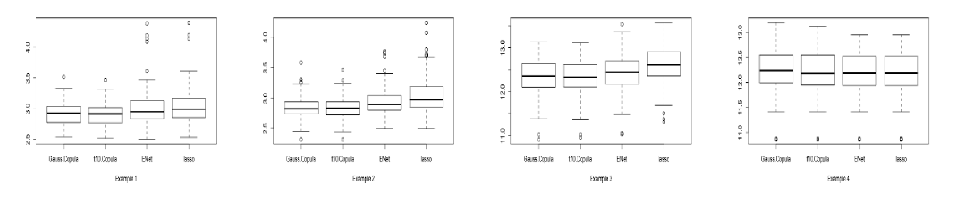
| Example 1 | Example 2 | Example 3 | Example 4 | |
|---|---|---|---|---|
| LGC | 2.92 (0.02) | 2.82 (0.020) | 12.35 (0.051) | 12.24 (0.07) |
| lasso Copula | 2.92 (0.02) | 2.83 (0.017) | 12.32 (0.048) | 12.18 (0.08) |
| Elastic net | 2.95 (0.03) | 2.89 (0.025) | 12.44 (0.068) | 12.19 (0.07) |
| lasso | 2.99 (0.02) | 2.97 (0.026) | 12.61 (0.043) | 12.19 (0.07) |

| Test set MSE | Tuning Parameter Estimates | Selected Features | |
|---|---|---|---|
| Lasso | 897.071 | = 5.59 | 6/10 |
| Elastic net | 871.368 | = 0.947, = 2.915 | 6/10 |
| Gaussian Copula | 856.693 | =0.458 | 10/10 |
| t Copula () | 857.576 | = 0.615 | 10/10 |
| Test set MCE | Tuning Parameter Estimates | Selected Features | |
|---|---|---|---|
| Lasso | 9/22 | =0.09 | 7/201 |
| Elastic net | 5/22 | =0 , =0.03 | 201/201 |
| Gaussian Copula | 5/22 | = 0.1 | 70/201 |
| Test set MSE | Tuning Parameter Estimates | Included Features | |
|---|---|---|---|
| Lasso | 0.699 | = 0.01 | 16/27 |
| Elastic net | 0.699 | = 0.21, = 0.03 | 18/27 |
| Gaussian Copula | 0.768 | = 0.14 | 4/27 |
5.1 Synthetic experiments
Here we present four examples from [25, 30], to compare the prediction performance of the lasso and EN and proposed copula prior. For each example, our simulated data consist of a training data set, an independent validation data set, and a separate test data set. The validation data sets were used to select the tuning parameters and then the models were fitted on the training data set. We computed the test error (the mean-squared error) on the test data set. The simulation scenarios are as follows:
- (a)
We consider the true model, , where we set , and , where
We simulated 100 data sets. Training set sample size = 20; Validation set sample size = 20; and Test set sample size = 200.
- (b)
Example 2 is the same as example 1, except that for all .
- (c)
In example 3, we consider the true model, , where we set
and and , where
We simulated 100 data sets with Training set sample size = 100; Validation set sample size = 100; and Test set sample size = 400.
- (d)
In example 4, we consider the true model, , where we set
and . Let , for , the predictors are generated from
We simulated 100 data sets with Training set sample size = 100; Validation set sample size = 100; and Test set sample size = 400.
Table 2 and figure 4 (box plots) summarize the prediction results. We see that in the examples 1, 2 and 3, based on RMSE, the ‘lasso with -copula’ and LGC tend to be more accurate than the lasso and the EN. While in example 4, the copula priors tend to do as well as the EN and lasso. This is expected because in example 4, predictors are not correlated and hence proposed copula priors will do as good as the regular lasso or the EN penalty.
5.2 Regression for Diabetes Data
The diabetes dataset arises from the study of 442 diabetes patients describes in the [10]. It comprises a sample of 442 diabetic patients. The independent variables are age, sex, body mass index (BMI), average blood pressure, and six blood serum measurements. The dependent variable is the quantitative measure of disease progression in one year after measuring the independent variables. For data analysis, we randomly split the data with 300 observations in the training set and the remaining 142 observations in the test set. We evaluate the MSE for copula prior, EN, and lasso on the test data set. The table (3) presents the results.
For choosing the optimal tuning parameters, we have used ten-fold cross-validation for all the above regularizers. The LGC prior selects all the variables in the final model. The unique solution path of LGC prior (presented in figure 5) is formed as it takes into account the correlation among the predictors. The regularization paths for lasso and EN for the diabetes dataset are reported in [26]. The six blood serum measurement variables (TC, LDL, HDL, TCH, LTG, GLU) are highly correlated with each other since they belong to the same person’s blood. The BMI and map variable also have a significant amount of correlation with other predictors. For all the three cases the regularization path for age and sex variable is similar, as the age and sex variable are not correlated with other predictors. However, the solution path of LGC prior changes concerning lasso prior, as the LGC prior takes into account the correlation among the predictors. As a result, it results in lower MSE than regular lasso and EN.
Both the EN and lasso select sex, BMI, MAP, HDL, LTG, and GLU to be the significant predictors. EN performs better than lasso due to the presence of ridge penalty but tends to perform worse than the copula prior. The lasso is a particular case of the LGC prior when the prior correlation among the predictors is assumed 0. We have used copula with 10 degrees of freedom. The optimal value in case of copula comes out to be 0.615. Again in the copula prior, the test data error is small, as compared with EN and lasso; copula selects all the variables in the final model.
5.3 Classification for Colon Cancer Data
Microarray data is a classic example of high dimensional data. The experiments on DNA, RNA and protein microarrays which consists of the expression state of a vast number of genes generates high dimensional data. There are often thousands of features (gene expression) for such data but very few samples. As a result, there is a need for feature selection in such type of data. The response variable often classified as the cancerous cell or healthy cell.
Here, we consider the example of the Colon cancer data set as explained in [1]. This dataset consists of 62 tissue samples collected from colon cancer patients. From these 62 samples, 40 biopsies are from tumors (labeled as “1”) and rest 22 biopsies (labeled as “0”) are from healthy parts of the colon of the same patients. Top 2000 features are selected from 6500 features based on the confidence in measured gene expression levels.
The goal is to develop a diagnostic rule based on the gene expression of 2000 genes to differentiate cancerous tissues from healthy tissues. For this classification problem, we fit a logistic regression on training data with LGC prior, as the regularizer function. After learning the coefficients on training data, we use these coefficients on test data to evaluate the misclassification error.
We divide the data into test and training data set. In the training dataset, there are 40 tissue samples of which 13 are the normal tissues, and rest 27 are tumor samples. The misclassification error is evaluated on the remaining 22 samples. Since the data has very high dimension, we first select top 200 predictors based on their statistic scores from training data. It helps us in making the computation easier.
The prior correlation matrix between coefficients learned from (16). Another unknown quantity is the scale parameter , which we learned from five-fold cross-validation method. Table (4) compares the out-sample misclassification error (MCE) of the LGC prior with other feature selection methods like lasso EN. The LGC prior has much lower MCE than lasso. Both LGC and EN have the same MCE, but LGC resulted in a sparse representation. The LGC selected only 70 features out of 201 features, whereas the EN selected all the features.
5.4 Large Time Series Data for Energy and Housing
The energy appliances dataset arises from the study of household energy uses from appliances describes in the [4]. The dataset is available for about 4.5 months at 10 minutes interval. The house temperature and humidity conditions were monitored with a wireless sensor network. The energy data was logged every 10 minutes. Weather data collected from the nearest airport weather station (Chievres Airport, Belgium) was downloaded from a public dataset and merged with the experimental datasets using the date and time column. Overall the data is a time series having 19735 observations and 27 features. We considered the first 3.15 month () as training data set, and the rest of dataset as the test dataset for measuring the performance of the model.
Since the data is a time series, we checked the stationarity of the variables involved. The Augmented Dickey-Fuller test confirms that all the variables involved are stationary. Hence we used regular linear time series model for feature selection.
As the size of data is large, we used the resampling technique defined in the algorithm (4). A small resample of size 1500 sampled with replacement from the training dataset and solutions obtained using (15). The process repeated for 200 times. As a result, we have 200 solutions. Finally, the median of these 200 solutions is considered as the final solution. For choosing the optimal tuning parameters, we used ten-fold cross-validation for all the regularizers. We evaluated the MSE for LGC, EN, and lasso on the test data set. The results presented in table (5). As evident from the table (5), the MSE for lasso,EN and LGC are similar. This is expected because in this data set predictors are only slightly correlated.
6 Conclusion
We presented the copula prior, a shrinkage and feature selection method. The LC prior produces a sparse model with good prediction accuracy while preserving the grouping effect. The empirical results and simulations demonstrate the better performance of the LC prior and its superiority over the EN and the lasso. When used in the binary classification method, the LC prior appears to perform well on microarray data regarding the misclassification error, and it makes automatic gene selection.
The LC prior is implemented in standard supervised learning task, like regression and classification. The copula prior is a generalization of the EN and lasso, which has been shown to be an essential device for model fitting and feature selection. Our method offers other insights into the lasso and EN, and ways to improve it.
Appendix A: Proof of Results on Copula Prior
Proof of Lemma 3.3: The objective function is
| (19) | |||||
From [18] we know that partial correlation satisfy the following relation, , where is the ols coefficient of the following regression equation , and is the R square value for this regression equation. By similar argument the partial correlation where is the ols coefficient of the following regression equation , and is the R square value for this regression equation. The ols coefficients satisfy the following linear equation.
| (20) | |||||
| (21) |
| (22) |
where j k,l. Equation (22) is satisfied only if j k,l. Similarly we can show that approaches as approaches . Consequently if then (. Q.E.D.
Proof of Lemma 3.4: Suppose is the optimal solution with . At the optimal point, and , so we have
| (23) | |||||
| (24) | |||||
Now we subtract (24) from (23) and using the result from Lemma 4.2 we have
| (25) | |||||
The equation (25) is trivially satisfied, if . Another possible root is , where we have the following condition,
| (26) |
Substitute (26) into (19) we have the following equation,
| (27) | |||||
Since is the optimal solution, then should be the minimum. Consider another solution . Since , then . Also . The only difference between the solution and the new solution would be the following,
| (28) |
The equation (28) takes a positive value by assumption (3.2)which implies that L, hence a contradiction. So Q.E.D.
Proof of Theorem 3.1: Suppose is the optimal solution with . At the optimal point, and , so we have
| (29) | |||
| (30) |
Subtract (30) from (29) and after some operations we get the following equation,
| (31) |
where,
by Cauchy-Schwarz inequality,
Note that are vectors. We have . By assumption (3.1) q is a concave function, so we can say that is bounded by (The derivative of at ). Substitute these developments in above equation to get the upper bound. Similarly due to concavity of q it is evident that , if we have . Finally, we can say . Q.E.D.
Related work
In this section we review the existing feature selection algorithms compare our proposed method with them. Lasso proposed by [25] is widely used for feature selection. Copula lasso prior is a multivariate extension of lasso prior which accounts for the correlation between the features. In fact the ‘lasso with Gauss copula prior’ reduces to the lasso prior when the correlation between the features is 0.
EN proposed by [27] also incorporates the correlation between the features through eigen vectors of data covariance matrix. It is a Bayesian hybrid model which discovers the correlated features through the eigen information extracted from the data. EN [30] uses a weighted combination of and norms to encourage a grouping effect, where strongly correlated variables tend to be in or out of the model together. However EN does not use the correlation information embedded in the data in contrast with copula prior. Copula function can be used to develop a multivariate version of the EN to capture the correlation information between the features. However in this paper we restrict ourselves to the LC prior.
Ordered weight (OWL) algorithm [29] is also capable of selecting correlated features. But it forces the features in the same group to have the same coefficient value which introduces bias in the model. [11] discuss a general penalty function on the model parameters for . It is known as the Bridge estimator. Lasso is a special case of Bridge estimator corresponding to . For the bridge penalty function becomes non convex.
[28] introduced the -prior. This prior replicates the covariance structure of the data. However it cannot produce sparse solutions. Multivariate laplace distribution in which covariance structure is identical to data covariance serves many useful purposes. First it can identify the correlated features due to its built-in correlation structure and secondly it has the ability to produce sparse solutions. However handling multivariate laplace distribution is computationally difficult, so we have used copula techniques to develop the multivariate distribution function for lasso.
Acknowledgment
Sourish Das’s work was partially supported by the Infosys Foundation grant to CMI.
References
- [1] Alon, A., Barkai, N., Notterman, D. A., Gish, K., Ybarra, S., Mack, D., and Levine, A. Broad patterns of gene expression revealed by clustering analysis of tumor and normal colon tissues probed by oligonucleotide arrays. Proc. Natl. Acad. Sci. USA 96 (1999), 6745–6750.
- [2] Birgin, E. G., and Martinez, J. M. Improving ultimate convergence of an augmented lagrangian method. Optimization Methods and Software 23, 2 (2008), 177–195.
- [3] Bühlmann, P., Rütimann, P., van de Geer, S., and Zhang, C.-H. Correlated variables in regression: clustering and sparse estimation. Journal of Statistical Planning and Inference 143, 11 (2013), 1835–1858.
- [4] Candanedo, L. M., Feldheim, V., and Deramaix, D. Data driven prediction models of energy use of appliances in a low-energy house. Energy and Buildings 140 (2017), 81–97.
- [5] Chandrashekar, G., and Sahin, F. A survey on feature selection methods. Computers and Electrical Engineering 40 (2014), 16–28.
- [6] Clayton, D. A model for association in bivariate life tables and its application in epidemiological studies of familial tendency in chronic disease incidence. Biometrika 65 (1978), 141–152.
- [7] Conn, A. R., Gould, N. I. M., and Toint, P. L. A globally convergent augmented lagrangian algorithm for optimization with general constraints and simple bounds. SIAM Journal of Numerical Analysis 28, 2 (1991), 545–572.
- [8] Das, S., and Dey, D. K. On bayesian inference for generalized multivariate gamma distribution. Statistics and Probability Letters 80 (2010), 1492–1499.
- [9] Demarta, S., and McNeil, A. J. The t copula and related copulas. International Statistical Review 73, 1 (2005), 111–129.
- [10] Efron, B., Hastie, T., Johnstone, I., and Tibshirani, R. Least angle regression. The Annals of Statistics 32 (2004), 407–409.
- [11] Frank, L. E., and Friedman, J. H. A statistical view of some chemometrics regression tools. Technometrics 35, 2 (1993), 109–135.
- [12] Frank, M. On the simultaneous associativity of f(x, y) and x + y - f(x, y). Aequationes Mathematicae 19 (1979), 194–226.
- [13] Gumbel, E. Bivariate exponential distributions. Journal of the American Statistical Association 55 (1960), 698–707.
- [14] Guyon, I., and Elisseeff, A. An introduction to variable and feature selection. Journal of Machine Learning Research 3 (2003), 1157–1182.
- [15] Hastie, T., Tibshirani, R., and Friedman, J. The Elements of Statistical Learning: Data Mining, Inference, and Prediction. Springer, 2008.
- [16] Khare, K., and Hobert, J. P. Geometric ergodicity of bayesian lasso. Electronic Journal of Statistics 7 (2013), 2150–2163.
- [17] Kotz, S., Kozubowski, T. J., and Krzysztof, P. The Laplace Distribution and Generalizations. Birkhauser, 2001.
- [18] Kwan, C. C. A regression-based interpretation of the inverse of the sample covariance matrix. Spreadsheets in Education (eJSiE) 7, 1 (2014), 3.
- [19] Kyung, M., Gill, J., Ghosh, M., and Casella, G. Penalized regression, standard errors, and bayesian lassos. Bayesian Analysis 5 (2010), 369–412.
- [20] Li, Q., and Lin, N. The bayesian elastic net. Bayesian Analysis 5 (2010), 151–170.
- [21] Park, T., and Casella, G. The bayesian lasso. Journal of the American Statistical Association 103 (2008), 681–686.
- [22] Roy, V., and Chakraborty, S. Selection of tuning parameters, solution paths and standard errors for bayesian lassos. Bayesian Analysis 12, 3 (2017), 753–778.
- [23] Sklar, A. Fonctions de répartition à n dimensions et leurs marges. Publ. Inst. Statist. Univ. Paris 8 (1959), 229–231.
- [24] Song, P. Multivariate dispersion models generated from gaussian copula. Scandinavian Journal of Statistics 27, 2 (2000), 305–320.
- [25] Tibshirani, R. Regression shrinkage and selection via the lasso. Journal of the Royal Statistical Society, Series B 58 (1996), 267–288.
- [26] Vidaurre, D., Bielza, C., and Larrañaga, P. A survey of l1 regression. International Statistical Review 81, 3 (2013), 361–387.
- [27] Yan, F., and Qi, Y. Eigennet: A bayesian hybrid of generative and conditional models for sparse learning. In Advances in Neural Information Processing Systems (2011), pp. 2663–2671.
- [28] Zellner, A. On assessing prior distributions and bayesian regression analysis with g prior distributions. In Bayesian Inference and Decision Techniques: Essays in Honor of Bruno de Finetti, Studies in Bayesian Econometrics., P. Goel and A. Zellner, Eds. Elsevier, New York, 1986, ch. 6, pp. 233–243.
- [29] Zeng, X., and Figueiredo, M. A. The ordered weighted norm: Atomic formulation, projections, and algorithms.
- [30] Zou, H., and Hastie, T. Regularization and variable selection via the elastic net. Journal of the Royal Statistical Society, Series B 67 (2005), 301–320.