跳到论文正文
W Papers独立论文阅读器 arXiv:1709.05082 论文正文 计算阅读时间 · 0%
引用这篇论文根据当前论文元数据生成,正式投稿前建议核对。


License: CC BY 4.0
arXiv:1709.05082v1 [hep-ph] 15 Sep 2017

Υ⁡(n​S){\Upsilon}(nS) →{\to} Bc∗​DB_{c}^{\ast}D decays with perturbative QCD approach

Yueling Yang Affiliation: Institute of Particle and Nuclear Physics, Henan Normal University, Xinxiang 453007, China    Junfeng Sun Affiliation: Institute of Particle and Nuclear Physics, Henan Normal University, Xinxiang 453007, China    Jinshu Huang Affiliation: College of Physics and Electronic Engineering, Nanyang Normal University, Nanyang 473061, China    Haiyan Li Affiliation: Institute of Particle and Nuclear Physics, Henan Normal University, Xinxiang 453007, China    Gongru Lu Affiliation: Institute of Particle and Nuclear Physics, Henan Normal University, Xinxiang 453007, China    Qin Chang Affiliation: Institute of Particle and Nuclear Physics, Henan Normal University, Xinxiang 453007, China
Abstract

The Υ⁡(n​S){\Upsilon}(nS) →{\to} Bc∗​DB_{c}^{\ast}D weak decays (nn == 11, 22, 33) are investigated with perturbative QCD approach. It is found that the CKM-favored Υ⁡(n​S){\Upsilon}(nS) →{\to} Bc∗​DsB_{c}^{\ast}D_{s} decays have branching ratio of 𝒪⁡(10−10){\cal O}(10^{-10}), which might be potentially accessible to the future LHC and SuperKEKB experiments.

pacs
13.25.Gv 12.39.St 14.40.Pq

I Introduction

Υ⁡(1​S){\Upsilon}(1S), Υ⁡(2​S){\Upsilon}(2S) and Υ⁡(3​S){\Upsilon}(3S) are spin-triplet SS-wave b​b¯b\bar{b} bound states carrying with quantum number of IG​JP​CI^{G}J^{PC} == 0−​1−⁣−0^{-}1^{--} [1]. They all lie below the open bottom threshold. They must strongly decay into two light hadrons via b​b¯b\bar{b} annihilation into at least three gluons. So their decay width is very narrow, only dozens of keV. [Hereinafter, for simplicity sake, we will use a notation Υ⁡(n​S){\Upsilon}(nS) to represent Υ⁡(1​S){\Upsilon}(1S), Υ⁡(2​S){\Upsilon}(2S), and Υ⁡(3​S){\Upsilon}(3S) mesons.] Since their discovery in 1977 [2, 3], Υ⁡(n​S){\Upsilon}(nS) has been attracting much attention from experimentalists and theorists. Thanks to the excellent performance from experimental groups of CLEO, BaBar, Belle, CDF, D0, LHCb, ATLAS and so on, remarkable achievements have been made in understanding of the nature of upsilon [1, 4]. The strong and electromagnetic Υ⁡(n​S){\Upsilon}(nS) decay modes have been carefully investigated. With accumulation of Υ⁡(n​S){\Upsilon}(nS) data samples, it might be possible to search for Υ⁡(n​S){\Upsilon}(nS) weak decay at future LHC and SuperKEKB experiments.

Theoretically, both valence quarks of Υ⁡(n​S){\Upsilon}(nS) can decay individually via the weak interaction. The bb →{\to} cc transition is particularly favored by a hierarchy of the Cabibbo-Kabayashi-Maskawa (CKM) matrix elements. So Υ⁡(n​S){\Upsilon}(nS) decay into final states containing a Bc(∗)B_{c}^{(\ast)} meson should, in principle, have a relatively large branching fraction among its weak decay modes. Recently, some phenomenological QCD-inspired methods have been vividly developed to deal with heavy quark weak decay, such as perturbative QCD (pQCD) approach [5, 6, 7], QCD factorization (QCDF) [8, 9, 10, 11, 12] and soft and collinear effective theory [13, 14, 15, 16]. The Υ⁡(n​S){\Upsilon}(nS) →{\to} Bc∗​DB_{c}^{\ast}D decays offer a good plaza to ulteriorly test various phenomenological models and to further explore the underlying dynamical mechanism of heavy quarkonium weak decay. In addition, as far as we know, there is no experimental measurement report and few theoretical work related to Υ⁡(n​S){\Upsilon}(nS) →{\to} Bc∗​DB_{c}^{\ast}D decay for the moment. Herein, we will study the bottom- and charm-changing Υ⁡(n​S){\Upsilon}(nS) →{\to} Bc∗​DB_{c}^{\ast}D weak decays with pQCD approach to provide future experimental exploration with a useful reference.

This paper is organized as follows. The section II devotes to theoretical framework and amplitudes for Υ⁡(n​S){\Upsilon}(nS) →{\to} Bc∗​DB_{c}^{\ast}D decay. The numerical results and discussion are presented in section III. We summarize in the last section.

II theoretical framework

II.1 The effective Hamiltonian

The effective weak Hamiltonian describing nonleptonic Υ⁡(n​S){\Upsilon}(nS) →{\to} Bc∗​DB_{c}^{\ast}D decays is written as [17]

ℋeff=GF2​{Vc​b​Vc​q∗​∑i=12Ci​(μ)​Qi​(μ)−Vt​b​Vt​q∗​∑j=310Cj​(μ)​Qj​(μ)}+h.c.,{\cal H}_{\rm eff}\ =\ \frac{G_{F}}{\sqrt{2}}\,\Big\{V_{cb}V_{cq}^{\ast}\sum\limits_{i=1}^{2}C_{i}({\mu})\,Q_{i}({\mu})-V_{tb}V_{tq}^{\ast}\sum\limits_{j=3}^{10}C_{j}({\mu})\,Q_{j}({\mu})\Big\}+{\rm h.c.}, (1)

where GFG_{F} ≃{\simeq} 1.166×10⁻⁵​GeV−21.166{\times}10^{-5}\,{\rm GeV}^{-2} is the Fermi constant [1]; qq == dd and ss; the CKM factors can be expressed as

Vc​b​Vc​s∗\displaystyle V_{cb}V_{cs}^{\ast} =\displaystyle= +A​λ2−12​A​λ4−18​A​λ6​(1+4​A2)+𝒪⁡(λ7),\displaystyle+A{\lambda}^{2}-\frac{1}{2}A{\lambda}^{4}-\frac{1}{8}A{\lambda}^{6}(1+4A^{2})+{\cal O}({\lambda}^{7}), (2)
Vt​b​Vt​s∗\displaystyle V_{tb}V_{ts}^{\ast} =\displaystyle= −Vc​b​Vc​s∗−A​λ4​(ρ−i​η)+𝒪⁡(λ7),\displaystyle-V_{cb}V_{cs}^{\ast}-A{\lambda}^{4}({\rho}-i{\eta})+{\cal O}({\lambda}^{7}), (3)

for Υ⁡(n​S){\Upsilon}(nS) →{\to} Bc∗​DsB_{c}^{{\ast}}D_{s} decays; and

Vc​b​Vc​d∗\displaystyle V_{cb}V_{cd}^{\ast} =\displaystyle= −A​λ3+𝒪⁡(λ7),\displaystyle-A{\lambda}^{3}+{\cal O}({\lambda}^{7}), (4)
Vt​b​Vt​d∗\displaystyle V_{tb}V_{td}^{\ast} =\displaystyle= +A​λ3​(1−ρ+i​η)+12​A​λ5​(ρ−i​η)+𝒪⁡(λ7),\displaystyle+A{\lambda}^{3}(1-{\rho}+i{\eta})+\frac{1}{2}A{\lambda}^{5}({\rho}-i{\eta})+{\cal O}({\lambda}^{7}), (5)

for Υ⁡(n​S){\Upsilon}(nS) →{\to} Bc(∗)​DdB_{c}^{({\ast})}D_{d} decays; AA, λ{\lambda}, ρ{\rho} and η{\eta} are Wolfenstein parameters [1, 18].

The local tree operators Q1,2Q_{1,2}, QCD penguin operators Q3,⋯,6Q_{3,{\cdots},6}, and electroweak operators Q7,⋯,10Q_{7,{\cdots},10} are defined below.

Q1\displaystyle Q_{1} =\displaystyle= [c¯α​γμ​(1−γ5)​bα]​[q¯β​γμ​(1−γ5)​cβ],\displaystyle[\bar{c}_{\alpha}{\gamma}_{\mu}(1-{\gamma}_{5})b_{\alpha}][\bar{q}_{\beta}{\gamma}^{\mu}(1-{\gamma}_{5})c_{\beta}], (6)
Q2\displaystyle Q_{2} =\displaystyle= [c¯α​γμ​(1−γ5)​bβ]​[q¯β​γμ​(1−γ5)​cα],\displaystyle[\bar{c}_{\alpha}{\gamma}_{\mu}(1-{\gamma}_{5})b_{\beta}][\bar{q}_{\beta}{\gamma}^{\mu}(1-{\gamma}_{5})c_{\alpha}], (7)
Q3\displaystyle Q_{3} =\displaystyle= ∑q′[q¯α​γμ​(1−γ5)​bα]​[q¯β′​γμ​(1−γ5)​qβ′],\displaystyle\sum\limits_{q^{\prime}}[\bar{q}_{\alpha}{\gamma}_{\mu}(1-{\gamma}_{5})b_{\alpha}][\bar{q}^{\prime}_{\beta}{\gamma}^{\mu}(1-{\gamma}_{5})q^{\prime}_{\beta}], (8)
Q4\displaystyle Q_{4} =\displaystyle= ∑q′[q¯α​γμ​(1−γ5)​bβ]​[q¯β′​γμ​(1−γ5)​qα′],\displaystyle\sum\limits_{q^{\prime}}[\bar{q}_{\alpha}{\gamma}_{\mu}(1-{\gamma}_{5})b_{\beta}][\bar{q}^{\prime}_{\beta}{\gamma}^{\mu}(1-{\gamma}_{5})q^{\prime}_{\alpha}], (9)
Q5\displaystyle Q_{5} =\displaystyle= ∑q′[q¯α​γμ​(1−γ5)​bα]​[q¯β′​γμ​(1+γ5)​qβ′],\displaystyle\sum\limits_{q^{\prime}}[\bar{q}_{\alpha}{\gamma}_{\mu}(1-{\gamma}_{5})b_{\alpha}][\bar{q}^{\prime}_{\beta}{\gamma}^{\mu}(1+{\gamma}_{5})q^{\prime}_{\beta}], (10)
Q6\displaystyle Q_{6} =\displaystyle= ∑q′[q¯α​γμ​(1−γ5)​bβ]​[q¯β′​γμ​(1+γ5)​qα′],\displaystyle\sum\limits_{q^{\prime}}[\bar{q}_{\alpha}{\gamma}_{\mu}(1-{\gamma}_{5})b_{\beta}][\bar{q}^{\prime}_{\beta}{\gamma}^{\mu}(1+{\gamma}_{5})q^{\prime}_{\alpha}], (11)
Q7\displaystyle Q_{7} =\displaystyle= ∑q′32​eq′​[q¯α​γμ​(1−γ5)​bα]​[q¯β′​γμ​(1+γ5)​qβ′],\displaystyle\sum\limits_{q^{\prime}}\frac{3}{2}e_{q^{\prime}}\,[\bar{q}_{\alpha}{\gamma}_{\mu}(1-{\gamma}_{5})b_{\alpha}][\bar{q}^{\prime}_{\beta}{\gamma}^{\mu}(1+{\gamma}_{5})q^{\prime}_{\beta}], (12)
Q8\displaystyle Q_{8} =\displaystyle= ∑q′32​eq′​[q¯α​γμ​(1−γ5)​bβ]​[q¯β′​γμ​(1+γ5)​qα′],\displaystyle\sum\limits_{q^{\prime}}\frac{3}{2}e_{q^{\prime}}\,[\bar{q}_{\alpha}{\gamma}_{\mu}(1-{\gamma}_{5})b_{\beta}][\bar{q}^{\prime}_{\beta}{\gamma}^{\mu}(1+{\gamma}_{5})q^{\prime}_{\alpha}], (13)
Q9\displaystyle Q_{9} =\displaystyle= ∑q′32​eq′​[q¯α​γμ​(1−γ5)​bα]​[q¯β′​γμ​(1−γ5)​qβ′],\displaystyle\sum\limits_{q^{\prime}}\frac{3}{2}e_{q^{\prime}}\,[\bar{q}_{\alpha}{\gamma}_{\mu}(1-{\gamma}_{5})b_{\alpha}][\bar{q}^{\prime}_{\beta}{\gamma}^{\mu}(1-{\gamma}_{5})q^{\prime}_{\beta}], (14)
Q10\displaystyle Q_{10} =\displaystyle= ∑q′32​eq′​[q¯α​γμ​(1−γ5)​bβ]​[q¯β′​γμ​(1−γ5)​qα′],\displaystyle\sum\limits_{q^{\prime}}\frac{3}{2}e_{q^{\prime}}\,[\bar{q}_{\alpha}{\gamma}_{\mu}(1-{\gamma}_{5})b_{\beta}][\bar{q}^{\prime}_{\beta}{\gamma}^{\mu}(1-{\gamma}_{5})q^{\prime}_{\alpha}], (15)

where α{\alpha} and β{\beta} are color indices; q′q^{\prime} == uu, dd, ss, cc, bb has an electric charge eq′e_{q^{\prime}} in the unit of |e|{|}e{|}.

The scale μ{\mu} separates physical contributions into two components. The Wilson coefficients Ci​(μ)C_{i}(\mu) summarize the physical contributions above μ{\mu}, and has been reliably computed to the next-to-leading order with perturbation theory [17]. The hadronic matrix elements (HME), where the local operators are sandwiched between initial and final hadron states, contain the physical contributions below μ{\mu}. Due to the incorporation of long distance contributions and the entanglement of perturbative and nonperturbative effects, HME is not yet fully understood until now. However, in order to evaluate the amplitudes, one has to face directly the HME’s calculation based on some approximation and assumptions, which leads to large theoretical uncertainties.

II.2 Hadronic matrix elements

Phenomenologically, combining factorization hypothesis [19, 20, 21] and hard-scattering approach [22, 23, 24, 25, 26], HME could be written as the convolution of hard scattering kernel function 𝒯{\cal T} and distribution amplitudes (DAs) of participating hadrons. DAs are nonperturbative but universal inputs, which can be obtained from nonperturbative methods or fitted from experimental data. In order to eliminate the endpoint singularities accompanying with spectator rescattering and annihilation contributions based on a collinear approximation [10, 11, 12], and in the meantime to provide an effective cutoff on nonperturbative contributions, the transverse momentum of valence quarks is kept explicitly and a Sudakov factor for each of DAs is introduced compulsorily with pQCD approach [5, 6, 7]. A general pQCD amplitude is made up of three parts: the Wilson coefficients CiC_{i} absorbing physical contributions above a typical scale of tt, hard scattering kernel function 𝒯{\cal T} accounting for heavy quark weak decay, and wave functions Φ{\Phi}, i.e.,

∫d​k​Ci​(t)​𝒯​(t,k)​∏jΦj​(k)​e−Sj,{\int}dk\,C_{i}(t)\,{\cal T}(t,k)\,\prod_{j}{\Phi}_{j}(k)\,e^{-S_{j}}, (16)

where kk is the momentum of valence quarks, and e−Sje^{-S_{j}} is a Sudakov factor.

II.3 Kinematic variables

In the Υ⁡(n​S){\Upsilon}(nS) rest frame, the light cone kinematic variables are defined as follows.

pΥ=p1=m12​(1,1,0),p_{\Upsilon}\,=\,p_{1}\,=\,\frac{m_{1}}{\sqrt{2}}(1,1,0), (17)
pBc∗=p2=(p2+,p2−,0),p_{B_{c}^{\ast}}\,=\,p_{2}\,=\,(p_{2}^{+},p_{2}^{-},0), (18)
pD=p3=(p3−,p3+,0),p_{D}\,=\,p_{3}\,=\,(p_{3}^{-},p_{3}^{+},0), (19)
pi±=(Ei±p)/2,p_{i}^{\pm}\,=\,(E_{i}\,{\pm}\,p)/\sqrt{2}, (20)
ki=xi​pi+(0,0,k→i​T),k_{i}\,=\,x_{i}\,p_{i}+(0,0,\vec{k}_{iT}), (21)
ϵ1∥=p1m1−m1p1⋅n+​n+,{\epsilon}_{1}^{\parallel}\,=\,\frac{p_{1}}{m_{1}}-\frac{m_{1}}{p_{1}{\cdot}n_{+}}n_{+}, (22)
ϵ2∥=p2m2−m2p2⋅n−​n−,{\epsilon}_{2}^{\parallel}\,=\,\frac{p_{2}}{m_{2}}-\frac{m_{2}}{p_{2}{\cdot}n_{-}}n_{-}, (23)
ϵ1,2⟂=(0,0,1→),{\epsilon}_{1,2}^{\perp}\,=\,(0,0,\vec{1}), (24)
n+=(1,0,0),n_{+}=(1,0,0), (25)
n−=(0,1,0),n_{-}=(0,1,0), (26)
s= 2​p2⋅p3=m12−m22−m32,s\,=\,2\,p_{2}{\cdot}p_{3}\,=\,m_{1}^{2}-m_{2}^{2}-m_{3}^{2}, (27)
t= 2​p1⋅p2=m12+m22−m32= 2​m1​E2,t\,=\,2\,p_{1}{\cdot}p_{2}\,=\,m_{1}^{2}+m_{2}^{2}-m_{3}^{2}\,=\,2\,m_{1}\,E_{2}, (28)
u= 2​p1⋅p3=m12−m22+m32= 2​m1​E3,u\,=\,2\,p_{1}{\cdot}p_{3}\,=\,m_{1}^{2}-m_{2}^{2}+m_{3}^{2}\,=\,2\,m_{1}\,E_{3}, (29)
u+t−s=m12+m22+m32,u+t-s\,=\,m_{1}^{2}+m_{2}^{2}+m_{3}^{2}, (30)
s​t+s​u−t​u−4​m12​p2= 0,s\,t+s\,u-t\,u-4\,m_{1}^{2}\,p^{2}\,=\,0, (31)

where xix_{i} and ki​Tk_{iT} are the longitudinal momentum fraction and transverse momentum of valence quark, respectively; ϵi∥{\epsilon}_{i}^{\parallel} and ϵi⟂{\epsilon}_{i}^{\perp} are the longitudinal and transverse polarization vectors, respectively, satisfying relations ϵi2{\epsilon}_{i}^{2} == −1-1 and ϵi⋅pi{\epsilon}_{i}{\cdot}p_{i} == 00; the subscript ii == 11, 22, 33 on variables (EiE_{i}, pip_{i}, mim_{i}, ϵi{\epsilon}_{i}) corresponds to Υ⁡(n​S){\Upsilon}(nS), Bc∗B_{c}^{\ast}, and DD mesons, respectively; n+n_{+} and n−n_{-} are the positive and negative null vectors, respectively; ss, tt and uu are Lorentz-invariant variables. These kinematic variables are showed in Fig.2(a).

II.4 Wave functions

The definitions of wave functions are [27, 28],

⟨0|bi(z)b¯j(0)|Υ(p1,ϵ1∥)⟩=fΥ4∫dk1e−ik1⋅z{ϵ̸1∥[m1ϕΥv(k1)−p̸1ϕΥt(k1)]}j​i,{\langle}0{|}b_{i}(z)\bar{b}_{j}(0){|}{\Upsilon}(p_{1},{\epsilon}_{1}^{{\parallel}}){\rangle}\,=\,\frac{f_{{\Upsilon}}}{4}{\int}dk_{1}\,e^{-ik_{1}{\cdot}z}\Big\{\!\!\not{\epsilon}_{1}^{{\parallel}}\Big[m_{1}\,{\phi}_{\Upsilon}^{v}(k_{1})-\!\!\not{p}_{1}\,{\phi}_{\Upsilon}^{t}(k_{1})\Big]\Big\}_{ji}, (32)
⟨0|bi(z)b¯j(0)|Υ(p1,ϵ1⟂)⟩=fΥ4∫dk1e−ik1⋅z{ϵ̸1⟂[m1ϕΥV(k1)−p̸1ϕΥT(k1)]}j​i,{\langle}0{|}b_{i}(z)\bar{b}_{j}(0){|}{\Upsilon}(p_{1},{\epsilon}_{1}^{{\perp}}){\rangle}\,=\,\frac{f_{{\Upsilon}}}{4}{\int}dk_{1}\,e^{-ik_{1}{\cdot}z}\Big\{\!\!\not{\epsilon}_{1}^{{\perp}}\Big[m_{1}\,{\phi}_{\Upsilon}^{V}(k_{1})-\!\!\not{p}_{1}\,{\phi}_{\Upsilon}^{T}(k_{1})\Big]\Big\}_{ji}, (33)
⟨Bc∗​(p2,ϵ2∥)|c¯i​(z)​bj​(0)|0⟩=fBc∗4​∫01d​k3​ei​k2⋅z​{ϵ̸2∥​[m2​ϕBc∗v​(k2)+p̸2​ϕBc∗t​(k2)]}j​i,{\langle}B_{c}^{\ast}(p_{2},{\epsilon}_{2}^{{\parallel}}){|}\bar{c}_{i}(z)b_{j}(0){|}0{\rangle}\ =\ \frac{f_{B_{c}^{\ast}}}{4}{\int}_{0}^{1}dk_{3}\,e^{ik_{2}{\cdot}z}\Big\{\!\not{\epsilon}_{2}^{{\parallel}}\Big[m_{2}\,{\phi}_{B_{c}^{\ast}}^{v}(k_{2})+\!\not{p}_{2}\,{\phi}_{B_{c}^{\ast}}^{t}(k_{2})\Big]\Big\}_{ji}, (34)
⟨Bc∗​(p2,ϵ2⟂)|c¯i​(z)​bj​(0)|0⟩=fBc∗4​∫01d​k2​ei​k2⋅z​{ϵ̸2⟂​[m2​ϕBc∗V​(k2)+p̸2​ϕBc∗T​(k2)]}j​i,{\langle}B_{c}^{{\ast}}(p_{2},{\epsilon}_{2}^{{\perp}}){|}\bar{c}_{i}(z)b_{j}(0){|}0{\rangle}\ =\ \frac{f_{B_{c}^{\ast}}}{4}{\int}_{0}^{1}dk_{2}\,e^{ik_{2}{\cdot}z}\Big\{\!\not{\epsilon}_{2}^{{\perp}}\Big[m_{2}\,{\phi}_{B_{c}^{\ast}}^{V}(k_{2})+\!\not{p}_{2}\,{\phi}_{B_{c}^{\ast}}^{T}(k_{2})\Big]\Big\}_{ji}, (35)
⟨D⁡(p3)|ci​(0)​q¯j​(z)|0⟩=i​fD4​∫d​k3​ei​k3⋅z​{γ5​[p̸3​ϕDa​(k3)+m3​ϕDp​(k3)]}j​i,{\langle}D(p_{3}){|}c_{i}(0)\bar{q}_{j}(z){|}0{\rangle}\,=\,\frac{i\,f_{D}}{4}{\int}dk_{3}\,e^{ik_{3}{\cdot}z}\,\Big\{{\gamma}_{5}\Big[\!\!\not{p}_{3}\,{\phi}_{D}^{a}(k_{3})+m_{3}\,{\phi}_{D}^{p}(k_{3})\Big]\Big\}_{ji}, (36)

where fΥf_{\Upsilon}, fBc∗f_{B_{c}^{\ast}}, fDf_{D} are decay constants; wave functions ΦΥ,Bc∗v,T{\Phi}_{{\Upsilon},B_{c}^{\ast}}^{v,T} and ΦDa{\Phi}_{D}^{a} are twist-2; ΦΥ,Bc∗t,V{\Phi}_{{\Upsilon},B_{c}^{\ast}}^{t,V} and ΦDp{\Phi}_{D}^{p} are twist-3. The explicit expressions of DAs are [29]

ϕΥv​(x)=ϕΥT​(x)=A1​x​x¯​exp⁡{−mb28​ω12​x​x¯},{\phi}_{\Upsilon}^{v}(x)={\phi}_{\Upsilon}^{T}(x)=A_{1}\,x\bar{x}\,{\exp}\Big\{-\frac{m_{b}^{2}}{8\,{\omega}_{1}^{2}\,x\,\bar{x}}\Big\}, (37)
ϕΥt​(x)=A2​(x¯−x)2​exp⁡{−mb28​ω12​x​x¯},{\phi}_{\Upsilon}^{t}(x)=A_{2}\,(\bar{x}-x)^{2}\,{\exp}\Big\{-\frac{m_{b}^{2}}{8\,{\omega}_{1}^{2}\,x\,\bar{x}}\Big\}, (38)
ϕΥV​(x)=A3​{1+(x¯−x)2}​exp⁡{−mb28​ω12​x​x¯},{\phi}_{\Upsilon}^{V}(x)=A_{3}\,\Big\{1+(\bar{x}-x)^{2}\Big\}\,{\exp}\Big\{-\frac{m_{b}^{2}}{8\,{\omega}_{1}^{2}\,x\,\bar{x}}\Big\}, (39)
ϕΥ⁡(2​S)v,t,T,V​(x)=Bi​ϕΥ⁡(1​S)v,t,T,V​(x)​{1+mb22​ω12​x​x¯},{\phi}_{{\Upsilon}(2S)}^{v,t,T,V}(x)=B_{i}\,{\phi}_{{\Upsilon}(1S)}^{v,t,T,V}(x)\,\Big\{1+\frac{m_{b}^{2}}{2\,{\omega}_{1}^{2}\,x\,\bar{x}}\Big\}, (40)
ϕΥ⁡(3​S)v,t,T,V​(x)=Ci​ϕΥ⁡(1​S)v,t,T,V​(x)​{(1−mb22​ω12​x​x¯)2+6},{\phi}_{{\Upsilon}(3S)}^{v,t,T,V}(x)=C_{i}\,{\phi}_{{\Upsilon}(1S)}^{v,t,T,V}(x)\,\Big\{\Big(1-\frac{m_{b}^{2}}{2\,{\omega}_{1}^{2}\,x\,\bar{x}}\Big)^{2}+6\Big\}, (41)
ϕBc∗v​(x)=ϕBc∗T​(x)=D1​x​x¯​exp⁡{−x¯​mc2+x​mb28​ω22​x​x¯},{\phi}_{B_{c}^{\ast}}^{v}(x)={\phi}_{B_{c}^{\ast}}^{T}(x)=D_{1}\,x\bar{x}\,{\exp}\Big\{-\frac{\bar{x}\,m_{c}^{2}+x\,m_{b}^{2}}{8\,{\omega}_{2}^{2}\,x\,\bar{x}}\Big\}, (42)
ϕBc∗t​(x)=D2​(x¯−x)2​exp⁡{−x¯​mc2+x​mb28​ω22​x​x¯},{\phi}_{B_{c}^{\ast}}^{t}(x)=D_{2}\,(\bar{x}-x)^{2}\,{\exp}\Big\{-\frac{\bar{x}\,m_{c}^{2}+x\,m_{b}^{2}}{8\,{\omega}_{2}^{2}\,x\,\bar{x}}\Big\}, (43)
ϕBc∗V​(x)=D3​{1+(x¯−x)2}​exp⁡{−x¯​mc2+x​mb28​ω22​x​x¯},{\phi}_{B_{c}^{\ast}}^{V}(x)=D_{3}\,\Big\{1+(\bar{x}-x)^{2}\Big\}\,{\exp}\Big\{-\frac{\bar{x}\,m_{c}^{2}+x\,m_{b}^{2}}{8\,{\omega}_{2}^{2}\,x\,\bar{x}}\Big\}, (44)
ϕDa​(x)=E1​x​x¯​exp⁡{−x¯​mq2+x​mc28​ω32​x​x¯},{\phi}_{D}^{a}(x)=E_{1}\,x\bar{x}\,{\exp}\Big\{-\frac{\bar{x}\,m_{q}^{2}+x\,m_{c}^{2}}{8\,{\omega}_{3}^{2}\,x\,\bar{x}}\Big\}, (45)
ϕDp​(x)=E2​exp⁡{−x¯​mq2+x​mc28​ω32​x​x¯},{\phi}_{D}^{p}(x)=E_{2}\,{\exp}\Big\{-\frac{\bar{x}\,m_{q}^{2}+x\,m_{c}^{2}}{8\,{\omega}_{3}^{2}\,x\,\bar{x}}\Big\}, (46)

where x¯\bar{x} == 11 −- xx; parameter ωi{\omega}_{i} == mi​αs​(mi)m_{i}\,{\alpha}_{s}(m_{i}) determines the average transverse quark momentum according to nonrelativistic quantum chromodynamics (NRQCD) power counting rules [30]; parameters AiA_{i}, BiB_{i}, CiC_{i}, DiD_{i}, EiE_{i} are normalization coefficients,

∫01d​x​ϕΥi​(x)=1,fori=v,t,V,T,{\int}_{0}^{1}dx\,{\phi}_{\Upsilon}^{i}(x)=1,\quad\text{for}\ \ i=v,t,V,T, (47)
∫01d​x​ϕBc∗i​(x)=1,fori=v,t,V,T,{\int}_{0}^{1}dx\,{\phi}_{B_{c}^{\ast}}^{i}(x)=1,\quad\text{for}\ \ i=v,t,V,T, (48)
∫01d​x​ϕDi​(x)=1,fori=a,p.{\int}_{0}^{1}dx\,{\phi}_{D}^{i}(x)=1,\quad\text{for}\ \ i=a,p. (49)
Refer to caption
Figure 1: The normalized distribution amplitudes for Υ⁡(n​S){\Upsilon}(nS), Bc∗B_{c}^{\ast}, DD mesons.

The shape lines of DAs for Υ⁡(n​S){\Upsilon}(nS), Bc∗B_{c}^{\ast}, DD mesons are displayed in Fig.1. It is clearly seen that DAs fall quickly down to zero at endpoint xx, x¯\bar{x} →{\to} 00 due to suppression from exponential functions, which offer a natural cutoff for soft contributions.

Refer to caption
Figure 2: Feynman diagrams for Υ⁡(n​S){\Upsilon}(nS) →{\to} Bc∗​DsB_{c}^{\ast}D_{s} decay with pQCD approach, where (a,b) are factorizable emission diagrams, (c,d) are nonfactorizable emission diagrams, (e,f) are nonfactorizable annihilation diagrams, and (g,h) are factorizable annihilation diagrams.

II.5 Decay amplitudes

The Feynman diagrams for Υ⁡(n​S){\Upsilon}(nS) →{\to} Bc∗​DsB_{c}^{\ast}D_{s} decay are showed in Fig.2. There are two types. One is emission topology, and the other is annihilation topology. Each type is further subdivided into factorizable and nonfactorizable diagrams.

After a detail calculation, amplitude for Υ⁡(n​S){\Upsilon}(nS) →{\to} Bc∗​DB_{c}^{\ast}D decay is written as

𝒜⁡(Υ→Bc∗​D)=𝒜L​(ϵ1∥,ϵ2∥)+𝒜N​(ϵ1⟂⋅ϵ2⟂)+i​𝒜T​εμ​ν​α​β​ϵ1μ​ϵ2ν​p1α​p2β,{\cal A}({\Upsilon}{\to}B_{c}^{\ast}D)\ =\ {\cal A}_{L}({\epsilon}_{1}^{{\parallel}},{\epsilon}_{2}^{{\parallel}})+{\cal A}_{N}({\epsilon}_{1}^{{\perp}}{\cdot}{\epsilon}_{2}^{{\perp}})+i\,{\cal A}_{T}\,{\varepsilon}_{{\mu}{\nu}{\alpha}{\beta}}\,{\epsilon}_{1}^{{\mu}}\,{\epsilon}_{2}^{{\nu}}\,p_{1}^{\alpha}\,p_{2}^{\beta}, (50)

which is also written as the helicity amplitudes,

ℳ0=−𝒞​𝒜L​(ϵ1∥,ϵ2∥),{\cal M}_{0}\ =\ -{\cal C}\,{\cal A}_{L}({\epsilon}_{1}^{{\parallel}},{\epsilon}_{2}^{{\parallel}}), (51)
ℳ∥=2​𝒞​𝒜N,{\cal M}_{\parallel}\ =\ \sqrt{2}\,{\cal C}\,{\cal A}_{N}, (52)
ℳ⟂=2​𝒞​m1​p​𝒜T,{\cal M}_{\perp}\ =\ \sqrt{2}\,{\cal C}\,m_{1}\,p\,{\cal A}_{T}, (53)
𝒞=i​GF2​CFNc​π​fΥ​fBc∗​fD,{\cal C}\ =\ i\frac{G_{F}}{\sqrt{2}}\,\frac{C_{F}}{N_{c}}\,{\pi}\,f_{{\Upsilon}}\,f_{B_{c}^{\ast}}\,f_{D}, (54)

where CFC_{F} == 4/34/3 and the color number NcN_{c} == 33.

The expression of polarization amplitude 𝒜j{\cal A}_{j} is

𝒜j\displaystyle{\cal A}_{j} =\displaystyle= Vc​b​Vc​q∗​{(𝒜a,jL​L+𝒜b,jL​L)​a1+(𝒜c,jL​L+𝒜d,jL​L)​C2}\displaystyle V_{cb}V_{cq}^{\ast}\,\Big\{\Big({\cal A}_{a,j}^{LL}+{\cal A}_{b,j}^{LL}\Big)a_{1}+\Big({\cal A}_{c,j}^{LL}+{\cal A}_{d,j}^{LL}\Big)C_{2}\Big\} (55)
−\displaystyle- Vt​bVt​q∗{(𝒜a,jL​L+𝒜b,jL​L)(a4+a10)+(𝒜c,jL​L+𝒜d,jL​L)(C3+C9)\displaystyle V_{tb}V_{tq}^{\ast}\,\Big\{\Big({\cal A}_{a,j}^{LL}+{\cal A}_{b,j}^{LL}\Big)\,(a_{4}+a_{10})+\Big({\cal A}_{c,j}^{LL}+{\cal A}_{d,j}^{LL}\Big)\,(C_{3}+C_{9})
+(𝒜e,jL​L+𝒜f,jL​L)​(C3+C4−12​C9−12​C10)\displaystyle\quad+\Big({\cal A}_{e,j}^{LL}+{\cal A}_{f,j}^{LL}\Big)\,(C_{3}+C_{4}-\frac{1}{2}C_{9}-\frac{1}{2}C_{10})
+(𝒜g,jL​L+𝒜h,jL​L)​(a3+a4−12​a9−12​a10)\displaystyle\quad+\Big({\cal A}_{g,j}^{LL}+{\cal A}_{h,j}^{LL}\Big)\,(a_{3}+a_{4}-\frac{1}{2}a_{9}-\frac{1}{2}a_{10})
+(𝒜e,jL​R+𝒜f,jL​R)​(C6−12​C8)+(𝒜g,jL​R+𝒜h,jL​R)​(a5−12​a7)\displaystyle\quad+\Big({\cal A}_{e,j}^{LR}+{\cal A}_{f,j}^{LR}\Big)\,(C_{6}-\frac{1}{2}C_{8})+\Big({\cal A}_{g,j}^{LR}+{\cal A}_{h,j}^{LR}\Big)\,(a_{5}-\frac{1}{2}a_{7})
+(𝒜c,jS​P+𝒜d,jS​P)(C5+C7)+(𝒜e,jS​P+𝒜f,jS​P)(C5−12C7)},\displaystyle\quad+\Big({\cal A}_{c,j}^{SP}+{\cal A}_{d,j}^{SP}\Big)\,(C_{5}+C_{7})+\Big({\cal A}_{e,j}^{SP}+{\cal A}_{f,j}^{SP}\Big)\,(C_{5}-\frac{1}{2}C_{7})\Big\},

where the subscript jj == LL, NN, TT denotes to three different helicity amplitudes; the expressions of building blocks 𝒜i,jk{\cal A}_{i,j}^{k} are collected in Appendix; CiC_{i} is Wilson coefficient, parameter aia_{i} is defined as

ai={Ci+Ci+1/Nc,for odd i;Ci+Ci−1/Nc,for even i.a_{i}=\left\{\begin{array}[]{l}C_{i}+C_{i+1}/N_{c},\quad\text{for odd $i$};\\ C_{i}+C_{i-1}/N_{c},\quad\text{for even $i$}.\end{array}\right. (56)

III Numerical results and discussion

In the Υ⁡(n​S){\Upsilon}(nS) rest frame, branching ratio for Υ⁡(n​S){\Upsilon}(nS) →{\to} Bc∗​DB_{c}^{\ast}D decay is defined as

ℬ​r=112​π​pmΥ2​ΓΥ​{|ℳ0|2+|ℳ∥|2+|ℳ⟂|2},{\cal B}r\ =\ \frac{1}{12{\pi}}\,\frac{p}{m_{{\Upsilon}}^{2}\,{\Gamma}_{{\Upsilon}}}\,\Big\{{|}{\cal M}_{0}{|}^{2}+{|}{\cal M}_{\parallel}{|}^{2}+{|}{\cal M}_{\perp}{|}^{2}\Big\}, (57)

where pp is the center-of-mass momentum of final states; ΓΥ{\Gamma}_{\Upsilon} is a total decay width.

The input parameters are listed in Table 1. If it is not stated explicitly, their central values will be used as the default inputs. Our numerical results are collected in Table. 2, where theoretical uncertainties come from scale (1±0.1)​t(1{\pm}0.1)t, mass mbm_{b} and mcm_{c}, and CKM parameters, respectively. The following is some comments.

Table 1: The numerical values of input parameters.
Wolfenstein parameters11 1 The relation between parameters (ρ{\rho}, η{\eta}) and (ρ¯\bar{\rho}, η¯\bar{\eta}) is [1]: (ρ+i​η)({\rho}+i{\eta}) == 1−A2​λ4​(ρ¯+i​η¯)1−λ2​[1−A2​λ4​(ρ¯+i​η¯)]\displaystyle\frac{\sqrt{1-A^{2}{\lambda}^{4}}(\bar{\rho}+i\bar{\eta})}{\sqrt{1-{\lambda}^{2}}[1-A^{2}{\lambda}^{4}(\bar{\rho}+i\bar{\eta})]}. [1]
AA == 0.814−0.024+0.0230.814^{+0.023}_{-0.024},  λ{\lambda} == 0.22537±0.000610.22537{\pm}0.00061,  ρ¯\bar{\rho} == 0.117±0.0210.117{\pm}0.021,  η¯\bar{\eta} == 0.353±0.0130.353{\pm}0.013
mass, width and decay constant
mΥ⁡(1​S)m_{{\Upsilon}(1S)} == 9460.30±0.269460.30{\pm}0.26 MeV [1], ΓΥ⁡(1​S){\Gamma}_{{\Upsilon}(1S)} == 54.02±1.2554.02{\pm}1.25 keV [1], fΥ⁡(1​S)f_{{\Upsilon}(1S)} == 676.4±10.7676.4{\pm}10.7 MeV [31],
mΥ⁡(2​S)m_{{\Upsilon}(2S)} == 10023.26±0.3110023.26{\pm}0.31 MeV [1], ΓΥ⁡(2​S){\Gamma}_{{\Upsilon}(2S)} == 31.98±2.6331.98{\pm}2.63 keV [1], fΥ⁡(2​S)f_{{\Upsilon}(2S)} == 473.0±23.7473.0{\pm}23.7 MeV [31],
mΥ⁡(3​S)m_{{\Upsilon}(3S)} == 10355.2±0.510355.2{\pm}0.5 MeV [1], ΓΥ⁡(3​S){\Gamma}_{{\Upsilon}(3S)} == 20.32±1.8520.32{\pm}1.85 keV [1], fΥ⁡(3​S)f_{{\Upsilon}(3S)} == 409.5±29.4409.5{\pm}29.4 MeV [31],
mBc∗m_{B_{c}^{\ast}} == 6332±96332{\pm}9 MeV [32], fBc∗f_{B_{c}^{\ast}} == 422±13422{\pm}13 MeV [33], mbm_{b} == 4.78±0.064.78{\pm}0.06 GeV [1],
mDsm_{D_{s}} == 1968.30±0.111968.30{\pm}0.11 MeV [1], fDsf_{D_{s}} == 257.5±4.6257.5{\pm}4.6 MeV [1], mcm_{c} == 1.67±0.071.67{\pm}0.07 GeV [1],
mDdm_{D_{d}} == 1869.61±0.101869.61{\pm}0.10 MeV [1], fDdf_{D_{d}} == 204.6±5.0204.6{\pm}5.0 MeV [1], msm_{s} ≃{\simeq} 0.510.51 GeV [34],
ΛQCD(5){\Lambda}_{\rm QCD}^{(5)} == 214±7214{\pm}7 MeV [1], ΛQCD(4){\Lambda}_{\rm QCD}^{(4)} == 297±8297{\pm}8 MeV [1], mdm_{d} ≃{\simeq} 0.310.31 GeV [34].
Table 2: Branching ratio for Υ⁡(n​S){\Upsilon}(nS) →{\to} Bc∗​DB_{c}^{\ast}D decay.
Υ⁡(1​S){\Upsilon}(1S) Υ⁡(2​S){\Upsilon}(2S) Υ⁡(3​S){\Upsilon}(3S)
1010×ℬ​r​(Υ→Bc∗​Ds)10^{10}{\times}{\cal B}r({\Upsilon}{\to}B_{c}^{\ast}D_{s}) 13.21−0.75−0.62−0.90+1.58+0.52+0.9413.21^{+1.58+0.52+0.94}_{-0.75-0.62-0.90} 7.82−0.36−0.82−0.53+0.77+0.26+0.567.82^{+0.77+0.26+0.56}_{-0.36-0.82-0.53} 7.23−0.36−2.31−0.49+0.71+0.47+0.517.23^{+0.71+0.47+0.51}_{-0.36-2.31-0.49}
1011×ℬ​r​(Υ→Bc∗​Dd)10^{11}{\times}{\cal B}r({\Upsilon}{\to}B_{c}^{\ast}D_{d}) 4.54−0.24−0.20−0.35+0.50+0.16+0.374.54^{+0.50+0.16+0.37}_{-0.24-0.20-0.35} 2.62−0.11−0.32−0.20+0.23+0.11+0.212.62^{+0.23+0.11+0.21}_{-0.11-0.32-0.20} 2.50−0.11−0.85−0.19+0.24+0.19+0.202.50^{+0.24+0.19+0.20}_{-0.11-0.85-0.19}

(1) By and large, due to the hierarchical structure of CKM factors |Vc​b​Vc​s∗|{|}V_{cb}V_{cs}^{\ast}{|} >> |Vc​b​Vc​d∗|{|}V_{cb}V_{cd}^{\ast}{|}, there is a general hierarchical relationship among branching ratios ℬ​r​(Υ⁡(n​S)→Bc∗​Ds){\cal B}r({\Upsilon}(nS){\to}B_{c}^{\ast}D_{s}) >> ℬ​r​(Υ⁡(n​S)→Bc∗​Dd){\cal B}r({\Upsilon}(nS){\to}B_{c}^{\ast}D_{d}).

(2) In principle, it is expected to have relations ℬ​r​(Υ⁡(3​S)→Bc∗​D){\cal B}r({\Upsilon}(3S){\to}B_{c}^{\ast}D) >> ℬ​r​(Υ⁡(2​S)→Bc∗​D){\cal B}r({\Upsilon}(2S){\to}B_{c}^{\ast}D) >> ℬ​r​(Υ⁡(1​S)→Bc∗​D){\cal B}r({\Upsilon}(1S){\to}B_{c}^{\ast}D) for the same DD meson, due to the fact ΓΥ⁡(3​S){\Gamma}_{{\Upsilon}(3S)} << ΓΥ⁡(2​S){\Gamma}_{{\Upsilon}(2S)} << ΓΥ⁡(1​S){\Gamma}_{{\Upsilon}(1S)}. However, the numbers in Table 2 are beyond our expectation. Why is it that? Besides convolution integral of DAs resulting in different Υ⁡(n​S){\Upsilon}(nS) →{\to} Bc∗B_{c}^{\ast} transition form factors, one of the possible essential causation is that branching ratio is proportional to factor fΥ2/mΥ2​ΓΥf^{2}_{\Upsilon}/m^{2}_{\Upsilon}\,{\Gamma}_{\Upsilon} and

fΥ⁡(1​S)2mΥ⁡(1​S)2​ΓΥ⁡(1​S):fΥ⁡(2​S)2mΥ⁡(2​S)2​ΓΥ⁡(2​S):fΥ⁡(3​S)2mΥ⁡(3​S)2​ΓΥ⁡(3​S)≃ 1.2:0.9:1.0.\frac{f^{2}_{{\Upsilon}(1S)}}{m^{2}_{{\Upsilon}(1S)}\,{\Gamma}_{{\Upsilon}(1S)}}:\frac{f^{2}_{{\Upsilon}(2S)}}{m^{2}_{{\Upsilon}(2S)}\,{\Gamma}_{{\Upsilon}(2S)}}:\frac{f^{2}_{{\Upsilon}(3S)}}{m^{2}_{{\Upsilon}(3S)}\,{\Gamma}_{{\Upsilon}(3S)}}\ {\simeq}\ 1.2:0.9:1.0. (58)

(3) Branching ratios for Υ⁡(n​S){\Upsilon}(nS) →{\to} Bc∗​DsB_{c}^{\ast}D_{s} decays can reach up to 𝒪⁡(10−10){\cal O}(10^{-10}). In the center-of-mass frame of Υ⁡(n​S){\Upsilon}(nS), the final states are back-to-back, and have opposite electric charges. In addition to abundant Υ⁡(n​S){\Upsilon}(nS) data samples in the future experiment, the “charge tag” and “flavor tag” technique can be used to effectively reconstruct events and reduce background. So Υ⁡(n​S){\Upsilon}(nS) →{\to} Bc∗​DsB_{c}^{\ast}D_{s} decay might be measurable at the running LHC and forthcoming SuperKEKB. For example, the Υ⁡(n​S){\Upsilon}(nS) production cross section in p-Pb collision is about a few μ​b{\mu}b at LHCb [35] and ALICE [36]. More than 101110^{11} Υ⁡(n​S){\Upsilon}(nS) data samples per a​b−1ab^{-1} data collected at LHCb and ALICE are in principle available, corresponding to dozens of Υ⁡(n​S){\Upsilon}(nS) →{\to} Bc∗​DsB_{c}^{\ast}D_{s} events.

Refer to caption
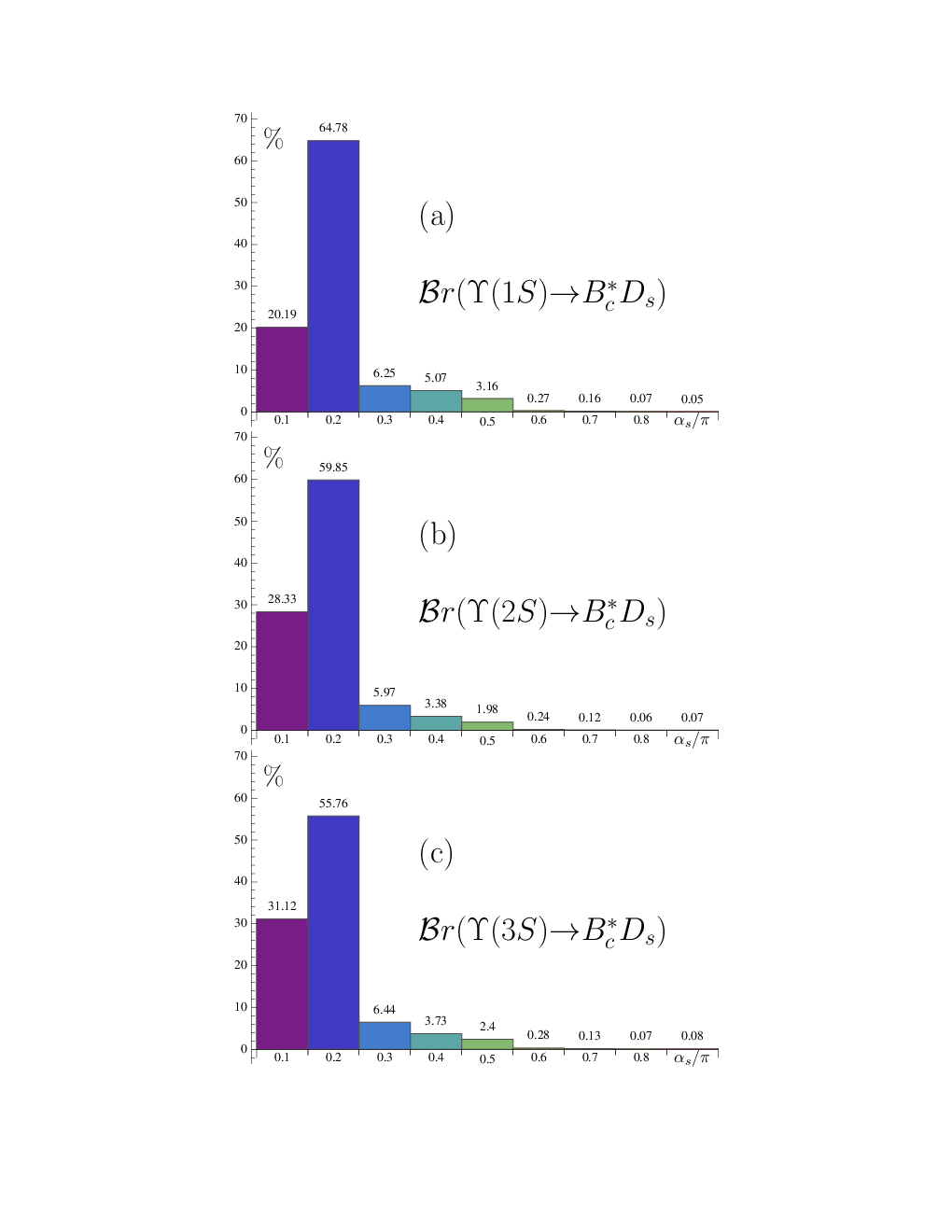
Figure 3: Contributions to branching ratio from different regions of αs/π{\alpha}_{s}/{\pi} (horizontal axis), where the numbers over histogram denote the percentage of the corresponding contributions.

(4) The momentum transition in Υ⁡(n​S){\Upsilon}(nS) →{\to} Bc∗​DB_{c}^{\ast}D decay may be not large enough, because of mBc∗m_{B_{c}^{\ast}} ++ mDm_{D} >> 8 GeV. It is natural to question the validity of perturbative calculation with pQCD approach. Therefore, it is very necessary to check what percentage of contributions comes from the perturbative region. In Fig.3, contributions to branching ratio from different regions of αs/π{\alpha}_{s}/{\pi} are plotted. It is clearly seen that more than 80% (90%) contributions come from αs/π{\alpha}_{s}/{\pi} ≤{\leq} 0.20.2 (0.30.3) regions, implying that pQCD approach is applicable to the concerned processes, and many combined factors (such as the choice of scale tt, Sudakov factor, wave function models, and so on) ensure a reliable perturbative calculation. Compared with the second bin contribution where αs/π{\alpha}_{s}/{\pi} == 0.20.2, the first bin contribution where αs/π{\alpha}_{s}/{\pi} == 0.10.1 is relatively small. One of crucial reasons might be that the absolute values of parameter a1a_{1} and coupling αs{\alpha}_{s} decrease along with the increase of renormalization scale.

(5) Besides the uncertainties listed in Table 2, decay constants fΥf_{\Upsilon} and fBc∗f_{B_{c}^{\ast}} (decay width ΓΥ{\Gamma}_{\Upsilon}) can bring about 7% (2%), 12% (8%), 16% (9%) uncertainties for Υ⁡(1​S){\Upsilon}(1S), Υ⁡(2​S){\Upsilon}(2S), Υ⁡(3​S){\Upsilon}(3S) decays, respectively, mainly from fΥ⁡(2​S,3​S)f_{{\Upsilon}(2S,3S)} and ΓΥ⁡(2​S,3​S){\Gamma}_{{\Upsilon}(2S,3S)}. These are at least two ways to reduce theoretical uncertainty. One way is to construct some relative ratios, for example, ℬ​r​(Υ⁡(n​S)→Bc∗​Dd)/ℬ​r​(Υ⁡(n​S)→Bc∗​Ds){\cal B}r({\Upsilon}(nS){\to}B_{c}^{\ast}D_{d})/{\cal B}r({\Upsilon}(nS){\to}B_{c}^{\ast}D_{s}) and ℬ​r​(Υ⁡(m​S)→Bc∗​D)/ℬ​r​(Υ⁡(n​S)→Bc∗​D){\cal B}r({\Upsilon}(mS){\to}B_{c}^{\ast}D)/{\cal B}r({\Upsilon}(nS){\to}B_{c}^{\ast}D). The other is to consider higher order corrections to HME, more realistic DAs models, and so on. Our results are just an order of magnitude estimation on branching ratio.

IV Summary

With anticipation of the potential prospects of Υ⁡(n​S){\Upsilon}(nS) physics at high-luminosity heavy-flavor factories, search for Υ⁡(n​S){\Upsilon}(nS) weak decay seems to be experimentally feasible. A theoretical study of Υ⁡(n​S){\Upsilon}(nS) weak decay is seasonable and necessary. In this paper, we investigated the bottom- and charm-changing Υ⁡(n​S){\Upsilon}(nS) →{\to} Bc∗​Ds,dB_{c}^{\ast}D_{s,d} decays with phenomenological pQCD approach. It is expected that branching ratio for Υ⁡(n​S){\Upsilon}(nS) →{\to} Bc∗​DsB_{c}^{\ast}D_{s} decay could be up to 𝒪⁡(10−10){\cal O}(10^{-10}), which might be measurable at the future LHC and SuperKEKB experiments.

Acknowledgments

The work is supported by the National Natural Science Foundation of China (Grant Nos. 11547014, 11475055, U1332103 and 11275057).

Appendix A Building blocks of decay amplitudes

For the sake of simplicity, we decompose the amplitude Eq.(55) into some building blocks 𝒜i,jk{\cal A}_{i,j}^{k}, where the subscript ii corresponds to the indices of Fig.2; the subscript jj == LL, NN, TT relates with different helicity amplitudes; the superscript kk refers to one of the three possible Dirac structures Γ1⊗Γ2{\Gamma}_{1}{\otimes}{\Gamma}_{2} of the four-quark operator (q¯1​Γ1​q2)​(q¯1​Γ2​q2)(\bar{q}_{1}{\Gamma}_{1}q_{2})(\bar{q}_{1}{\Gamma}_{2}q_{2}), namely kk == L​LLL for (V−A)⊗(V−A)(V-A){\otimes}(V-A), kk == L​RLR for (V−A)⊗(V+A)(V-A){\otimes}(V+A), and kk == S​PSP for −2(S−P)⊗(S+P)-2(S-P){\otimes}(S+P). The explicit expressions of 𝒜i,jk{\cal A}_{i,j}^{k} are written as follows.

𝒜a,LL​L=ℐa​ϕΥv​(x1)​{ϕBc∗v​(x2)​[m12​s−(4​m12​p2+m22​u)​x¯2]+ϕBc∗t​(x2)​m2​mb​u},{\cal A}_{a,L}^{LL}\ =\ {\cal I}_{a}\,{\phi}_{\Upsilon}^{v}(x_{1})\,\Big\{{\phi}_{B_{c}^{\ast}}^{v}(x_{2})\,\Big[m_{1}^{2}\,s-(4\,m_{1}^{2}\,p^{2}+m_{2}^{2}\,u)\,\bar{x}_{2}\Big]+{\phi}_{B_{c}^{\ast}}^{t}(x_{2})\,m_{2}\,m_{b}\,u\Big\}, (59)
𝒜a,NL​L=m1​ℐa​ϕΥV​(x1)​{ϕBc∗V​(x2)​m2​(u−s​x¯2)+ϕBc∗T​(x2)​mb​s},{\cal A}_{a,N}^{LL}\ =\ m_{1}\,{\cal I}_{a}\,{\phi}_{\Upsilon}^{V}(x_{1})\,\Big\{{\phi}_{B_{c}^{\ast}}^{V}(x_{2})\,m_{2}\,(u-s\,\bar{x}_{2})+{\phi}_{B_{c}^{\ast}}^{T}(x_{2})\,m_{b}\,s\Big\}, (60)
𝒜a,TL​L=−2​m1​ℐa​ϕΥV​(x1)​{ϕBc∗V​(x2)​m2​x2+ϕBc∗T​(x2)​mb},{\cal A}_{a,T}^{LL}\ =\ -2\,m_{1}\,{\cal I}_{a}\,{\phi}_{\Upsilon}^{V}(x_{1})\,\Big\{{\phi}_{B_{c}^{\ast}}^{V}(x_{2})\,m_{2}\,x_{2}+{\phi}_{B_{c}^{\ast}}^{T}(x_{2})\,m_{b}\Big\}, (61)
𝒜a,LS​P= 2​m3​ℐa​ϕΥv​(x1)​{ϕBc∗v​(x2)​mb​t+ϕBc∗t​(x2)​m2​(2​m12−t​x¯2)},{\cal A}_{a,L}^{SP}\ =\ 2\,m_{3}\,{\cal I}_{a}\,{\phi}_{\Upsilon}^{v}(x_{1})\,\Big\{{\phi}_{B_{c}^{\ast}}^{v}(x_{2})\,m_{b}\,t+{\phi}_{B_{c}^{\ast}}^{t}(x_{2})\,m_{2}\,(2\,m_{1}^{2}-t\,\bar{x}_{2})\Big\}, (62)
𝒜a,NS​P= 2​m1​m3​ℐa​ϕΥV​(x1)​{ϕBc∗V​(x2)​ 2​m2​mb+ϕBc∗T​(x2)​(t−2​m22​x¯2)},{\cal A}_{a,N}^{SP}\ =\ 2\,m_{1}\,m_{3}\,{\cal I}_{a}\,{\phi}_{\Upsilon}^{V}(x_{1})\,\Big\{{\phi}_{B_{c}^{\ast}}^{V}(x_{2})\,2\,m_{2}\,m_{b}+{\phi}_{B_{c}^{\ast}}^{T}(x_{2})\,(t-2\,m_{2}^{2}\,\bar{x}_{2})\Big\}, (63)
𝒜a,TS​P= 4​m1​m3​ℐa​ϕΥV​(x1)​ϕBc∗T​(x2),{\cal A}_{a,T}^{SP}\ =\ 4\,m_{1}\,m_{3}\,{\cal I}_{a}\,{\phi}_{\Upsilon}^{V}(x_{1})\,{\phi}_{B_{c}^{\ast}}^{T}(x_{2}), (64)
𝒜b,LL​L=ℐb​ϕBc∗v​(x2)​{ϕΥv​(x1)​[m22​u−m12​(s−4​p2)​x¯1]+ϕΥt​(x1)​m1​mc​s},{\cal A}_{b,L}^{LL}\ =\ {\cal I}_{b}\,{\phi}_{B_{c}^{\ast}}^{v}(x_{2})\,\Big\{{\phi}_{\Upsilon}^{v}(x_{1})\,\Big[m_{2}^{2}\,u-m_{1}^{2}\,(s-4\,p^{2})\,\bar{x}_{1}\Big]+{\phi}_{\Upsilon}^{t}(x_{1})\,m_{1}\,m_{c}\,s\Big\}, (65)
𝒜b,NL​L=m2​ℐb​ϕBc∗V​(x2)​{ϕΥV​(x1)​m1​(s−u​x¯1)+ϕΥT​(x1)​mc​u},{\cal A}_{b,N}^{LL}\ =\ m_{2}\,{\cal I}_{b}\,{\phi}_{B_{c}^{\ast}}^{V}(x_{2})\,\Big\{{\phi}_{\Upsilon}^{V}(x_{1})\,m_{1}\,(s-u\,\bar{x}_{1})+{\phi}_{\Upsilon}^{T}(x_{1})\,m_{c}\,u\Big\}, (66)
𝒜b,TL​L=−2​m2​ℐb​ϕBc∗V​(x2)​{ϕΥV​(x1)​m1​x1+ϕΥT​(x1)​mc},{\cal A}_{b,T}^{LL}\ =\ -2\,m_{2}\,{\cal I}_{b}\,{\phi}_{B_{c}^{\ast}}^{V}(x_{2})\,\Big\{{\phi}_{\Upsilon}^{V}(x_{1})\,m_{1}\,x_{1}+{\phi}_{\Upsilon}^{T}(x_{1})\,m_{c}\Big\}, (67)
𝒜b,LS​P= 2​m3​ℐb​ϕBc∗v​(x2)​{ϕΥv​(x1)​mc​t+ϕΥt​(x1)​m1​(2​m22−t​x¯1)},{\cal A}_{b,L}^{SP}\ =\ 2\,m_{3}\,{\cal I}_{b}\,{\phi}_{B_{c}^{\ast}}^{v}(x_{2})\,\Big\{{\phi}_{\Upsilon}^{v}(x_{1})\,m_{c}\,t+{\phi}_{\Upsilon}^{t}(x_{1})\,m_{1}\,(2\,m_{2}^{2}-t\,\bar{x}_{1})\Big\}, (68)
𝒜b,NS​P= 2​m2​m3​ℐb​ϕBc∗V​(x2)​{ϕΥV​(x1)​ 2​m1​mc+ϕΥT​(x1)​(t−2​m12​x¯1)},{\cal A}_{b,N}^{SP}\ =\ 2\,m_{2}\,m_{3}\,{\cal I}_{b}\,{\phi}_{B_{c}^{\ast}}^{V}(x_{2})\,\Big\{{\phi}_{\Upsilon}^{V}(x_{1})\,2\,m_{1}\,m_{c}+{\phi}_{\Upsilon}^{T}(x_{1})\,(t-2\,m_{1}^{2}\,\bar{x}_{1})\Big\}, (69)
𝒜b,TS​P= 4​m2​m3​ℐb​ϕΥT​(x1)​ϕBc∗V​(x2),{\cal A}_{b,T}^{SP}\ =\ 4\,m_{2}\,m_{3}\,{\cal I}_{b}\,{\phi}_{\Upsilon}^{T}(x_{1})\,{\phi}_{B_{c}^{\ast}}^{V}(x_{2}), (70)
𝒜c,LL​L\displaystyle{\cal A}_{c,L}^{LL} =\displaystyle= ℐcϕDa(x3){ϕΥv(x1)ϕBc∗v(x2) 4m12p2(x1−x¯3)\displaystyle{\cal I}_{c}\,{\phi}_{D}^{a}(x_{3})\,\Big\{{\phi}_{\Upsilon}^{v}(x_{1})\,{\phi}_{B_{c}^{\ast}}^{v}(x_{2})\,4\,m_{1}^{2}\,p^{2}\,(x_{1}-\bar{x}_{3}) (71)
+ϕΥt(x1)ϕBc∗t(x2)m1m2(ux1−sx2−2m32x¯3)},\displaystyle+{\phi}_{\Upsilon}^{t}(x_{1})\,{\phi}_{B_{c}^{\ast}}^{t}(x_{2})\,m_{1}\,m_{2}\,(u\,x_{1}-s\,x_{2}-2\,m_{3}^{2}\,\bar{x}_{3})\Big\},
𝒜c,NL​L=ℐc​ϕΥT​(x1)​ϕBc∗T​(x2)​ϕDa​(x3)​{m12​s​(x1−x¯3)+m22​u​(x¯3−x2)},{\cal A}_{c,N}^{LL}\ =\ {\cal I}_{c}\,{\phi}_{\Upsilon}^{T}(x_{1})\,{\phi}_{B_{c}^{\ast}}^{T}(x_{2})\,{\phi}_{D}^{a}(x_{3})\,\Big\{m_{1}^{2}\,s\,(x_{1}-\bar{x}_{3})+m_{2}^{2}\,u\,(\bar{x}_{3}-x_{2})\Big\}, (72)
𝒜c,TL​L= 2​ℐc​ϕΥT​(x1)​ϕBc∗T​(x2)​ϕDa​(x3)​{m12​(x¯3−x1)+m22​(x2−x¯3)},{\cal A}_{c,T}^{LL}\ =\ 2\,{\cal I}_{c}\,{\phi}_{\Upsilon}^{T}(x_{1})\,{\phi}_{B_{c}^{\ast}}^{T}(x_{2})\,{\phi}_{D}^{a}(x_{3})\,\Big\{m_{1}^{2}\,(\bar{x}_{3}-x_{1})+m_{2}^{2}\,(x_{2}-\bar{x}_{3})\Big\}, (73)
𝒜c,LS​P\displaystyle{\cal A}_{c,L}^{SP} =\displaystyle= ℐcϕDp(x3){ϕΥv(x1)ϕBc∗t(x2)m2m3(2m12x1−tx2−ux¯3)\displaystyle{\cal I}_{c}\,{\phi}_{D}^{p}(x_{3})\,\Big\{{\phi}_{\Upsilon}^{v}(x_{1})\,{\phi}_{B_{c}^{\ast}}^{t}(x_{2})\,m_{2}\,m_{3}\,(2\,m_{1}^{2}\,x_{1}-t\,x_{2}-u\,\bar{x}_{3}) (74)
+ϕΥt(x1)ϕBc∗v(x2)m1m3(tx1−2m22x2−sx¯3)},\displaystyle+{\phi}_{\Upsilon}^{t}(x_{1})\,{\phi}_{B_{c}^{\ast}}^{v}(x_{2})\,m_{1}\,m_{3}\,(t\,x_{1}-2\,m_{2}^{2}\,x_{2}-s\,\bar{x}_{3})\Big\},
𝒜c,NS​P\displaystyle{\cal A}_{c,N}^{SP} =\displaystyle= ℐcϕDp(x3){ϕΥV(x1)ϕBc∗T(x2)m1m3(tx1−2m22x2−sx¯3)\displaystyle{\cal I}_{c}\,{\phi}_{D}^{p}(x_{3})\,\Big\{{\phi}_{\Upsilon}^{V}(x_{1})\,{\phi}_{B_{c}^{\ast}}^{T}(x_{2})\,m_{1}\,m_{3}\,(t\,x_{1}-2\,m_{2}^{2}\,x_{2}-s\,\bar{x}_{3}) (75)
+ϕΥT(x1)ϕBc∗V(x2)m2m3(2m12x1−tx2−ux¯3)},\displaystyle+{\phi}_{\Upsilon}^{T}(x_{1})\,{\phi}_{B_{c}^{\ast}}^{V}(x_{2})\,m_{2}\,m_{3}\,(2\,m_{1}^{2}\,x_{1}-t\,x_{2}-u\,\bar{x}_{3})\Big\},
𝒜c,TS​P= 2​m3​ℐc​ϕDp​(x3)​{ϕΥV​(x1)​ϕBc∗T​(x2)​m1​(x1−x¯3)+ϕΥT​(x1)​ϕBc∗V​(x2)​m2​(x¯3−x2)},{\cal A}_{c,T}^{SP}\ =\ 2\,m_{3}\,{\cal I}_{c}\,{\phi}_{D}^{p}(x_{3})\,\Big\{{\phi}_{\Upsilon}^{V}(x_{1})\,{\phi}_{B_{c}^{\ast}}^{T}(x_{2})\,m_{1}\,(x_{1}-\bar{x}_{3})+{\phi}_{\Upsilon}^{T}(x_{1})\,{\phi}_{B_{c}^{\ast}}^{V}(x_{2})\,m_{2}\,(\bar{x}_{3}-x_{2})\Big\}, (76)
𝒜d,LL​L\displaystyle{\cal A}_{d,L}^{LL} =\displaystyle= ℐd{ϕΥt(x1)ϕBc∗t(x2)ϕDa(x3)m1m2(sx2+2m32x3−ux1)\displaystyle{\cal I}_{d}\,\Big\{{\phi}_{\Upsilon}^{t}(x_{1})\,{\phi}_{B_{c}^{\ast}}^{t}(x_{2})\,{\phi}_{D}^{a}(x_{3})\,m_{1}\,m_{2}\,(s\,x_{2}+2\,m_{3}^{2}\,x_{3}-u\,x_{1}) (77)
+\displaystyle+ ϕΥv(x1)ϕBc∗v(x2)[ϕDa(x3) 4m12p2(x3−x2)−ϕDp(x3)m3mct]},\displaystyle{\phi}_{\Upsilon}^{v}(x_{1}){\phi}_{B_{c}^{\ast}}^{v}(x_{2})\Big[{\phi}_{D}^{a}(x_{3})\,4\,m_{1}^{2}\,p^{2}\,(x_{3}-x_{2})-{\phi}_{D}^{p}(x_{3})\,m_{3}\,m_{c}\,t\Big]\Big\},
𝒜d,NL​L\displaystyle{\cal A}_{d,N}^{LL} =\displaystyle= ℐd{ϕΥT(x1)ϕBc∗T(x2)ϕDa(x3)[m12s(x3−x1)+m22u(x2−x3)]\displaystyle{\cal I}_{d}\,\Big\{{\phi}_{\Upsilon}^{T}(x_{1})\,{\phi}_{B_{c}^{\ast}}^{T}(x_{2})\,{\phi}_{D}^{a}(x_{3})\,\Big[m_{1}^{2}\,s\,(x_{3}-x_{1})+m_{2}^{2}\,u\,(x_{2}-x_{3})\Big] (78)
−\displaystyle- ϕΥV(x1)ϕBc∗V(x2)ϕDp(x3) 2m1m2m3mc},\displaystyle{\phi}_{\Upsilon}^{V}(x_{1})\,{\phi}_{B_{c}^{\ast}}^{V}(x_{2})\,{\phi}_{D}^{p}(x_{3})\,2\,m_{1}\,m_{2}\,m_{3}\,m_{c}\Big\},
𝒜d,TL​L= 2​ℐd​ϕΥT​(x1)​ϕBc∗T​(x2)​ϕDa​(x3)​{m12​(x1−x3)−m22​(x2−x3)},{\cal A}_{d,T}^{LL}\ =\ 2\,{\cal I}_{d}\,{\phi}_{\Upsilon}^{T}(x_{1})\,{\phi}_{B_{c}^{\ast}}^{T}(x_{2})\,{\phi}_{D}^{a}(x_{3})\,\Big\{m_{1}^{2}\,(x_{1}-x_{3})-m_{2}^{2}\,(x_{2}-x_{3})\Big\}, (79)
𝒜d,LS​P\displaystyle{\cal A}_{d,L}^{SP} =\displaystyle= ℐd{ϕΥv(x1)ϕBc∗t(x2)m2[ϕDp(x3)m3(tx2+ux3−2m12x1)−ϕDa(x3)mcu]\displaystyle{\cal I}_{d}\,\Big\{{\phi}_{\Upsilon}^{v}(x_{1})\,{\phi}_{B_{c}^{\ast}}^{t}(x_{2})\,m_{2}\,\Big[{\phi}_{D}^{p}(x_{3})\,m_{3}\,(t\,x_{2}+u\,x_{3}-2\,m_{1}^{2}\,x_{1})-{\phi}_{D}^{a}(x_{3})\,m_{c}\,u\Big] (80)
+\displaystyle+ ϕΥt(x1)ϕBc∗v(x2)m1[ϕDp(x3)m3(2m22x2+sx3−tx1)−ϕDa(x3)mcs]},\displaystyle{\phi}_{\Upsilon}^{t}(x_{1})\,{\phi}_{B_{c}^{\ast}}^{v}(x_{2})\,m_{1}\,\Big[{\phi}_{D}^{p}(x_{3})\,m_{3}\,(2\,m_{2}^{2}\,x_{2}+s\,x_{3}-t\,x_{1})-{\phi}_{D}^{a}(x_{3})\,m_{c}\,s\Big]\Big\},
𝒜d,NS​P\displaystyle{\cal A}_{d,N}^{SP} =\displaystyle= ℐd{ϕΥV(x1)ϕBc∗T(x2)m1[ϕDp(x3)m3(2m22x2+sx3−tx1)−ϕDa(x3)mcs]\displaystyle{\cal I}_{d}\,\Big\{{\phi}_{\Upsilon}^{V}(x_{1})\,{\phi}_{B_{c}^{\ast}}^{T}(x_{2})\,m_{1}\,\Big[{\phi}_{D}^{p}(x_{3})\,m_{3}\,(2\,m_{2}^{2}\,x_{2}+s\,x_{3}-t\,x_{1})-{\phi}_{D}^{a}(x_{3})\,m_{c}\,s\Big] (81)
+\displaystyle+ ϕΥT(x1)ϕBc∗V(x2)m2[ϕDp(x3)m3(tx2+ux3−2m12x1)−ϕDa(x3)mcu]},\displaystyle{\phi}_{\Upsilon}^{T}(x_{1})\,{\phi}_{B_{c}^{\ast}}^{V}(x_{2})\,m_{2}\,\Big[{\phi}_{D}^{p}(x_{3})\,m_{3}\,(t\,x_{2}+u\,x_{3}-2\,m_{1}^{2}\,x_{1})-{\phi}_{D}^{a}(x_{3})\,m_{c}\,u\Big]\Big\},
𝒜d,TS​P\displaystyle{\cal A}_{d,T}^{SP} =\displaystyle= 2ℐd{ϕΥV(x1)ϕBc∗T(x2)m1[ϕDp(x3)m3(x3−x1)−ϕDa(x3)mc]\displaystyle 2\,{\cal I}_{d}\,\Big\{{\phi}_{\Upsilon}^{V}(x_{1})\,{\phi}_{B_{c}^{\ast}}^{T}(x_{2})\,m_{1}\,\Big[{\phi}_{D}^{p}(x_{3})\,m_{3}\,(x_{3}-x_{1})-{\phi}_{D}^{a}(x_{3})\,m_{c}\Big] (82)
+\displaystyle+ ϕΥT(x1)ϕBc∗V(x2)m2[ϕDa(x3)mc+ϕDp(x3)m3(x2−x3)]},\displaystyle{\phi}_{\Upsilon}^{T}(x_{1})\,{\phi}_{B_{c}^{\ast}}^{V}(x_{2})\,m_{2}\,\Big[{\phi}_{D}^{a}(x_{3})\,m_{c}+{\phi}_{D}^{p}(x_{3})\,{m}_{3}\,(x_{2}-x_{3})\Big]\Big\},
𝒜e,LL​L\displaystyle{\cal A}_{e,L}^{LL} =\displaystyle= ℐe{ϕBc∗v(x2)ϕDa(x3)[ϕΥv(x1) 4m12p2(x1−x¯3)−ϕΥt(x1)m1mbs]\displaystyle{\cal I}_{e}\,\Big\{{\phi}_{B_{c}^{\ast}}^{v}(x_{2})\,{\phi}_{D}^{a}(x_{3})\,\Big[{\phi}_{\Upsilon}^{v}(x_{1})\,4\,m_{1}^{2}\,p^{2}\,(x_{1}-\bar{x}_{3})-{\phi}_{\Upsilon}^{t}(x_{1})\,m_{1}\,m_{b}\,s\Big] (83)
+\displaystyle+ ϕΥv(x1)ϕBc∗t(x2)ϕDp(x3)m2m3(2m12x1−tx2−ux¯3)},\displaystyle{\phi}_{\Upsilon}^{v}(x_{1})\,{\phi}_{B_{c}^{\ast}}^{t}(x_{2})\,{\phi}_{D}^{p}(x_{3})\,m_{2}\,m_{3}\,(2\,m_{1}^{2}\,x_{1}-t\,x_{2}-u\,\bar{x}_{3})\Big\},
𝒜e,NL​L\displaystyle{\cal A}_{e,N}^{LL} =\displaystyle= ℐe{ϕΥV(x1)ϕBc∗T(x2)ϕDp(x3)m1m3(tx1−2m22x2−sx¯3)\displaystyle{\cal I}_{e}\,\Big\{{\phi}_{\Upsilon}^{V}(x_{1}){\phi}_{B_{c}^{\ast}}^{T}(x_{2})\,{\phi}_{D}^{p}(x_{3})\,m_{1}\,m_{3}\,(t\,x_{1}-2\,m_{2}^{2}\,x_{2}-s\,\bar{x}_{3}) (84)
−\displaystyle- ϕΥT(x1)ϕBc∗V(x2)ϕDa(x3)m2mbu},\displaystyle{\phi}_{\Upsilon}^{T}(x_{1})\,{\phi}_{B_{c}^{\ast}}^{V}(x_{2})\,{\phi}_{D}^{a}(x_{3})\,m_{2}\,m_{b}\,u\Big\},
𝒜e,TL​L= 2​ℐe​{ϕΥV​(x1)​ϕBc∗T​(x2)​ϕDp​(x3)​m1​m3​(x1−x¯3)−ϕΥT​(x1)​ϕBc∗V​(x2)​ϕDa​(x3)​m2​mb},{\cal A}_{e,T}^{LL}\ =\ 2\,{\cal I}_{e}\,\Big\{{\phi}_{\Upsilon}^{V}(x_{1}){\phi}_{B_{c}^{\ast}}^{T}(x_{2})\,{\phi}_{D}^{p}(x_{3})\,m_{1}\,m_{3}\,(x_{1}-\bar{x}_{3})-{\phi}_{\Upsilon}^{T}(x_{1})\,{\phi}_{B_{c}^{\ast}}^{V}(x_{2})\,{\phi}_{D}^{a}(x_{3})\,m_{2}\,m_{b}\Big\}, (85)
𝒜e,LL​R\displaystyle{\cal A}_{e,L}^{LR} =\displaystyle= ℐe{ϕBc∗v(x2)ϕDa(x3)[ϕΥv(x1)t(sx2+2m32x¯3−ux1)+ϕΥt(x1)m1mbs]\displaystyle{\cal I}_{e}\,\Big\{{\phi}_{B_{c}^{\ast}}^{v}(x_{2})\,{\phi}_{D}^{a}(x_{3})\,\Big[{\phi}_{\Upsilon}^{v}(x_{1})\,t\,(s\,x_{2}+2\,m_{3}^{2}\,\bar{x}_{3}-u\,x_{1})+{\phi}_{\Upsilon}^{t}(x_{1})\,m_{1}\,m_{b}\,s\Big] (86)
+\displaystyle+ ϕBc∗t(x2)ϕDp(x3)m2m3[ϕΥv(x1)(tx2+ux¯3−2m12x1)+ϕΥt(x1) 4m1mb]},\displaystyle{\phi}_{B_{c}^{\ast}}^{t}(x_{2})\,{\phi}_{D}^{p}(x_{3})\,m_{2}\,m_{3}\,\Big[{\phi}_{\Upsilon}^{v}(x_{1})\,(t\,x_{2}+u\,\bar{x}_{3}-2\,m_{1}^{2}\,x_{1})+{\phi}_{\Upsilon}^{t}(x_{1})\,4\,m_{1}\,m_{b}\Big]\Big\},
𝒜e,NL​R\displaystyle{\cal A}_{e,N}^{LR} =\displaystyle= ℐe{ϕBc∗V(x2)ϕDa(x3)m2[ϕΥV(x1) 2m1(sx2+2m32x¯3−ux1)+ϕΥT(x1)mbu]\displaystyle{\cal I}_{e}\,\Big\{{\phi}_{B_{c}^{\ast}}^{V}(x_{2})\,{\phi}_{D}^{a}(x_{3})\,m_{2}\,\Big[{\phi}_{\Upsilon}^{V}(x_{1})\,2\,m_{1}\,(s\,x_{2}+2\,m_{3}^{2}\,\bar{x}_{3}-u\,x_{1})+{\phi}_{\Upsilon}^{T}(x_{1})\,m_{b}\,u\Big] (87)
+\displaystyle+ ϕBc∗T(x2)ϕDp(x3)m3[ϕΥV(x1)m1(2m22x2+sx¯3−tx1)+ϕΥT(x1) 2mbt]},\displaystyle{\phi}_{B_{c}^{\ast}}^{T}(x_{2})\,{\phi}_{D}^{p}(x_{3})\,m_{3}\,\Big[{\phi}_{\Upsilon}^{V}(x_{1})\,m_{1}\,(2\,m_{2}^{2}\,x_{2}+s\,\bar{x}_{3}-t\,x_{1})+{\phi}_{\Upsilon}^{T}(x_{1})\,2\,m_{b}\,t\Big]\Big\},
𝒜e,TL​R\displaystyle{\cal A}_{e,T}^{LR} =\displaystyle= 2ℐe{ϕBc∗T(x2)ϕDp(x3)m3[ϕΥV(x1)m1(x¯3−x1)+ϕΥT(x1) 2mb]\displaystyle 2\,{\cal I}_{e}\,\Big\{{\phi}_{B_{c}^{\ast}}^{T}(x_{2})\,{\phi}_{D}^{p}(x_{3})\,m_{3}\,\Big[{\phi}_{\Upsilon}^{V}(x_{1})\,m_{1}\,(\bar{x}_{3}-x_{1})+{\phi}_{\Upsilon}^{T}(x_{1})\,2\,m_{b}\Big] (88)
−\displaystyle- ϕΥT(x1)ϕBc∗V(x2)ϕDa(x3)m2mb},\displaystyle{\phi}_{\Upsilon}^{T}(x_{1})\,{\phi}_{B_{c}^{\ast}}^{V}(x_{2})\,{\phi}_{D}^{a}(x_{3})\,m_{2}\,m_{b}\Big\},
𝒜e,LS​P\displaystyle{\cal A}_{e,L}^{SP} =\displaystyle= ℐe{ϕBc∗t(x2)ϕDa(x3)m2[ϕΥv(x1)mbu+ϕΥt(x1)m1(sx2+2m32x¯3−ux1)]\displaystyle{\cal I}_{e}\,\Big\{{\phi}_{B_{c}^{\ast}}^{t}(x_{2})\,{\phi}_{D}^{a}(x_{3})\,m_{2}\,\Big[{\phi}_{\Upsilon}^{v}(x_{1})\,m_{b}\,u+{\phi}_{\Upsilon}^{t}(x_{1})\,m_{1}\,(s\,x_{2}+2\,m_{3}^{2}\,\bar{x}_{3}-u\,x_{1})\Big] (89)
+\displaystyle+ ϕBc∗v(x2)ϕDp(x3)m3[ϕΥv(x1)mbt+ϕΥt(x1)m1(2m22x2+sx¯3−tx1)]},\displaystyle{\phi}_{B_{c}^{\ast}}^{v}(x_{2})\,{\phi}_{D}^{p}(x_{3})\,m_{3}\,\Big[{\phi}_{\Upsilon}^{v}(x_{1})\,m_{b}\,t+{\phi}_{\Upsilon}^{t}(x_{1})\,m_{1}\,(2\,m_{2}^{2}\,x_{2}+s\,\bar{x}_{3}-t\,x_{1})\Big]\Big\},
𝒜e,NS​P\displaystyle{\cal A}_{e,N}^{SP} =\displaystyle= ℐe{ϕBc∗T(x2)ϕDa(x3)[ϕΥV(x1)m1mbs+ϕΥT(x1){m12s(x¯3−x1)+m22u(x2−x¯3)}]\displaystyle{\cal I}_{e}\,\Big\{{\phi}_{B_{c}^{\ast}}^{T}(x_{2})\,{\phi}_{D}^{a}(x_{3})\,\Big[{\phi}_{\Upsilon}^{V}(x_{1})\,m_{1}\,m_{b}\,s+{\phi}_{\Upsilon}^{T}(x_{1})\,\{m_{1}^{2}\,s\,(\bar{x}_{3}-x_{1})+m_{2}^{2}\,u\,(x_{2}-\bar{x}_{3})\}\Big] (90)
+\displaystyle+ ϕBc∗V(x2)ϕDp(x3)m2m3[ϕΥV(x1) 2m1mb+ϕΥT(x1)(tx2+ux¯3−2m12x1)]},\displaystyle{\phi}_{B_{c}^{\ast}}^{V}(x_{2})\,{\phi}_{D}^{p}(x_{3})\,m_{2}\,m_{3}\,\Big[{\phi}_{\Upsilon}^{V}(x_{1})\,2\,m_{1}\,m_{b}+{\phi}_{\Upsilon}^{T}(x_{1})\,(t\,x_{2}+u\,\bar{x}_{3}-2\,m_{1}^{2}\,x_{1})\Big]\Big\},
𝒜e,TS​P\displaystyle{\cal A}_{e,T}^{SP} =\displaystyle= 2ℐe{ϕBc∗T(x2)ϕDa(x3)[ϕΥV(x1)m1mb+ϕΥT(x1){m12(x¯3−x1)+m22(x2−x¯3)}]\displaystyle 2\,{\cal I}_{e}\,\Big\{{\phi}_{B_{c}^{\ast}}^{T}(x_{2})\,{\phi}_{D}^{a}(x_{3})\,\Big[{\phi}_{\Upsilon}^{V}(x_{1})\,m_{1}\,m_{b}+{\phi}_{\Upsilon}^{T}(x_{1})\,\{m_{1}^{2}\,(\bar{x}_{3}-x_{1})+m_{2}^{2}\,(x_{2}-\bar{x}_{3})\}\Big] (91)
+\displaystyle+ ϕΥT(x1)ϕBc∗V(x2)ϕDp(x3)m2m3(x¯3−x2)]},\displaystyle{\phi}_{\Upsilon}^{T}(x_{1})\,{\phi}_{B_{c}^{\ast}}^{V}(x_{2})\,{\phi}_{D}^{p}(x_{3})\,m_{2}\,m_{3}\,(\bar{x}_{3}-x_{2})\Big]\Big\},
𝒜f,LL​L\displaystyle{\cal A}_{f,L}^{LL} =\displaystyle= ℐf{ϕBc∗v(x2)ϕDa(x3)[ϕΥv(x1)t(ux¯1−sx2−2m32x¯3)−ϕΥt(x1)m1mbs]\displaystyle{\cal I}_{f}\,\Big\{{\phi}_{B_{c}^{\ast}}^{v}(x_{2})\,{\phi}_{D}^{a}(x_{3})\,\Big[{\phi}_{\Upsilon}^{v}(x_{1})\,t\,(u\,\bar{x}_{1}-s\,x_{2}-2\,m_{3}^{2}\,\bar{x}_{3})-{\phi}_{\Upsilon}^{t}(x_{1})\,m_{1}\,m_{b}\,s\Big] (92)
+\displaystyle+ ϕBc∗t(x2)ϕDp(x3)m2m3[ϕΥv(x1)(2m12x¯1−tx2−ux¯3)−ϕΥt(x1) 4m1mb]},\displaystyle{\phi}_{B_{c}^{\ast}}^{t}(x_{2})\,{\phi}_{D}^{p}(x_{3})\,m_{2}\,m_{3}\,\Big[{\phi}_{\Upsilon}^{v}(x_{1})\,(2\,m_{1}^{2}\,\bar{x}_{1}-t\,x_{2}-u\,\bar{x}_{3})-{\phi}_{\Upsilon}^{t}(x_{1})\,4\,m_{1}\,m_{b}\Big]\Big\},
𝒜f,NL​L\displaystyle{\cal A}_{f,N}^{LL} =\displaystyle= ℐf{ϕBc∗V(x2)ϕDa(x3)m2[ϕΥV(x1) 2m1(ux¯1−sx2−2m32x¯3)−ϕΥT(x1)mbu]\displaystyle{\cal I}_{f}\,\Big\{{\phi}_{B_{c}^{\ast}}^{V}(x_{2})\,{\phi}_{D}^{a}(x_{3})\,m_{2}\,\Big[{\phi}_{\Upsilon}^{V}(x_{1})\,2\,m_{1}\,(u\,\bar{x}_{1}-s\,x_{2}-2\,m_{3}^{2}\,\bar{x}_{3})-{\phi}_{\Upsilon}^{T}(x_{1})\,m_{b}\,u\Big] (93)
+\displaystyle+ ϕBc∗T(x2)ϕDp(x3)m3[ϕΥV(x1)m1(tx¯1−2m22x2−sx¯3)−ϕΥT(x1) 2mbt]},\displaystyle{\phi}_{B_{c}^{\ast}}^{T}(x_{2})\,{\phi}_{D}^{p}(x_{3})\,m_{3}\,\Big[{\phi}_{\Upsilon}^{V}(x_{1})\,m_{1}\,(t\,\bar{x}_{1}-2\,m_{2}^{2}\,x_{2}-s\,\bar{x}_{3})-{\phi}_{\Upsilon}^{T}(x_{1})\,2\,m_{b}\,t\Big]\Big\},
𝒜f,TL​L\displaystyle{\cal A}_{f,T}^{LL} =\displaystyle= 2ℐf{ϕBc∗T(x2)ϕDp(x3)m3[ϕΥV(x1)m1(x¯1−x¯3)−ϕΥT(x1) 2mb]\displaystyle 2\,{\cal I}_{f}\,\Big\{{\phi}_{B_{c}^{\ast}}^{T}(x_{2})\,{\phi}_{D}^{p}(x_{3})\,m_{3}\,\Big[{\phi}_{\Upsilon}^{V}(x_{1})\,m_{1}\,(\bar{x}_{1}-\bar{x}_{3})-{\phi}_{\Upsilon}^{T}(x_{1})\,2\,m_{b}\Big] (94)
+\displaystyle+ ϕΥT(x1)ϕBc∗V(x2)ϕDa(x3)m2mb},\displaystyle{\phi}_{\Upsilon}^{T}(x_{1})\,{\phi}_{B_{c}^{\ast}}^{V}(x_{2})\,{\phi}_{D}^{a}(x_{3})\,m_{2}\,m_{b}\Big\},
𝒜f,LL​R\displaystyle{\cal A}_{f,L}^{LR} =\displaystyle= ℐf{ϕBc∗v(x2)ϕDa(x3)[ϕΥv(x1) 4m12p2(x¯3−x¯1)+ϕΥt(x1)m1mbs]\displaystyle{\cal I}_{f}\,\Big\{{\phi}_{B_{c}^{\ast}}^{v}(x_{2})\,{\phi}_{D}^{a}(x_{3})\,\Big[{\phi}_{\Upsilon}^{v}(x_{1})\,4\,m_{1}^{2}\,p^{2}\,(\bar{x}_{3}-\bar{x}_{1})+{\phi}_{\Upsilon}^{t}(x_{1})\,m_{1}\,m_{b}\,s\Big] (95)
+\displaystyle+ ϕΥv(x1)ϕBc∗t(x2)ϕDp(x3)m2m3(tx2+ux¯3−2m12x¯1)},\displaystyle{\phi}_{\Upsilon}^{v}(x_{1})\,{\phi}_{B_{c}^{\ast}}^{t}(x_{2})\,{\phi}_{D}^{p}(x_{3})\,m_{2}\,m_{3}\,(t\,x_{2}+u\,\bar{x}_{3}-2\,m_{1}^{2}\,\bar{x}_{1})\Big\},
𝒜f,NL​R\displaystyle{\cal A}_{f,N}^{LR} =\displaystyle= ℐf{ϕΥV(x1)ϕBc∗T(x2)ϕDp(x3)m1m3(2m22x2+sx¯3−tx¯1)\displaystyle{\cal I}_{f}\,\Big\{{\phi}_{\Upsilon}^{V}(x_{1})\,{\phi}_{B_{c}^{\ast}}^{T}(x_{2})\,{\phi}_{D}^{p}(x_{3})\,m_{1}\,m_{3}\,(2\,m_{2}^{2}\,x_{2}+s\,\bar{x}_{3}-t\,\bar{x}_{1}) (96)
+\displaystyle+ ϕΥT(x1)ϕBc∗V(x2)ϕDa(x3)m2mbu},\displaystyle{\phi}_{\Upsilon}^{T}(x_{1})\,{\phi}_{B_{c}^{\ast}}^{V}(x_{2})\,{\phi}_{D}^{a}(x_{3})\,m_{2}\,m_{b}\,u\Big\},
𝒜f,TL​R= 2​ℐf​{ϕΥT​(x1)​ϕBc∗V​(x2)​ϕDa​(x3)​m2​mb+ϕΥV​(x1)​ϕBc∗T​(x2)​ϕDp​(x3)​m1​m3​(x¯3−x¯1)},{\cal A}_{f,T}^{LR}\ =\ 2\,{\cal I}_{f}\,\Big\{{\phi}_{\Upsilon}^{T}(x_{1})\,{\phi}_{B_{c}^{\ast}}^{V}(x_{2})\,{\phi}_{D}^{a}(x_{3})\,m_{2}\,m_{b}+{\phi}_{\Upsilon}^{V}(x_{1})\,{\phi}_{B_{c}^{\ast}}^{T}(x_{2})\,{\phi}_{D}^{p}(x_{3})\,m_{1}\,m_{3}\,(\bar{x}_{3}-\bar{x}_{1})\Big\}, (97)
𝒜f,LS​P\displaystyle{\cal A}_{f,L}^{SP} =\displaystyle= ℐf{ϕBc∗t(x2)ϕDa(x3)m2[ϕΥv(x1)mbu+ϕΥt(x1)m1(sx2+2m32x¯3−ux¯1)]\displaystyle{\cal I}_{f}\,\Big\{{\phi}_{B_{c}^{\ast}}^{t}(x_{2})\,{\phi}_{D}^{a}(x_{3})\,m_{2}\,\Big[{\phi}_{\Upsilon}^{v}(x_{1})\,m_{b}\,u+{\phi}_{\Upsilon}^{t}(x_{1})\,m_{1}\,(s\,x_{2}+2\,m_{3}^{2}\,\bar{x}_{3}-u\,\bar{x}_{1})\Big] (98)
+\displaystyle+ ϕBc∗v(x2)ϕDp(x3)m3[ϕΥv(x1)mbt+ϕΥt(x1)m1(2m22x2+sx¯3−tx¯1)]},\displaystyle{\phi}_{B_{c}^{\ast}}^{v}(x_{2})\,{\phi}_{D}^{p}(x_{3})\,m_{3}\,\Big[{\phi}_{\Upsilon}^{v}(x_{1})\,m_{b}\,t+{\phi}_{\Upsilon}^{t}(x_{1})\,m_{1}\,(2\,m_{2}^{2}\,x_{2}+s\,\bar{x}_{3}-t\,\bar{x}_{1})\Big]\Big\},
𝒜f,NS​P\displaystyle{\cal A}_{f,N}^{SP} =\displaystyle= ℐf{ϕBc∗T(x2)ϕDa(x3)[ϕΥV(x1)m1mbs+ϕΥT(x1){m12s(x¯3−x¯1)+m22u(x2−x¯3)}]\displaystyle{\cal I}_{f}\,\Big\{{\phi}_{B_{c}^{\ast}}^{T}(x_{2})\,{\phi}_{D}^{a}(x_{3})\,\Big[{\phi}_{\Upsilon}^{V}(x_{1})\,m_{1}\,m_{b}\,s+{\phi}_{\Upsilon}^{T}(x_{1})\,\{m_{1}^{2}\,s\,(\bar{x}_{3}-\bar{x}_{1})+m_{2}^{2}\,u\,(x_{2}-\bar{x}_{3})\}\Big] (99)
+\displaystyle+ ϕBc∗V(x2)ϕDp(x3)m2m3[ϕΥV(x1) 2m1mb+ϕΥT(x1)(tx2+ux¯3−2m12x¯1)]},\displaystyle{\phi}_{B_{c}^{\ast}}^{V}(x_{2})\,{\phi}_{D}^{p}(x_{3})\,m_{2}\,m_{3}\,\Big[{\phi}_{\Upsilon}^{V}(x_{1})\,2\,m_{1}\,m_{b}+{\phi}_{\Upsilon}^{T}(x_{1})\,(t\,x_{2}+u\,\bar{x}_{3}-2\,m_{1}^{2}\,\bar{x}_{1})\Big]\Big\},
𝒜f,TS​P\displaystyle{\cal A}_{f,T}^{SP} =\displaystyle= 2ℐf{ϕBc∗T(x2)ϕDa(x3)[ϕΥV(x1)m1mb+ϕΥT(x1){m12(x¯3−x¯1)+m22(x2−x¯3)}]\displaystyle 2\,{\cal I}_{f}\,\Big\{{\phi}_{B_{c}^{\ast}}^{T}(x_{2})\,{\phi}_{D}^{a}(x_{3})\,\Big[{\phi}_{\Upsilon}^{V}(x_{1})\,m_{1}\,m_{b}+{\phi}_{\Upsilon}^{T}(x_{1})\,\{m_{1}^{2}\,(\bar{x}_{3}-\bar{x}_{1})+m_{2}^{2}\,(x_{2}-\bar{x}_{3})\}\Big] (100)
+\displaystyle+ ϕΥT(x1)ϕBc∗V(x2)ϕDp(x3)m2m3(x¯3−x2)},\displaystyle{\phi}_{\Upsilon}^{T}(x_{1})\,{\phi}_{B_{c}^{\ast}}^{V}(x_{2})\,{\phi}_{D}^{p}(x_{3})\,m_{2}\,m_{3}\,(\bar{x}_{3}-x_{2})\Big\},
𝒜g,LL​L,L​R=ℐg​{ϕBc∗v​(x2)​ϕDa​(x3)​(m32​t​x¯2+m12​s​x2)+ϕBc∗t​(x2)​ϕDp​(x3)​ 2​m2​m3​(u+t​x2)},{\cal A}_{g,L}^{LL,LR}={\cal I}_{g}\,\Big\{{\phi}_{B_{c}^{\ast}}^{v}(x_{2})\,{\phi}_{D}^{a}(x_{3})\,(m_{3}^{2}\,t\,\bar{x}_{2}+m_{1}^{2}\,s\,x_{2})+{\phi}_{B_{c}^{\ast}}^{t}(x_{2})\,{\phi}_{D}^{p}(x_{3})\,2\,m_{2}\,m_{3}\,(u+t\,x_{2})\Big\}, (101)
𝒜g,NL​L,L​R=m1​ℐg​{ϕBc∗V​(x2)​ϕDa​(x3)​m2​(2​m32+s​x2)+ϕBc∗T​(x2)​ϕDp​(x3)​ 2​m3​(s+2​m22​x2)},\!{\cal A}_{g,N}^{LL,LR}=m_{1}\,{\cal I}_{g}\,\Big\{{\phi}_{B_{c}^{\ast}}^{V}(x_{2})\,{\phi}_{D}^{a}(x_{3})\,m_{2}\,(2\,m_{3}^{2}+s\,x_{2})+{\phi}_{B_{c}^{\ast}}^{T}(x_{2})\,{\phi}_{D}^{p}(x_{3})\,2\,m_{3}\,(s+2\,m_{2}^{2}\,x_{2})\Big\}, (102)
𝒜g,TL​L,L​R=2​m1​ℐg​{ϕBc∗T​(x2)​ϕDp​(x3)​ 2​m3−ϕBc∗V​(x2)​ϕDqa​(x3)​m2​x2},{\cal A}_{g,T}^{LL,LR}=2\,m_{1}\,{\cal I}_{g}\,\Big\{{\phi}_{B_{c}^{\ast}}^{T}(x_{2})\,{\phi}_{D}^{p}(x_{3})\,2\,m_{3}-{\phi}_{B_{c}^{\ast}}^{V}(x_{2})\,{\phi}_{D_{q}}^{a}(x_{3})\,m_{2}\,x_{2}\Big\}, (103)
𝒜h,LL​L,L​R=ℐh​ϕBc∗v​(x2)​{ϕDa​(x3)​(m22​u​x3+m12​s​x¯3)−ϕDp​(x3)​m3​mb​t},{\cal A}_{h,L}^{LL,LR}\,=\,{\cal I}_{h}\,{\phi}_{B_{c}^{\ast}}^{v}(x_{2})\,\Big\{{\phi}_{D}^{a}(x_{3})\,(m_{2}^{2}\,u\,x_{3}+m_{1}^{2}\,s\,\bar{x}_{3})-{\phi}_{D}^{p}(x_{3})\,m_{3}\,m_{b}\,t\Big\}, (104)
𝒜h,NL​L,L​R=m1​m2​ℐh​ϕBc∗V​(x2)​{ϕDa​(x3)​(s+2​m32​x¯3)−ϕDp​(x3)​ 2​m3​mb},{\cal A}_{h,N}^{LL,LR}\,=\,m_{1}\,m_{2}\,{\cal I}_{h}\,{\phi}_{B_{c}^{\ast}}^{V}(x_{2})\,\Big\{{\phi}_{D}^{a}(x_{3})\,(s+2\,m_{3}^{2}\,\bar{x}_{3})-{\phi}_{D}^{p}(x_{3})\,2\,m_{3}\,m_{b}\Big\}, (105)
𝒜h,TL​L,L​R= 2​m1​m2​ℐh​ϕBc∗V​(x2)​ϕDa​(x3),{\cal A}_{h,T}^{LL,LR}\,=\,2\,m_{1}\,m_{2}\,{\cal I}_{h}\,{\phi}_{B_{c}^{\ast}}^{V}(x_{2})\,{\phi}_{D}^{a}(x_{3}), (106)
ℐa=∫01d​x1​∫01d​x2​∫0∞b1​d​b1​∫0∞b2​d​b2​Ha​(αe,βa,b1,b2)​Ea​(ta)​αs​(ta),{\cal I}_{a}\ =\ {\int}_{0}^{1}dx_{1}{\int}_{0}^{1}dx_{2}{\int}_{0}^{\infty}b_{1}db_{1}{\int}_{0}^{\infty}b_{2}db_{2}\,H_{a}({\alpha}_{e},{\beta}_{a},b_{1},b_{2})\,E_{a}(t_{a})\,{\alpha}_{s}(t_{a}), (107)
ℐb=∫01d​x1​∫01d​x2​∫0∞b1​d​b1​∫0∞b2​d​b2​Hb​(αe,βb,b1,b2)​Eb​(tb)​αs​(tb),{\cal I}_{b}\ =\ {\int}_{0}^{1}dx_{1}{\int}_{0}^{1}dx_{2}{\int}_{0}^{\infty}b_{1}db_{1}{\int}_{0}^{\infty}b_{2}db_{2}\,H_{b}({\alpha}_{e},{\beta}_{b},b_{1},b_{2})\,E_{b}(t_{b})\,{\alpha}_{s}(t_{b}), (108)
ℐc\displaystyle{\cal I}_{c} =\displaystyle= 1Nc​∫01d​x1​∫01d​x2​∫01d​x3​∫0∞d​b1​∫0∞b2​d​b2​∫0∞b3​d​b3\displaystyle\frac{1}{N_{c}}{\int}_{0}^{1}dx_{1}{\int}_{0}^{1}dx_{2}{\int}_{0}^{1}dx_{3}{\int}_{0}^{\infty}db_{1}{\int}_{0}^{\infty}b_{2}db_{2}{\int}_{0}^{\infty}b_{3}db_{3} (109)
×\displaystyle{\times} Hc​(αe,βc,b2,b3)​Ec​(tc)​αs​(tc)​δ​(b1−b2),\displaystyle H_{c}({\alpha}_{e},{\beta}_{c},b_{2},b_{3})\,E_{c}(t_{c})\,{\alpha}_{s}(t_{c})\,{\delta}(b_{1}-b_{2})\,,
ℐd\displaystyle{\cal I}_{d} =\displaystyle= 1Nc​∫01d​x1​∫01d​x2​∫01d​x3​∫0∞d​b1​∫0∞b2​d​b2​∫0∞b3​d​b3\displaystyle\frac{1}{N_{c}}{\int}_{0}^{1}dx_{1}{\int}_{0}^{1}dx_{2}{\int}_{0}^{1}dx_{3}{\int}_{0}^{\infty}db_{1}{\int}_{0}^{\infty}b_{2}db_{2}{\int}_{0}^{\infty}b_{3}db_{3} (110)
×\displaystyle{\times} Hd​(αe,βd,b2,b3)​Ed​(td)​αs​(td)​δ​(b1−b2),\displaystyle H_{d}({\alpha}_{e},{\beta}_{d},b_{2},b_{3})\,E_{d}(t_{d})\,{\alpha}_{s}(t_{d})\,{\delta}(b_{1}-b_{2})\,,
ℐe\displaystyle{\cal I}_{e} =\displaystyle= 1Nc​∫01d​x1​∫01d​x2​∫01d​x3​∫0∞b1​d​b1​∫0∞b2​d​b2​∫0∞d​b3\displaystyle\frac{1}{N_{c}}{\int}_{0}^{1}dx_{1}{\int}_{0}^{1}dx_{2}{\int}_{0}^{1}dx_{3}{\int}_{0}^{\infty}b_{1}db_{1}{\int}_{0}^{\infty}b_{2}db_{2}{\int}_{0}^{\infty}db_{3} (111)
×\displaystyle{\times} He​(αa,βe,b1,b2)​Ee​(te)​αs​(te)​δ​(b2−b3),\displaystyle H_{e}({\alpha}_{a},{\beta}_{e},b_{1},b_{2})\,E_{e}(t_{e})\,{\alpha}_{s}(t_{e})\,{\delta}(b_{2}-b_{3}),
ℐf\displaystyle{\cal I}_{f} =\displaystyle= 1Nc​∫01d​x1​∫01d​x2​∫01d​x3​∫0∞b1​d​b1​∫0∞b2​d​b2​∫0∞d​b3\displaystyle\frac{1}{N_{c}}{\int}_{0}^{1}dx_{1}{\int}_{0}^{1}dx_{2}{\int}_{0}^{1}dx_{3}{\int}_{0}^{\infty}b_{1}db_{1}{\int}_{0}^{\infty}b_{2}db_{2}{\int}_{0}^{\infty}db_{3} (112)
×\displaystyle{\times} Hf​(αa,βf,b1,b2)​Ef​(tf)​αs​(tf)​δ​(b2−b3),\displaystyle H_{f}({\alpha}_{a},{\beta}_{f},b_{1},b_{2})\,E_{f}(t_{f})\,{\alpha}_{s}(t_{f})\,{\delta}(b_{2}-b_{3}),
ℐg=∫01d​x2​∫01d​x3​∫0∞b2​d​b2​∫0∞b3​d​b3​Hg​(αa,βg,b2,b3)​Eg​(tg)​αs​(tg),{\cal I}_{g}\ =\ {\int}_{0}^{1}dx_{2}{\int}_{0}^{1}dx_{3}{\int}_{0}^{\infty}b_{2}db_{2}{\int}_{0}^{\infty}b_{3}db_{3}\,H_{g}({\alpha}_{a},{\beta}_{g},b_{2},b_{3})\,E_{g}(t_{g})\,{\alpha}_{s}(t_{g}), (113)
ℐh=∫01d​x2​∫01d​x3​∫0∞b2​d​b2​∫0∞b3​d​b3​Hh​(αa,βh,b2,b3)​Eh​(th)​αs​(th),{\cal I}_{h}\ =\ {\int}_{0}^{1}dx_{2}{\int}_{0}^{1}dx_{3}{\int}_{0}^{\infty}b_{2}db_{2}{\int}_{0}^{\infty}b_{3}db_{3}\,H_{h}({\alpha}_{a},{\beta}_{h},b_{2},b_{3})\,E_{h}(t_{h})\,{\alpha}_{s}(t_{h}), (114)

where x¯i\bar{x}_{i} == 11 −- xix_{i} and xix_{i} are longitudinal momentum fraction of valence quarks; bib_{i} is the conjugate variable of the transverse momentum ki​Tk_{iT}; Sudakov factors EiE_{i} are defined as

Ei​(t)={exp⁡{−SΥ​(t)−SBc∗​(t)},i=a,bexp⁡{−SΥ​(t)−SBc∗​(t)−SD​(t)},i=c,d,e,fexp⁡{−SBc∗​(t)−SD​(t)},i=g,h,E_{i}(t)=\left\{\begin{array}[]{lll}{\exp}\{-S_{{\Upsilon}}(t)-S_{B_{c}^{\ast}}(t)\},&&i=a,b\\ {\exp}\{-S_{{\Upsilon}}(t)-S_{B_{c}^{\ast}}(t)-S_{D}(t)\},&&i=c,d,e,f\\ {\exp}\{-S_{B_{c}^{\ast}}(t)-S_{D}(t)\},&&i=g,h\end{array}\right., (115)
SΥ​(t)\displaystyle S_{{\Upsilon}}(t) =\displaystyle= s⁡(x1,p1+,1/b1)+2​∫1/b1td​μμ​γq,\displaystyle s(x_{1},p_{1}^{+},1/b_{1})+2{\int}_{1/b_{1}}^{t}\frac{d{\mu}}{\mu}{\gamma}_{q}, (116)
SBc∗​(t)\displaystyle S_{B_{c}^{\ast}}(t) =\displaystyle= s⁡(x2,p2+,1/b2)+2​∫1/b2td​μμ​γq,\displaystyle s(x_{2},p_{2}^{+},1/b_{2})+2{\int}_{1/b_{2}}^{t}\frac{d{\mu}}{\mu}{\gamma}_{q}, (117)
SD​(t)\displaystyle S_{D}(t) =\displaystyle= s⁡(x3,p3+,1/b3)+2​∫1/b3td​μμ​γq.\displaystyle s(x_{3},p_{3}^{+},1/b_{3})+2{\int}_{1/b_{3}}^{t}\frac{d{\mu}}{\mu}{\gamma}_{q}. (118)

The definition of functions HiH_{i} and scale tit_{i} are the same as that of Ref.[29].

References

  • [1] K. Olive et al. (Particle Data Group), Chin. Phys. C 38, 090001 (2014).
  • [2] S. Herb et al., Phys. Rev. Lett. 39, 252 (1977).
  • [3] W. Innes et al., Phys. Rev. Lett. 39, 1240 (1977).
  • [4] C. Patrignani, T. Pedlar and J. Rosner, Annu. Rev. Nucl. Part. Sci. 63, 21 (2013).
  • [5] H. Li, Phys. Rev. D 52, 3958 (1995).
  • [6] C. Chang, H. Li, Phys. Rev. D 55, 5577 (1997).
  • [7] T. Yeh, H. Li, Phys. Rev. D 56, 1615 (1997).
  • [8] M. Beneke et al., Phys. Rev. Lett. 83, 1914 (1999).
  • [9] M. Beneke et al., Nucl. Phys. B 591, 313 (2000).
  • [10] M. Beneke et al., Nucl. Phys. B 606, 245 (2001).
  • [11] D. Du, D. Yang and G. Zhu, Phys. Lett. B 488, 46 (2000).
  • [12] D. Du, D. Yang and G. Zhu, Phys. Rev. D 64, 014036 (2000).
  • [13] C. Bauer et al., Phys. Rev. D 63, 114020 (2001).
  • [14] C. Bauer, D. Pirjol, I. Stewart, Phys. Rev. D 65, 054022 (2002).
  • [15] C. Bauer et al., Phys. Rev. D 66, 014017 (2002).
  • [16] M. Beneke et al., Nucl. Phys. B 643, 431 (2002).
  • [17] G. Buchalla, A. Buras, M. Lautenbacher, Rev. Mod. Phys. 68, 1125, (1996).
  • [18] L. Wolfenstein, Phys. Rev. Lett. 51, 1945 (1983).
  • [19] D. Fakirov and B. Stech, Nucl. Phys. B 133, 315 (1978).
  • [20] M. Wirbel, B. Stech, and M. Bauer, Z. Phys. C 29, 637 (1985).
  • [21] J. Bjorken, Nucl. Phys. B (Proc. Suppl.) 11, 325 (1989).
  • [22] G. Lepage and S. Brodsky, Phys. Lett. B 87, 359 (1979).
  • [23] G. Lepage and S. Brodsky, Phys. Rev. D 22, 2157 (1980).
  • [24] A. Duncan and A. Mueller, Phys. Lett. B 90, 159 (1980).
  • [25] A. Duncan and A. Mueller, Phys. Rev. D 21, 1636 (1980).
  • [26] A. Efremov and A. Radyushkin, Phys. Lett. B 94, 245 (1980).
  • [27] T. Kurimoto, H. Li, A. Sanda, Phys. Rev. D 65, 014007 (2001).
  • [28] P. Ball, and G. Jones, JHEP 0703, 069 (2007).
  • [29] J. Sun et al., Phys. Lett. B 752, 322 (2016).
  • [30] G. Lepage et al., Phys. Rev. D 46, 4052 (1992).
  • [31] Y. Yang et al., Phys. Lett. B 751, 171 (2015).
  • [32] R. Dowdall et al. (HPQCD Collaboration), Phys. Rev. D 86, 094510 (2012).
  • [33] B. Colquhoun et al. (HPQCD Collaboration), Phys. Rev. D 91, 114509 (2015).
  • [34] A. Kamal, Particle physics, Springer, p.298 (2014).
  • [35] R. Aaij et al. (LHCb Collaboration), JHEP 1407, 094 (2014).
  • [36] B. Abelev et al. (ALICE Collaboration), Phys. Lett. B 740, 105 (2015).