Two-sample Statistics Based on Anisotropic Kernels
Abstract
The paper introduces a new kernel-based Maximum Mean Discrepancy (MMD) statistic for measuring the distance between two distributions given finitely-many multivariate samples. When the distributions are locally low-dimensional, the proposed test can be made more powerful to distinguish certain alternatives by incorporating local covariance matrices and constructing an anisotropic kernel. The kernel matrix is asymmetric; it computes the affinity between data points and a set of reference points, where can be drastically smaller than . While the proposed statistic can be viewed as a special class of Reproducing Kernel Hilbert Space MMD, the consistency of the test is proved, under mild assumptions of the kernel, as long as , and a finite-sample lower bound of the testing power is obtained. Applications to flow cytometry and diffusion MRI datasets are demonstrated, which motivate the proposed approach to compare distributions.
1 Introduction
We address the problem of comparing two probability distributions and from finite samples in , where both distributions are assumed to be continuous (with respect to Lebesgue measure) and compactly supported. We consider the case where each distribution is observed from i.i.d. samples, called () and () respectively, and the two datasets and are independent. The methodology has applications in a variety of fields, particularly in bio-informatics. It can be used, for example, to test genetic similarities between subtypes of cancers, to compare patient groups to determine potential treatment propensity, and to detect small anomalies in medical images that are symptomatic of a certain disease. We will cover applications to flow cytometry and diffusion MRI data sets in this paper.
Due to the complicated nature of the datasets we would like to study, we are interested in the general alternative hypothesis test against . This goes beyond tests of possible shifts of finite moments, for example, that of mean-shift alternatives namely . We also focus on the medium dimensional setting, in which , where () is the number of samples in (). As , the dimension is assumed to be fixed. (For the scenario where , the convergence of kernel matrices to the limiting integral operator needs to be treated quite differently, and a new analysis is needed.) We are particularly interested in the situation where data is sampled from distributions which are locally low-rank, which means that the local covariance matrices are generally of rank much smaller than . As will be clear in the analysis, the approach of constructing anisotropic kernels is most useful when data exhibits such characteristics in a high dimensional ambient space.
We are similarly concerned with a -sample problem, in which the question is to determine the global relationships between distributions, each of which has a finite set of i.i.d. samples. This can be done by measuring a pairwise distance between any two distributions and combining these pairwise measurements to build a weighted graph between the distributions. Thus we focus on the two-sample test as the primary problem.
In the two-sample problem, the two data sets do not have any point-to-point correspondence, which means that they need to be compared in terms of their probability densities. One way to do this is to construct “bins” at many places in the domain, compute the histograms of the two datasets at these bins, and then compare the histograms. This turns out to be a good description of our basic strategy, and the techniques beyond this include using “anisotropic gaussian” bins at every local point and “smoothing” the histograms when needed. Notice that there is a trade-off in constructing these bins: if a bin is too small, which may leave no points in it most of the time, the histogram will have a large variance compared to its mean. When a bin is too large, it will lose the power to distinguish and when they only differ slightly within the bin. In more than one dimension, one may hope to construct anisotropic bins which are large in some directions and small in others, so as maximize the power to differentiate and while maintaining small variance. It turns out to be possible when the deviation has certain preferred (local) directions. We illustrate this idea in a toy example below, and the analysis of testing consistency, including the comparison of different “binning” strategies, is carried out by analyzing the spectrum of the associated kernels in Section 3.
At the same time, we are not just interested in whether and deviate, but how and where they deviate. The difference of the histograms of and measured at multiple bins, introduced as above, can surely be used as an indication of where and differ. The formal concept is known as the witness function in literature, which we introduce in Section 2.3 and use throughout the applications.
The idea of using bins and comparing histograms dates back to measuring distribution distances based on kernel density estimation, and is also closely related to two-sample statistics by Reproducing Kernel Hilbert Space (RKHS) Maximum-mean discrepancy (MMD). We discuss these connections in more detail in Section 1.2. While anisotropic kernels have been previously studied in manifold learning and image processing, kernel-based two-sample statistics with anisotropic kernels have not been examined in the situation where the data is locally low-rank, which is the theme of the current paper.
This paper yields several contributions to the two sample problem. Methodologically, we introduce a kernel-based MMD statistic that increases the testing power against certain deviated distributions by adopting an anisotropic kernel, and reduces both the computation and memory requirements. The proposed method can be combined with spectral smoothing of the histograms in order to reduce variability and possibly optimize the importance of certain regions of data, so that the power of the test maybe furtherly improved. Theoretically, asymptotic consistency is proved for any fixed deviation beyond the critical regime under generic assumptions. Experimentally, we provide two novel applications of two-sample and -sample problems for biological datasets.
The rest of the paper is organized as follows: we begin with a sketch of the main idea and motivating example in the remainder of this section, together with a review of previous studies. Section 2 formalizes the definition of the MMD statistics being proposed. Asymptotic analysis is given in Section 3. The algorithm and other implementation matters, including computation complexity, are discussed in Section 4. Section 5 covers numerical experiments on synthetic and real-world datasets.
1.1 Main Idea
 |
 |
 |
 |
 |
| A1 | A2 | A3 | C1 | C2 |
 |
 |
 |
 |
 |
| B1 | B2 | B3 | C3 | C4 |
 |
 |
 |
 |
 |
| B4 | B5 | B6 | C5 | C6 |
Let and be two distributions supported on a compact set . Suppose that a reference set is given, and for each point there is a (non-degenerate) covariance matrix (e.g. computed by local PCA). We define the asymmetric affinity kernel to be
| (1) |
Consider the two independent datasets and , where has i.i.d. samples and has i.i.d. samples. The empirical histograms of and at the reference point are defined as
| (2) |
for which the population quantities are
| (3) |
The empirical histograms are nothing else but the Gaussian binning of and at point with the anisotropic bins corresponding to the covariance matrix . We then compute the quantity
| (4) |
as a measurement of the (squared) distance between the two datasets.
We use the following example to illustrate the difference between (1) using anisotropic kernel where is aligned with the tangent space of the manifold data, and (2) using the isotropic ones where is a multiple of the identity matrix.
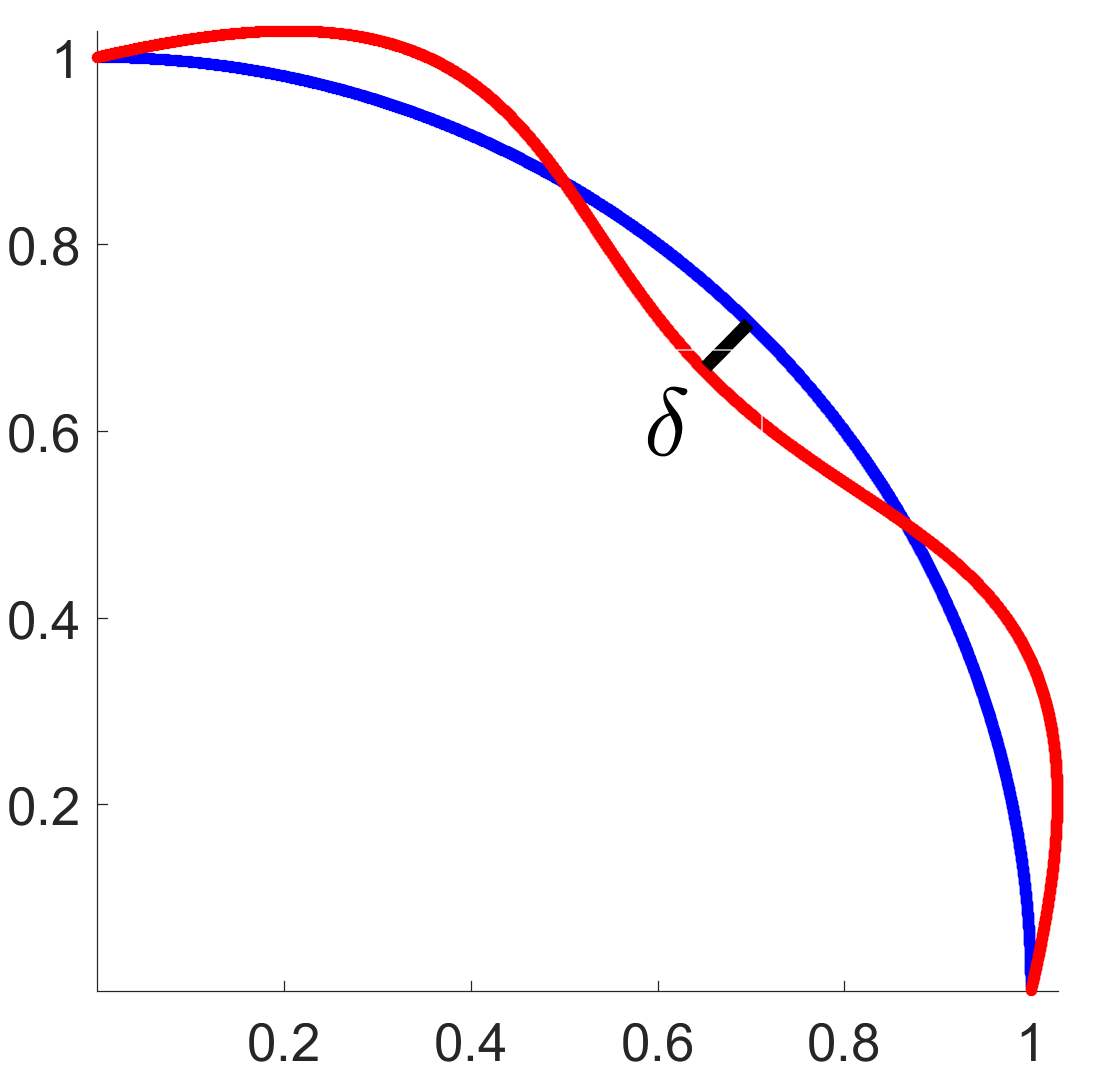
The data is like in Figure 1, where and are supported on two arcs in separated by a gap of size at various regions. We begin by specifying a reference set and the covariance field . For simplicity, we do this by uniformly sampling reference points from (see Figure 1). At each reference point , we take neighbors to estimate the local covariance matrix by . The empirical histograms and are computed as in Eqn. (2) at every point (see Figure 1), as well as the quantity as in Eqn. (4). We also compute under a permutation of the data points in and so as to mimic the null hypothesis , and we call the two values and respectively. The experiment is repeated 100 times, where , and the distribution of and are shown as red and blue bars in Figure 1. The simulation is done across three datasets where takes value as , and we compare isotropic and anisotropic kernels. When , the distributions of and overlay each other, as expected. When , greater separation between distributions of and implies greater power for the test. The advantage of the anisotropic kernel is clearly demonstrated, particularly when (the middle row).
The analysis of the testing power of hinges on the singular value decomposition of , formally written as and will be defined in Section 3. The histogram thus becomes
and similarly for , which means that the ability of to distinguish and is determined by the amount that and differ when projected onto the singular functions . For the example above, the first few singular functions are visualized in Figure 1, where the ’s of the anisotropic kernel project along the directions where and deviate at a lower index of , thus contributing more significantly to the quantity . Figure 1 also shows the “witness function” ([12], c.f. Section 2.3) of kernels, which indicates the regions of deviation between and .
Throughout the paper, we refer to the use of a local Mahalanobis distance with as an anisotropic kernel and as an isotropic kernel. Similarly, we refer to a kernel measuring affinity from all points to a reference set (i.e. ) as an asymmetric kernel. The analysis in Section 3 is for the symmetrized version of the kernel , while in practice one never computes the -by- kernel but only the -by- asymmetric kernel which is equivalent and way more efficient. We discuss more about computation in Section 4.4.
1.2 Related Work
The question of two sample testing is a central problem in statistics. In one dimension, one classical approach to two sample testing is the Kolmogorov-Smirnov distance, which compares the distance between the two empirical cumulative distribution functions [17, 25]. While there exist generalizations of these infinitely supported bins in high dimensions [4, 11, 22, 14], these require a large computational cost for either computing a minimum spanning tree or running a large number of randomized tests. This warranted binning functions that are defined more locally and in a data-adaptive fashion. Another high-dimensional extension of Kolmogorov-Smirnov is to randomly project the data into a low-dimensional space and compute the test in each dimension.
The 1D Kolmogorov-Smirnov statistic can be seen as a special case of the MMD discrepancy, which is generally defined as
where is certain family of integrable functions. When equals the set of all indicator functions of intervals in , the MMD discrepancy gives the Kolmogorov-Smirnov distance. Kernel-based MMD has been studied in [12], where the function class consists of all functions s.t. , where indicates the norm of the Hilbert space associated with the reproducing kernel. Specifically, suppose the PSD kernel is , the (squared) RKHS MMD can be written as
| (5) |
and can be estimated by (here we refer to the biased estimator in [12] which includes the diagonal terms)
The methodology and theory apply to any dimensional data as long as the kernel can be evaluated.
We consider a kernel of the form and its variants, where is certain measure of the reference points. This can be seen as a special case of RKHS MMD [12], which considers a general PSD kernel . When and is isotropic, is the Lebesgue measure, is reduced to gaussian kernel. However, returning to the asymmetric kernel as we do, allows us to easily redefine the local geometry around reference points and incorporate the local dimensionality reduction in (1). While the asymmetric kernel requires the additional technical assumption that the eigenmodes of the kernel do not vanish on the support of and , which is discussed in [12] in reference to isotropic Parzen windows, the construction yields a more powerful test for distributions that are concentrated near locally low-dimensional structures. Theoretically, our analysis gives a comparison of the testing power of different kernels, which turns out to be determined by the spectral decomposition of the kernels. This analysis augments that in [12]: the asymptotic results in [12] does not imply testing power in high dimensions, as pointed out later by [21]. Our analysis makes use of the spectral decomposition of the kernel with respect to the data distribution. While the empirical spectral expansion of translation-invariant kernels has been previously used to derive two-sample statistics, e.g. in [10] and more recently in [6, 27], and the idea dates back to earlier statistical works (see e.g. [9]), our setting is different due to the new construction of the kernel.
We generalize the construction by considering a family of kernels via a “spectral filtering”, which truncates the spectral decomposition of the anisotropic kernels and modifies the eigenvalues, c.f. Section 2.2. The modified kernel may lead to improved testing power for certain departures. The problem of optimizing over kernels has been considered by [13], where one constructs a convex combination of a finite number of kernels drawn from a given family of kernels. The family of kernels considered in [13] are isotropic kernels, and possibly linear time computed kernels with high variance, which has the effect of choosing better spectral filters for separating two distributions. However, because the kernels we consider are anisotropic, they lie outside the family of kernels considered in [13] and, in particular, have fundamentally different eigenfunctions over which we build linear combinations. Also, building spectral filters directly on the eigenfunctions yields a richer set of filters than those that can be constructed by finite convex combinations.
Our approach is also closely related to the previous study of the distribution distance based on kernel density estimation [1]. We generalize the results in [1] by considering non-translation-invariant kernels, which greatly increases the separation between the expectation of under the null hypothesis and the expectation of under an alternative hypothesis. Moreover, it is well-known that kernel density estimation, which [1] is based on, converges poorly in high dimension. In the manifold setting, the problem was remedied by normalizing the (isometric) kernel in a modified way and the estimation accuracy was shown to only depend on the intrinsic dimension [20]. Our proposed approach takes extra advantage of the locally low dimensional structure, and obtains improved distinguishing power compared to the one using isotropic kernels when possible.
At last, the proposed approach can be viewed as related to two sample testing via nearest neighbors [15]. In [15], one computes the nearest neighbors of a reference point to the data and derives a statistical test based on the amount the empirical ratio , where is the number of neighbors from (similarly ), deviates from the expected ratio under the null hypothesis, namely . Because the nearest neighbor algorithm is based on Euclidean distance, it is equivalent to a kernel-based MMD with a hard-thresholded isotropic kernel. The approach can be similarly combined with a local Mahalanobis distance as we do, which has not been explored.
2 MMD Test Statistics and Witness Functions
Given two independent datasets and , where has i.i.d. samples drawn from distribution , and has i.i.d samples drawn from , we aim to (i) test the hypothesis against the alternative, and (ii) when , detect where the two distributions differ. We assume that and are supported on compact subset of , and both distributions have continuous probability densities, so we also use and to denote the densities and write integration w.r.t. as and similarly for .
As suggested in Section 1.1, the reference set and the covariance field are important for the construction of the anisotropic kernel. In this section and next, we assume that is given and is pre-defined. In practice, will be computed by a preprocessing procedure, and can be estimated by local PCA if not given a priori, c.f. Section 4.
2.1 Kernel MMD statistics
Using the kernel defined in (1), we consider the following empirical statistic:
| (6) |
where and are defined in (2). Note that (6) assumes the measure along with the covariance field needed in (1). can be any distribution in general, and in practice, it is an empirical distribution over the finite set , i.e. , where is the number of points in . For now we leave to be general. The population statistic corresponding to (6) is
| (7) |
can be viewed as a special form of RKHS MMD: by (5), (6) is the (squared) RKHS MMD with the kernel
| (8) |
The kernel (8) is clearly positive semi-definite (PSD), however, not necessarily “universal”, meaning that the population MMD as in (7) being zero does not guarantee that . The test is thus restricted to the departures within the Hilbert space (Assumption 2).
We introduce a spectral decomposition of the kernel based upon that of the asymmetric kernel , which sheds light on the analysis: Let be a distribution of data point (which is a mixture of and to be specified later). Since is bounded by 1, so is the integral , and thus the asymetric kernel is Hilbert-Schmidt and the integral operator is compact. The singular value decomposition of with respect to and can be written as
| (9) |
where , and are ortho-normal sets w.r.t and respectively. Then (8) can be written as
| (10) |
This formula suggests that the ability of the kernel MMD to distinguish and is determined by (i) how discriminative the eigenfunctions are (viewed as “feature extractors”), and (ii) how the spectrum decay (viewed as “weights” to combine the differences extracted per mode). It also naturally leads to generalizing the definition by modify the weights , which is next.
2.2 Generalized kernel and spectral filtering
We consider the situation where the distributions and lie around certain lower-dimensional manifolds in the ambient space, and both densities are smooth with respect to the manifold and decay off-manifold, which is typically encountered in the applications of interest (c.f. Section 5). Meanwhile, since the reference set is sampled near the data, is also centered around the manifold. Thus one would expect the population histograms and to be smooth on the manifold as well. This suggests building a “low-pass-filter” for the empirical histograms before computing the distance between them, namely the MMD statistic.
We thus introduce a general form of kernel as
| (11) |
where is a sequence of sufficiently decaying positive numbers, the requirement to be detailed in Section 3. Our analysis will be based on kernels in form of (11), which includes as a special case when . While the eigenfunctions are generally not analytically available, to compute the MMD statistics one only needs to evaluate ’s on the data points in , which can be approximated by the empirical singular vectors of the -by- kernel matrix and computed efficiently for MMD tests (c.f. Section 4). Note that the approximation by empirical spectral decomposition may degrade as increases, however, for the purpose of smoothing histograms one typically assigns small values of for large so as to suppress the “high-frequency components”.
The construction (11) gives a large family of kernels and is versatile: First, setting for some positive integer is equivalent to using the kernel as where . This can be interpreted as redefining the affinity of points and by allowing -steps of “intermediate diffusion” on the reference set, and thus “on the data” [7]. When is uniform over the whole ambient space, raising is equivalent to enlarging the bandwidth of the gaussian kernel. However, when is chosen to adapt to the densities and , then the kernel becomes a data-distribution-adapted object. As increases, decays rapidly, which “filters out” high-frequency components in the histograms when computing the MMD statistic, because . Generally, setting to be a decaying sequence has the effect of spectral filtering. Second, in the case that prior knowledge about the magnitude of the projection is available, one may also choose accordingly to select the “important modes”. Furthermore, one may view the kernel MMD with (11) as a weighted squared-distance statistics after projecting to the spectral coordinates by , where the coordinates are uncorrelated thanks to the orthogonality of . We further discuss the possible generalizations in the last section. The paper is mainly concerned with the kernel , including , with anisotropic , while the above extension of MMD may be of interest even when is isotropic.
2.3 Witness functions
Following the convection of RKHS MMD [12], the “witness function” is defined as
where and are the mean embedding of and in respectively. By Riez representation, equals multiplied by a constant. We will thus consider as the witness function. By definition, , and similarly for , thus . We then have that for the statistic ,
| (12) |
and generally for ,
| (13) |
The computation of empirical witness functions will be discussed in Section 4.2.
Although the witness function is not an estimator of the difference , it gives a measurement of how and deviate at local places. This can be useful for user interpretation of the two sample test, as shown in Section 5. The witness function augments the MMD statistic, which is a global quantity.
2.4 Kernel parameters
If the reference distribution and the covariance field are given, there is no tuning parameter to compute -MMD (c.f. Algorithm 2). To compute -MMD with general , which is truncated to be of finite rank , the number and the values are tunable parameters (c.f. Algorithm 3).
If the covariance field is provided up to a global scaling constant by , e.g., when estimated from local PCA, which means that one uses for some in (1), then this is a parameter which needs to be determined in practice.
Generally speaking, one may view the reference set distribution and the covariance field as “parameters” of the MMD kernel. The optimization of these parameters surely have an impact on the power of the MMD statistics, and a full analysis goes beyond the scope of the current paper. At the same time, there are important application scenarios where pre-defined and are available, e.g., the diffusion MRI imaging data (Section 5.3). We thus proceed with the simplified setting by by assuming pre-defined and , and focusing on the effects of anisotropic kernel and re-weighted spectrum.
3 Analysis of Testing Power
We consider the population MMD statistic of the following form
| (14) |
where as in (11), and particularly as in (10). The empirical version is
| (15) |
where and , and . We consider the limit where both and go to infinity and proprotional to each other, in other words, and , and .
We will show that, under generic assumptions on the kernel and the departure , the test based on is asymptotically consistent, which means that the test power as (with controlled false-positive rate). The asymptotic consistency holds when is allowed to depend on as long as decays to 0 slower than . We also provide a lower bound of the power based based upon Chebyshev which applies to the critical regime when is proportional to . The analysis also provides a quantitative comparison of the testing power of different kernels.
3.1 Assumptions on the kernel
Because is uniformly bounded and Hilbert-Schmidt, is positive semi-definite and compact, and thus can be expanded as in (10) where are a set of ortho-normal functions under . By that , we also have that satisfies that
| (16) |
and for any . Meanwhile, is continuous (by the continuity and uniformly boundedness of ), which means that the series in (10) converges uniformly and absolutely, and the eigenfunctions are continuous (Mercer’s Theorem). Finally, (16) implies that the operator is in the trace class, and specifically .
These properties imply that when replacing by as in (11), one can preserve the continuity and boundedness of the kernel. We analyze kernels of the form as (11), and assume the following properties.
Assumption 1.
The in (11) satisfy that , , and that the kernel is PSD, continuous, and for all .
As a result, Mercer Theorem applies to guarantee that the spectral expansion (11) converges uniformly and absolutely, and the operator is in the trace class. Note that Assumption 1 holds for a large class of kernels, including all the important cases considered in this paper. The previous argument shows that is covered. Another important case is the finite-rank kernel: that is, when for some positive integer , and can be any positive numbers when such that and for all .
For the MMD test to distinguish a deviation from , it needs to have for such . We consider the family of alternatives which satisfies the following condition.
Assumption 2.
When , there exists s.t. and . In particular, if are strictly positive for all , then satisfies that does not vanish w.r.t , i.e. .
The following proposition, proved in the Appendix, shows that for such deviated .
Proposition 3.1.
Notations as above, for a fixed , the following are equivalent
(i) ,
(ii) For some , and .
If for all , then (i) is also equivalent to
(iii) .
Note that satisfies for all , thus (iii) applies. The proposition says that distinguishes an alternative when lies in the subspace spanned by , and for general , needs to lie in the subspace spanned by . These bases are usually not complete, e.g., when the reference set has points then is of rank at most . However, when the measure is continuous and smooth, the singular value decomposition (9) has a sufficiently decaying spectrum, and the low-frequency ’s can be efficiently approximated with a drastic down sampling of [3]. This means that, under certain conditions of (sufficiently overlapping with and regularity), after replacing the continuous by a discrete sampling in constructing the kernel, an alternative violates Assumption 2 only when the departure lies entirely in the high-frequency modes w.r.t the original . In the applications considered in this paper, these very high-frequency departures are rarely of interest to detect, not to mention that estimating for large lacks robustness with finite samples. Thus Assumption 2 poses a mild constraint for all practical purposes considered in this paper, even with the spectral filtering kernel which utilizes a possibly truncated sequence of .
3.2 The centered kernel
We introduce the centered kernel under , defined as
| (17) |
where , and . The spectral decomposition of is the key quantity used in later analysis.
The following lemma shows that the MMD statistic, both the population and the empirical version, remains the same if is replaced by . The proof is by definition and details are omitted.
The kernel also inherits the following properties from , proved in Appendix A:
Proposition 3.3.
The kernel , as an integral operator on the space with the measure , is PSD. Under Assumption 1,
(1) for any , and for any ,
(2) is continuous,
(3) is Hilbert-Schmidt as an operator on and is in the trace class. It has the spectral expansion
| (20) |
where , . are continuous on , are both summable and square summable, and the series in (20) converges uniformly and absolutely.
(4) The eigenfunctions are square integrable, and thus integrable, w.r.t. . Furthermore, .
3.3 Limiting distribution of and asymptotic consistency
Consider the alternative for some fixed , . remains a probability density for any . We define the constants
| (24) |
where are finite by the integrability of under ((4) of Proposition 3.3), and .
The theorem below identifies the limiting distribution of under various order of , which may decrease to 0 as . The techniques very much follow Chapter 6 of [23] (see also Theorem 12, 13 in [12]), where the key step is to replace the two independent sets of summations in (23) by normal random variables via multi-variate CLT (Lemma A.1), using a truncation argument based on the decaying of . The proof is left to Appendix A.
Theorem 3.4.
Let may depend on , , and notations , , and others like above. Under Assumption 1, as with , ,
(1) If , (including the case when ), then
Due to the summability of the random variable on the right rand side is well-defined.
(2) If , where , then
where .
(3) If , then
where , with .
Remark 3.5.
As a direct result of Theorem 3.4 (1), under ,
When , the limiting density is where are i.i.d. random variables. Theorem 3.4 (3) shows the asymptotic normality of under . One can verify that when , , where . These limiting densities under recover the classical result of V-statistics (Theorem 6.4.1.B and Theorem 6.4.3 [23]).
The numerical experiments in Section 3.5 show that the theoretical limits identified in Theorem 3.4 (1) approximate the empirical distributions of quite well when equals a few hundreds (Fig. 2). In below, we address the asymptotic consistency of the MMD test, and the finite-sample bound of the test power will be discussed in the next subsection.
A test based on the MMD statistic rejects whenever exceeds certain threshold . For a target “level” (typically ), a test (with samples) achieves level if , and the “power” against an alternative is defined as . We define the test power at level as
| (25) |
The threshold needs to be sufficiently large to guarantee that the false-positive rate is at most , and in practice it is a parameter to determine (c.f. Section 4.1). In below, we omit the dependence on in the notation, and write as . The test is called asymptotically consistent if as . For the one-parameter family of , the following theorem shows that, if satisfies Assumption 2, the MMD test has a nontrivial power when converges to a positive constant, and is asymptotically consistent if .
3.4 Non-asymptotic bound of the testing power
In this section, we derive a non-asymptotic (lower) bound of the testing power for finite , which shows that the speed of the convergence is at least as fast as as increases whenever is greater than certain threshold value.
Theorem 3.7.
Notations , , as above. Define , , and , and let be the target level. Under Assumption 1 and 2, define . If and
| (26) |
then
| (27) |
where
In particular, assuming that is uniformly bounded to be between for some , then the constants , , , are all uniformly bounded with respect to by constants which only depend on and .
The above bound applies when is proportional to , which is the critical regime. The lower bound of in (27) increases with and approaches 1 when , showing the same behavior as Theorem 3.6. It can be used as another way to prove Theorem 3.6 (2). In particular, as increases (or increases, since stays bounded) and assuming uniformly bounded , the r.h.s of (27) is dominated by
which leads to an bound of for fixed . The theorem only uses Chebyshev, so the bound may be improved, e.g., by investigating the concentration of which is a quadratic function of independent sums, c.f. (23).
We notice two other possible ways of deriving non-asymptotic bound of the power: (1) Berry-Essen rate of the convergence to asymptotic normality has been proved for U-statistics in the case of , and can be extended to the V-statistics (for the case of ), c.f. Chapter 6 of [23]. This can lead to a control of , where the constant depends on the kernel and the departure magnitude . However, when is proportional to , the Berry-Essen rate loses sharpness and cannot give a nontrivial bound. (2) Large deviation bounds of the empirical MMD have been obtained by McDiarmid inequality and the boundedness of the Rademacher complexity of the unit ball in the RKHS, where is proved to converge to the population value at the rate with exponential tail (Theorem 7 of [12]). This gives a stronger concentration than Chebyshev when for some constant and leads to an exponential decay of with increasing , but it does not apply to give a control when is proportional to i.e. the critical regime.
3.5 Comparison of kernels


As suggested by Theorem 3.7, the power of the MMD test depends on the mean and variance of the statistic under and respectively, which are
By Theorem 3.4 (1), at the critical regime where is proportional to , they can be approximated by the following (recall that )
where i.i.d. Notice that the gap , which is the population .


In this subsection, we compare isotropic and anisotropic kernels by numerically computing the above quantities under a specific choice of data distributon. We will consider three kernels: (1) the gaussian kernel (2) the one induced by the anisotropic kernel where is set to be the Lebesgue measure, and is constructed so that the tangent direction is the first principle direction with variance , and the the normal direction is the second principle direction with variance , and (3) the spectral filtered kernel as in Eqn. (11) where are designed to be 1 for and smoothly decays to zero at . All kernels are multiplied by a constant to make the largest eigenvalue so as to be comparable. We also adopt the ratio (similar to the object of kernel optimization considered in [13])
to illustrate the testing power, where the larger the the more powerful the test is likely to be.
For the distribution and , we use the 2-dimensional example in the first section of the paper. Specifically, is the uniform distribution on the curve convolved with , , and is the distribution of the shifted curve convolved with , where . One realization of 200 points in and is shown in Figure 4. 11 1 Strictly speaking and are longer compacted supported due to convolving with the 2-dimensional gaussian distribution, however, the normal density exponentially decays and is small, so that there is not any practical difference. The analysis can extend by a truncation argument. Let , we consider the one-parameter family of alternative , and will simulate in the critical regime where the test power is less than 1. We assume that and denote by in this subsection.
In all experiments, the quantities , , and are computed by Monte-Carlo simulation over 10000 runs. Their asymptotic version (with bar) are computed by 50000 draws of the limiting distribution, truncating the summation over to the first 500 terms; the values of and are approximated by the empirical eigenvalues and mean of eigenvectors over 10000 sample points drawn from and ( is computed by Nystrom extension). The values of and are shown in Figure 3, and those of etc. in Table 1.
| Gaussian | 0.4771 | 0.5444 | 0.0677 | 0.0704 | 0.4874 |
|---|---|---|---|---|---|
| 0.4754 | 0.5439 | 0.0676 | 0.0736 | 0.4848 | |
| 0.0489 | 0.0958 | 0.0214 | 0.0306 | 0.9000 | |
| 0.0488 | 0.0939 | 0.0214 | 0.0312 | 0.8573 | |
| 0.0985 | 0.2046 | 0.0348 | 0.0587 | 1.1351 | |
| 0.0983 | 0.2013 | 0.0374 | 0.0620 | 1.0354 | |
| Gaussian | 0.2381 | 0.2720 | 0.0334 | 0.0359 | 0.4885 |
| 0.2379 | 0.2722 | 0.0339 | 0.0368 | 0.4850 | |
| 0.0243 | 0.0477 | 0.0107 | 0.0153 | 0.8972 | |
| 0.0244 | 0.0471 | 0.0106 | 0.0157 | 0.8616 | |
| 0.0490 | 0.1036 | 0.0177 | 0.0305 | 1.1343 | |
| 0.0490 | 0.1003 | 0.0188 | 0.0310 | 1.0290 |
4 Practical Considerations
Algorithm 1 gives the pseudo code for two-sample test based on the proposed MMD statistics, where two external subroutines, akMMD and akWitness, will be given in Algorithm 2 and Algorithm 3 for and statistics respectively. In Algorithm 3, an extra input parameter , which is a positive vector of length (), is needed. is the target spectrum of the kernel in Eqn. (11). Both algorithms compute the threshold , which is the maximum threshold to guarantee level (controlled false discovery), by bootstrapping. It is also assumed that the reference set with are predefined.
In the rest of the section, we explain the bootstrapping approach, the empirical estimator of the witness function, and the construction of reference set in detail. We close the section by commenting on the computation complexity.
Input: Datasets and , function handle , , data points
Output: Acceptance/Rejection of , the witness function evaluated on
External: Subroutines akMMD, akWitness
4.1 Permutation test and choice of the threshold
The MMD statistics introduced in Section 3 is non-parametric, which means that the threshold does not have a closed-form expression for finite . In practice, one may use a classical method known as the permutation test [16], which is a bootstrapping strategy to empirically estimate , and previously used in RKHS MMD [12]. The idea is to model the null hypothesis by pooling the two datasets, resampling from that pool, and computing one instance of the MMD under that null hypothesis. Repetitive resampling thus corresponds to permuting the joint dataset multiple times, and it generates a sequence values of of , the -quantile of which is used as (see both Algorithm 2 and Algorithm 3). Strictly speaking, the power of the test is slightly degraded due to the empirical estimate of the null hypothesis. However, as we see in Section 5, the test still yields very strong results in a number of examples.
Meanwhile, the limiting distribution of the statistics appears to well approximate the empirical one under , as shown in Section 3.5. This suggests the possibility of determining based on the empirical spectral decomposition of the kernel. In the current work we focus on the bootstrapping approach (permutation test) for simplicity.
4.2 Empirical witness functions
The population witness functions have been introduced in Section 2.3, and, by definition, can be evaluated at any data point . For the kernel , the empirical version of Eqn. (12) is
| (28) |
which can be computed straightforwardly from the empirical histograms , and the pre-defined kernel , see Algorithm 2.
4.3 Sampling of the reference set
In bio-informatics applications e.g. flow cytometry, datasets are usually large in volume so that one can construct the reference set and covariance field from a pool of data points, which combines multiple samples, before the differential analysis in which MMD is involved. In some application scenario (like diffusion MRI), and are provided by external settings. Thus we treat the procedure of constructing and separately from the two-sample analysis, which is also assumed in the theory.
In experiments in this work, we sample the reference points randomly in Lebesgue measure using the following heuristic: given a pool of data points e.g. drawn from and or subsampled from larger datasets, the procedure loops over batches until points have been generated. In each loop, a batch of points are loaded from the pool, and candidate points are sampled from the batch according to which is the KDE of each point in the batch. The candidate points are giggled, and points which have too few neighbors in the pool dataset are excluded. The code can be found in the software github repository https://github.com/AClon42/two-sample-anisotropic.
The covariance fielded is computed by local PCA, when needed. This is related to the issue of “-selection” in gaussian MMD [12], where a “median heuristic” was proposed to determine the in the gaussian kernel . In our setting, the extension of “” is the local covariance matrix , which allows different at different points, apart from different along different local directions. In estimating , a controlling parameter is then the size of the local neighborhood, i.e. the -nearest neighbors from which local PCA is computed. In the manifold setting, there are strategies to choose so as to most efficiently estimate local covariance matrix, see e.g. [19], and it is best done by using different at different point. For simplicity, in all the experiments we set to be a fraction of the total number of samples, which may be sub-optimal. We also introduce a parameter and set , where is computed via local PCA, so as to make the “size” of tunable. The parameter is sampled on a binary grid ( for ).
4.4 Computational complexity
We will only discuss the cost of computing the MMD statistics, namely that of MMD-L2 (Algorithm 2) and MMD-Spec (Algorithm 3). The extra cost for computing the witness function is negligible, as can be seen from the code (some computation, e.g. that of and in Witness-L2, and the SVD of in Witness-spec are repetitive for illustrative purpose.)
We firstly discuss MMD-L2: The cost for computing one empirical MMD statistics is of , where is the size of the two samples. The main cost is the one-time construction of the asymmetric kernel matrix , which also dominates the memory requirements. While the choice of the reference set, and hence the number of reference points , is related to the problem being addressed, any amount of structure in the samples leads to a choice of that is . This yields major computational and memory benefits as the test complexity is much smaller than the , which is the order for computing the U-statistics via a symmetric gaussian kernel without extra techniques. In all applications we’ve considered and synthetic examples we’ve worked with, is in the tens or hundreds, and can remain relatively constant as grows while still yielding a test with large power. This means the test with an anisotropic kernel becomes linear in the number of points being tested.
In MMD-spec, the extra computation is for the rank- SVD of the -by- matrix . The computation can be done in time via the classical pivoted QR decomposition, and may be accelerated by modern randomized algorithms, e.g. the approach in [26] which takes time to achieve an accuracy proportional to the magnitude of the )-th singular value. The computational cost may be furtherly reduced by making use of the sparse/low-rank structure of the kernel matrix when possible. When the kernel almost vanishes outside a local neighborhood of which has at most points, the rows of are -sparse, and then fast nearest neighbor search methods (by Kd-tree or randomized algorithm) can be applied under the local Mahalanobis distance and the storage is reduced to . When has a small numerical rank, e.g. only singular values are significantly nonzero, can be stored in its rank- factorized form which can be computed in linear time of . This will save computation in bootstrapping as both and can be computed from and (row-permuted) only.
5 Applications
5.1 Synthetic examples
5.1.1 Example 1: Curve in 2 dimension
 |
 |
 |
 |
 |
| A1 | A2 | A3 | A4 | A5 |
The density is the uniform distribution on a quarter circle with radius 1 convolved with , on a quarter circle with radius convolved with , which is the same example in Section 3.5 (top left in Figure 2), . The departure is parametrized by , taking values from 0 to 0.02. The rejection rate is computed from the average over runs according to Algorithm 1, as shown in the left of Figure 4, where the errorbars indicate the standard deviation. For the gaussian kernel, the curve corresponds to the which has the best performance over a grid, and it is obtained by an intermediate value on the grid. The witness functions of the three kernels when are computed according to Section 4.2, and shown in Figure 4.
5.1.2 Example 2: Gaussian mixture in 3 dimension
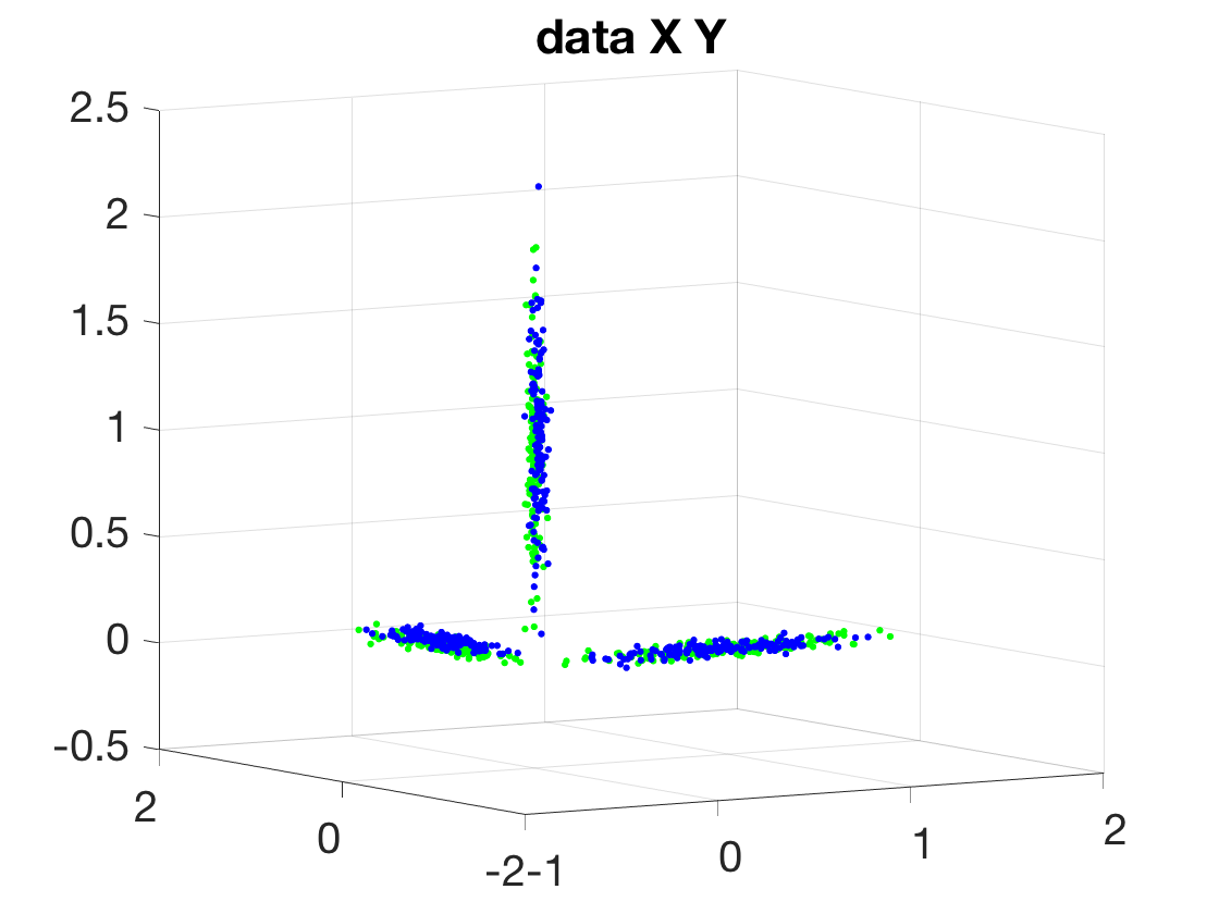


Two gaussian mixtures in , , . The density consists of 3 equal-size components centering at , and respectively, with diagonal covariance matrix , and , ; and density differs from by centering the three means at , and , while letting the covariance matrices remain the same. The constant takes value from 0 to 0.02. Results shown in Figure 5, similar to Figure 4.
5.2 Flow cytometry data analysis
Flow Cytometry is a laser based technology used for cell counting. It is routinely used in diagnosing blood diseases by measuring various physical and chemical characteristics of the cells in a sample. This leads to each sample being represented by a multi-dimensional point cloud of tens of thousands of cells that were measured.
Two natural questions arise in comparing various flow cytometry samples. The first is a supervised learning question: can a statistical test detect the systemic differences between a set of healthy people and a set of unhealthy people? The second question is an unsupervised learning question: can the distance measure be used to determine the pairwise distance between any two samples, and will that distance matrix yield meaningful clusters?
We address both of these questions for two different flow cytometry datasets. We compare isotropic gaussian MMD to anisotropic MMD and demonstrate, in all cases, our anisotropic MMD test has more power and yields more accurate unsupervised clusters. We only show the pairwise distance embedding for the reference set asymmetric kernel due to the untenable cost of computing each of the pairs.
5.2.1 AML dataset
 |
 |
 |
| A1 | A2 | B1 |
 | ||
| A3 | A4 | B2 |
Acute myeloid leukemia (AML) is a cancer of the blood that is characterized by a rapid growth of abnormal white blood cells. While being a relatively rare disease, it is incredibly deadly with a five-year survival rate of [8]. AML is diagnosed through a flow cytometry analysis of the bone marrow cells, and while there are features that distinguish AML in certain cases, other cases can be more difficult to detect. State of art supervised methods include SPADE, Citrus, etc. See [5] and the references therein.
The data is from the public competition Flow Cytometry: Critical Assessment of Population Identification Methods II (FlowCAP-II). This dataset consists of 316 healthy patients and 43 patients with Acute myeloid leukemia (AML), where each person has approximately cells measured across 7 physical and chemical features.
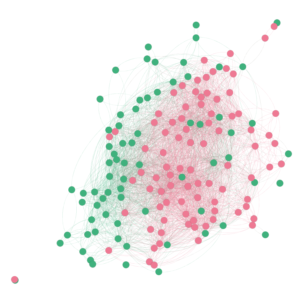
We use an anisotropic kernel with only reference points. We create an unsupervised clustering by computing the pairwise distances between person and person . In Figure 6, we display the network of these people constructed by weighting each edge as the exponential of the negative distance properly scaled. When supervising the process and running a two sample test between the pool of healthy cells and the pool of unhealthy cells, we see that the anisotropic kernel yields significantly better separation and lower variance than the isotropic gaussian kernel.
We also examine the witness function in Figure 6 that is generated by the anisotropic kernel, as introduced in Section 2.3. This yields a tool for visualizing the separation between the two samples in the original data space. This gives a way to communicate the decision boundary to the medical community, which uses visualization of the 2D slices as the diagnostic tool for determining whether the patient as AML.
5.2.2 MDS dataset
Myelodysplastic syndromes (MDS) are a group of cancers of the blood. There is more variability in how MDS presents itself in the cells and flow cytometry measurements. The data we work with came from anonymized patients that were treated at Yale New Haven Hospital. After choosing to examine surface markers CD16, CD13, and CD11B, along with several physical characteristics of the cells, we’re left with 72 patients that were initially diagnosed with some form of MDS and 87 patients that were not. These patients are represented by about cells in 8 dimensions.
While MDS is more difficult to detect than AML, the unsupervised pairwise graph, created the same way as in Figure 6, still yield a fairly strong unsupervised clustering, as we see in Figure 7. When supervising the process and running a two sample test between the pool of healthy cells and the pool of unhealthy cells, we see that the anisotropic kernel yields strongly significant separation between the two classes, unlike the isotropic gaussian kernel.
 |
 |
 |
 |
| A1 | A2 | A3 | A4 |
5.3 Diffusion MRI imaging analysis
 |
 |
 |
 |
 |
| A1 | A2 | B1 | B2 | B3 |
 |
 |
 |
 |
 |
| A3 | A4 | B4 | B5 | B6 |
 |
 |
 |
 |
 |
| A5 | A6 | B7 | B8 | B9 |
Diffusion weighted MRI is an imaging modality that creates contrast images via the diffusion of water molecules. Various regions of the brain diffuse in different ways, and the patters can reveal details about the tissue architecture. At a low level, each pixel in a 3D brain image generates a 3D diffusion tensor (i.e. covariance matrix) that describes the local flow of water molecules.
An important question in diffusion MRI analysis is to identify regions of the brain that systemically differ between groups of healthy and sick individuals. We attack this problem by comparing the distributions of the diffusion tensors in various regions of the brain, thus framing it as a multiple sample problem. Every brain is co-registered so that the pixels overlap.
Real images are around , so the amount of memory needed to build a square symmetric kernel, even a sparse one, is completely prohibitive. For this reason, we instead consider a set of reference pixels that subsamples the image, and construct a anisotropic kernel , where is the location of pixel and is the diffusion tensor at pixel . This kernel must enforce both locality in the pixel space, and the local behavior of the diffusion tensors. The latter requires measuring covariance matrices over the space of positive semi-definite matrices.
Fortunately, the study of covariance matrices on the space of positive semi-definite matrices is a well studied phenomenon [2]. The main takeaway is that there is an isomorphism from a diffusion tensor and its vectorized representation
Thus, we can define a covariance matrix on and define the anisotropic kernel
| (30) |
We examine MMD using a synthetic data set generated from the common brain phantom image. We treat this as a 2D slice of the 3D image, and simply have all tensor variation in the z-direction constant and uncorrelated with the xy-direction of this slice. We also assume that the brains have been co-registered. The process of co-registration is an independent preprocessing issue which can be incorporated into our proposed methodology when working with real world data sets, but is outside the scope of this paper.
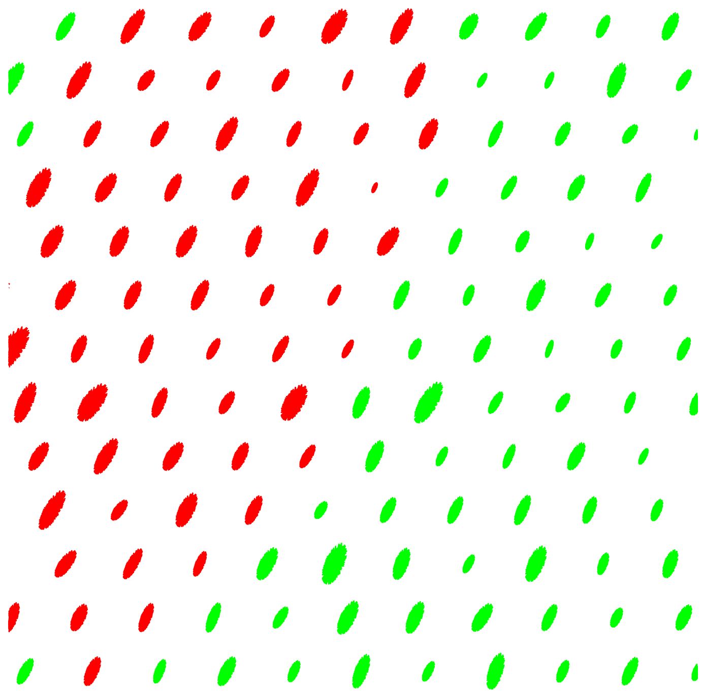
In Figure 8, we show both a “healthy” brain and an “unhealthy” brain in which a small region has been removed. The intensity of the image in this case will correspond to the eccentricity of the diffusion tensor at that point; the magnitude of the tensor will decrease from left to right in the same way for both images and the angle shift uniformly from left to right. The eccentricity, magnitude, and angle all have iid Gaussian noise added to them with .
We down-sample the brain by a factor of 5 for the reference points, and consider the mean embeddings for realizations of a healthy brain (null hypothesis ), and for realizations of a healthy brain and realizations of an unhealthy brain (alternative hypothesis ). Figure 8 shows the supervised witness function of regions of difference between the two groups, as well as a permutation test in which we permute group labels while maintaining the individual brain structure. We also show the leading eigenvectors of the pairwise network generated by measuring the MMD between any two brains.
By using reference points, each brain is represented by a kernel that is , and the data adaptive MMD computation can be run on 10 brains in about minutes on a standard laptop.
We also compare the anisotropic kernel to one with an isotropic kernel of constant bandwidth. We cannot compare to kernel MMD with a square symmetric kernel due to computational limits, so instead we compare to the modified asymmetric kernel as in (30), but without the covariance matrix. Instead, we replace by a constant bandwidth, which is chosen to be .
6 Discussion and Remarks
The paper studies kernel-based MMD statistics with kernels of the form , and more generally, where is a “filtering” kernel over . The statistics can be computed with a pre-defined reference set in time , where is the number of samples and is the cardinal number of the reference set. The power of the test against alternative distributions is analyzed using the spectral decomposition of the kernel with respect to the data distribution, and the consistency is proved under generic assumptions. The difference in the testing power of the kernels are determined by their spectral properties. We apply the proposed methodology to flow cytometry and diffusion MRI data analysis, where the goal of analysis is formulated as comparing the distribution of multiple samples.
We close the section by a few remarks about the proposed approach as well as possible extensions:
The spectral coordinates. The kernel-MMD distance being studied can be viewed as certain distance, weighted or unweighted, in the space of spectral embedding. This is reflected in the construction of the kernel , as well as in the power analysis. Theoretically, the space of spectral embedding is infinitely dimensional, however, in practice only finite dimensional coordinates may contribute to the RKHS MMD statistic - in the sense of providing statistically significant departures. Thus, the leading coordinates of spectral embedding (depends on the kernel) gives a mapping from to , where may be proportional or larger than , and one may consider the two-sample test in the new coordinates. The general alternative then becomes a mean-shift alternative in the new coordinates. This suggests other possible tests for mean-shift alternatives than the weighted distance test being studied.
Weighting of bins. While spectral filtering introduces weighting in the generalized Fourier domain, another important variation is to introduce weighting in the “real domain”, namely weighting each bin centered at by a weight . Such weights may be computed from data, e.g. by certain local -value (see below), where the dependence among ’s needs to be handled. Another interesting question is how to introduce multi-resolution systems in the context of the current paper: Mapping points into spectral coordinates has certain advantage as analyzed in the paper, however, spectral basis is global and may not be sensitive enough to local departure. On the other hand, histograms on local bins may have large variance and one needs to jointly analyze multiple bins. The shortcomings of both approaches may be overcome by considering a multi-scale basis on the reference-set graph.
Beyond distance. RKHS MMD considers the distance by construction, while other metrics have been studied in literature, particularly the Wasserstein metric which has the interpretation of optimal flow given the underlying geometry. Such “geometric” distances are certainly useful in various application scenarios. Using the reference set, a modification of will be
| s.t. |
where , are the population histograms, and is certain metric on reference set. It may also be possible to construct a metric which is equivalent to the Wasserstein metric by measuring the difference at reference points across multiple scales of covariance matrices, as is done with with Haar wavelet [24] and with diffusion kernels [18]. Efficient estimation scheme of the Wasserstein metric needs to be developed as well as the consistency analysis with samples.
Local -value. The current approach gives a global test and computes the -value for the hypothesis of the distribution globally. In certain applications, especially differential analysis of flow cytometry data and other single-cell data, a more-important problem is to find the local region where the two samples differ corresponding to different biological conditions, or in other words, to derive a “local” -value of the test. While the witness function introduced in our current approach can provide indication where , a more systematically study of testing the hypothesis locally and controlling false discovery rate across bins is needed.
Acknowledgment
We would like to thank Yuval Kluger for introducing the problem of flow cytrometry data analysis, and Wade Schultz, Richard Torres, and Jon Astle for facilitating access to the Yale New Haven Hospital data. We would also like to thank Carlo Pierpaoli, Neda Sadeghi, and Okan Irfanoglu for introducing the problem of diffusion MRI data analysis. Cloninger was supported by NSF grant DMS-1402254.
References
- [1] Niall H Anderson, Peter Hall, and D Michael Titterington. Two-sample test statistics for measuring discrepancies between two multivariate probability density functions using kernel-based density estimates. Journal of Multivariate Analysis, 50(1):41–54, 1994.
- [2] Peter J Basser and Sinisa Pajevic. Spectral decomposition of a 4th-order covariance tensor: Applications to diffusion tensor mri. Signal Processing, 87(2):220–236, 2007.
- [3] Amit Bermanis, Amir Averbuch, and Ronald R Coifman. Multiscale data sampling and function extension. Applied and Computational Harmonic Analysis, 34(1):15–29, 2013.
- [4] Peter J Bickel. A distribution free version of the smirnov two sample test in the p-variate case. The Annals of Mathematical Statistics, 40(1):1–23, 1969.
- [5] Robert V Bruggner, Bernd Bodenmiller, David L Dill, Robert J Tibshirani, and Garry P Nolan. Automated identification of stratifying signatures in cellular subpopulations. Proceedings of the National Academy of Sciences, 111(26):E2770–E2777, 2014.
- [6] Kacper P Chwialkowski, Aaditya Ramdas, Dino Sejdinovic, and Arthur Gretton. Fast two-sample testing with analytic representations of probability measures. In Advances in Neural Information Processing Systems, pages 1981–1989, 2015.
- [7] Ronald R Coifman, Stephane Lafon, Ann B Lee, Mauro Maggioni, Boaz Nadler, Frederick Warner, and Steven W Zucker. Geometric diffusions as a tool for harmonic analysis and structure definition of data: Multiscale methods. Proceedings of the National Academy of Sciences, 102(21):7432–7437, 2005.
- [8] Barbara Deschler and Michael Lübbert. Acute myeloid leukemia: epidemiology and etiology. Cancer, 107(9):2099–2107, 2006.
- [9] TW Epps and Kenneth J Singleton. An omnibus test for the two-sample problem using the empirical characteristic function. Journal of Statistical Computation and Simulation, 26(3-4):177–203, 1986.
- [10] V Alba Fernández, MD Jiménez Gamero, and J Muñoz García. A test for the two-sample problem based on empirical characteristic functions. Computational statistics & data analysis, 52(7):3730–3748, 2008.
- [11] Jerome H Friedman and Lawrence C Rafsky. Multivariate generalizations of the wald-wolfowitz and smirnov two-sample tests. The Annals of Statistics, pages 697–717, 1979.
- [12] Arthur Gretton, Karsten M Borgwardt, Malte J Rasch, Bernhard Schölkopf, and Alexander Smola. A kernel two-sample test. Journal of Machine Learning Research, 13(Mar):723–773, 2012.
- [13] Arthur Gretton, Dino Sejdinovic, Heiko Strathmann, Sivaraman Balakrishnan, Massimiliano Pontil, Kenji Fukumizu, and Bharath K Sriperumbudur. Optimal kernel choice for large-scale two-sample tests. In Advances in neural information processing systems, pages 1205–1213, 2012.
- [14] Peter Hall and Nader Tajvidi. Permutation tests for equality of distributions in high-dimensional settings. Biometrika, 89(2):359–374, 2002.
- [15] Norbert Henze. A multivariate two-sample test based on the number of nearest neighbor type coincidences. The Annals of Statistics, pages 772–783, 1988.
- [16] James J Higgins. Introduction to modern nonparametric statistics. 2003.
- [17] A Kolmogorov. Sulla determinazione empirica di una legge di distribuzione. G. Ist. Ital. Attuari, 4:83––91, 1933.
- [18] William Leeb and Ronald Coifman. Hölder–lipschitz norms and their duals on spaces with semigroups, with applications to earth mover’s distance. Journal of Fourier Analysis and Applications, 22(4):910–953, Aug 2016.
- [19] Anna V Little, Mauro Maggioni, and Lorenzo Rosasco. Multiscale geometric methods for data sets i: Multiscale svd, noise and curvature. Applied and Computational Harmonic Analysis, 2016.
- [20] Arkadas Ozakin and Alexander G Gray. Submanifold density estimation. In Advances in Neural Information Processing Systems, pages 1375–1382, 2009.
- [21] Aaditya Ramdas, Sashank Jakkam Reddi, Barnabás Póczos, Aarti Singh, and Larry Wasserman. On the decreasing power of kernel and distance based nonparametric hypothesis tests in high dimensions. In Twenty-Ninth AAAI Conference on Artificial Intelligence, 2015.
- [22] Paul R Rosenbaum. An exact distribution-free test comparing two multivariate distributions based on adjacency. Journal of the Royal Statistical Society: Series B (Statistical Methodology), 67(4):515–530, 2005.
- [23] Robert J Serfling. Approximation theorems of mathematical statistics, 1981.
- [24] Sameer Shirdhonkar and David W Jacobs. Approximate earth mover’s distance in linear time. In Computer Vision and Pattern Recognition, 2008. CVPR 2008. IEEE Conference on, pages 1–8. IEEE, 2008.
- [25] Nickolay Smirnov. Table for estimating the goodness of fit of empirical distributions. The annals of mathematical statistics, 19(2):279–281, 1948.
- [26] Franco Woolfe, Edo Liberty, Vladimir Rokhlin, and Mark Tygert. A fast randomized algorithm for the approximation of matrices. Applied and Computational Harmonic Analysis, 25(3):335–366, 2008.
- [27] Ji Zhao and Deyu Meng. Fastmmd: Ensemble of circular discrepancy for efficient two-sample test. Neural computation, 2015.
Appendix A Proofs in Section 3
A.1 Proofs of Propositions 3.1, 3.3
Proof of Proposition 3.1.
Recall that has the singular value decomposition (9), and thus
with all strictly positive. This means that (iii) is equivalent to for some . When is all strictly positive, it is equivalent to (ii). ∎
Proof of Proposition 3.3.
We first verify the positive semi-definiteness of : for any so that , by definition,
where . The quantity is nonnegative by that is PSD.
To prove (1): Under Assumption 1, and for any . This implies the boundedness of and in (17) and leads to (1).
(2) follows from the continuity of .
The square integrability of then follows from boundedness of , which makes the operator Hilbert-Schmidt with
| (1) |
by (1). Meanwhile, by (1) again,
which proves that the operator is in trace class. Mercer’s Theorem applies to give the spectral expansion and the relevant properties, and is by the centering so that for all . This proves (3).
Finally, by the uniform convergence of Eqn. (20), and (1), , which proves (4). ∎
A.2 Proof of Theorems 3.4, 3.6
Lemma A.1 (Replacement lemma).
Let be a sequence of positive number so that . Let be an array of random variables, , , s.t. for each ,
where . Furthermore, as ,
(i) elementwise, and for any finite , where .
(ii) There exists s.t.
and the convergence is uniform in .
Meanwhile, let , , be three double arrays satisfying that
(iii) , ; as ,
(iv) There exist s.t.
for all , and the convergence is uniform in .
Then, as , the random variable
| (2) |
converges in distribution to defined as
| (3) |
and has finite mean and variance.
Proof.
Firstly, we verify that is well-defined and has finite variance: notice that (ii) implies that , (iii) implies that , , and (iv) implies that and . For finite , we define the truncated as taking the summation from to in Eqn. (3). Then
and thus
| (4) |
due to the summability of , and (the 2nd term is bounded by Cauchy-Schwarz). Thus with probability one, and . Furtherly,
by that is finite. This verifies that has finite mean and variance. Actually, by martingale convergence theorem one can show that a.s.
Secondly, using a similar argument, defining to be the truncated in Eqn. (2), one can show that
| (5) |
by that , and all converges to zero uniformly in , which is assumed in condition (ii) and (iv).
Now we come to prove . By Levy’s Continuity Theorem, it suffice to show the pointwise convergence of the characteristic function, namely
Using the truncation of up to , we have that
| (6) |
By Eqn. (4) and (5), for any , and any , we can choose sufficiently large s.t. the first and the third term are both less than for any . To show that the second term can be made small, we introduce
and by that (condition (i)), . Meanwhile,
Since is finite, and is uniformly bounded as increases for each , we have that as , by the convergence of , and . Thus the second term can be bounded by
| (7) | |||||
where (I) can be made smaller than for large ( is fixed and ), and (II) can be made smaller than as a result of which implies convergence of characteristic function. Putting together, the l.h.s. of Eqn. (6) can be made smaller than for large , which proves the claim. ∎
Proof of Theorem 3.4.
We introduce
where, by definition,
and
Using the above notations, we rewrite Eqn. (23) as
| (8) |
where and . The random variables are independent from , and both are asymptotically normal for finite many ’s. We will use the replacement lemma A.1 to substitute and by their normal counterparts, and discuss scenarios (1)-(3) respectively.
To apply Lemma A.1, we set , and the summability follows (3) of Proposition 3.3; we set
| (9) |
and then (8) becomes
| (10) |
We have that
| (11) | |||||
| (12) |
where, recalling that , , and ,
| (13) | |||||
By that and , both and are uniformly bounded, so are bounded for each . We now verify condition (i) and (ii) in Lemma A.1:
Condition (i): In case (1) and (2), , thus and then . In case (3) , thus and then . As for the limiting distribution of for any finite , we know that , and by Lindeberg-Levy CLT (Theorem 1.9.1 B in [23], extended to the case where the covariance matrix converges to a non-degenerate limit by Slutsky Theorem). By definition of and that and are independent, where () is replaced by () by Slutsky Theorem. The argument applies to all the three cases.
Condition (ii): for some absolute positive constant and . Meanwhile, by Eqn. (13), , thus
thanks to that and that ((4) of Proposition 3.3), and the convergence is uniform in .
We now consider the three scenarios respectively:
(1) Let , by Eqn. (10) we have
thus (iii) holds. Condition (iv) can be verified by that (upper bounded by ). As analyzed above, , and condition (i) and (ii) hold, thus Lemma A.1 applies to give that
as claimed in the theorem.
(2) Let be the l.h.s. of the statement, then
and condition (iii) and (iv) hold. Same as in (1), and (i) and (ii) hold, thus Lemma A.1 gives that
By the summability of , is in same distribution as as defined in the theorem.
(3) Similar to (2), let be the l.h.s. of the statement, then , , are same as in (2) where , so they have the same limit, and (iii) and (iv) hold. As analyzed above, , and (i) and (ii) hold. Thus Lemma A.1 gives that where has covariance . By the summability of , is in same distribution as , where which equals the formula claimed in the theorem. ∎
Proof of Theorem 3.6.
We only prove (2), as (1) directly follows from Theorem 3.4 (1) and the form of the limiting density of in this case.
We first consider the case, i.e. : Due to that satisfies Assumption 2 and the equivalent forms of as in (18), (22), we have that
Notations as in the proof of Theorem 3.4, by (10),
We set to be the l.h.s., and apply Lemma A.1: and are summable as before. Conditions (i) (ii) are satisfied by (defined in (9)), as has been verified in the proof of Theorem 3.4. Since
and , Condition (iii) holds with the limits as
Condition (iv) is also satisfied due the summability of , same as in the proof of Theorem 3.4. Thus Lemma A.1 gives that
| (14) |
which is a single-point distribution at the positive constant .
We then consider the case, i.e. : By Theorem 3.4 (1), which is a continuous nonnegative random variable with finite mean and variance. Thus for any chosen level , there exists s.t. , and then when is large enough,
This means that is a valid threshold in (25), and as a result, (shortening “” as )
Putting together with (14), we then have that for sufficiently large ,
which converges to 0 since is an absolute constant and thus , and meanwhile . This proves that . ∎
A.3 Proof of Theorem 3.7
Proof of Theorem 3.7.
We use Chebyshev to control the deviation of the random variable from its mean, under and respectively.
Under , , by (10),
By (12), ,
| (15) |
We will prove later that
| (16) |
and then by Chebyshev we have that for any ,
Setting the r.h.s to be gives , and thus
| (17) |
Under , by (10) and the definition that ,
| (18) | ||||
| (19) |
Since (c.f. (11)),
we have that
| (20) |
We will prove later that
| (21) |
and then, using Chebyshev again, for any ,
Combined with (17) which shows that is a valid threshold to achieve level , by setting (which is strictly positive under (26)), this gives the bound (27).
Proof of (16): We will prove that
| (22) |
where the first term since (c.f. (1)), and the second term under the condition that . This gives (16).
Recall that , and . By the definition of (9),
| (23) |
Note that
and then
| 3rd term in (23) | ||||
| (24) |
Recall that for any , thus does not vanish only when the indices all equal or fall into two pairs. Then
| (24) | ||||
| (25) |
Recall that
| (26) | ||||
| (27) |
and (c.f. Proposition 3.3 (1)), the above line continues to give that
| (28) |
Similarly, the 4th term can be bounded by
| (29) |
Back to (23), we have that
which is (22).
Proof of (30): Recall that (c.f. (12)), and ,
We define
| (33) |
and then
thus
| (34) |
Meanwhile, by Proposition 3.3 (1), uniformly, this gives that for any . Thus,
As a result,
which proves (30).
Proof of (31): By (9), the independence of from , and that , for all ,
We then have that
where is defined as
| (35) | ||||
| (36) | ||||
| (37) |
We compute and respectively: Note that , thus
due to that vanishes unless the three indices coincide. By that and , we have that
| (38) |
As for , by that for any , a similar argument gives that
To proceed, by Cauchy-Schwarz,
where, same as in (34),
and, by the uniform bound that , we also have that
| (39) |
Together, they give that
This means that
| (40) |
Back to (A.3), we have that
namely (31).