density of stable ergodicityThanks: A.A. was partially supported by the ERC Starting Grant Quasiperiodic and S.C. by the ERC Advanced Grant NUHGD. A.A. and S.C. were partially supported by the Balzan Research Project of J.Palis. A.W. was supported by NSF grant DMS-1316534.
Abstract.
We prove a version of a conjecture by Pugh and Shub: among partially hyperbolic volume-preserving diffeomorphisms, , the stably ergodic ones are -dense.
To establish these results, we develop new perturbation tools for the topology: linearization of horseshoes while preserving entropy, and creation of “superblenders” from hyperbolic sets with large entropy.
1. Introduction
A volume-preserving, diffeomorphism of a compact Riemannian manifold is stably ergodic if any volume preserving, diffeomorphism that is sufficiently close to in the topology is ergodic with respect to volume.
Interest in stably ergodic dynamical systems dates back at least to 1954 when Kolmogorov in his ICM address posited the existence of stably ergodic flows [Ko]. The first natural class of stably ergodic diffeomorphisms was established by Anosov in the 1960’s. These so-called Anosov diffeomorphisms remained the only known examples of stably ergodic diffeomorphisms for nearly 30 more years.
Grayson, Pugh and Shub [GPS] established the existence of non-Anosov stably ergodic diffeomorphisms in 1995. They considered the time-one map of the geodesic flow for a surface of constant negative curvature. These examples belong to a class of dynamical systems known as the partially hyperbolic diffeomorphisms.
A diffeomorphism is partially hyperbolic if there is a continuous splitting of the tangent bundle , invariant under the derivative , such that vectors in are uniformly expanded in length by , vectors in are uniformly contracted, and the expansion and contraction of the length of vectors in is dominated by the expansion and contraction in and , respectively. See Section 2.2 below for a precise definition.
Based on [GPS] and related work, Pugh and Shub formulated in 1996 a bold conjecture about partial hyperbolicity and stable ergodicity [PS]:
Stable Ergodicity Conjecture. Stable ergodicity is -dense among the partially hyperbolic, volume-preserving diffeomorphisms on a compact connected manifold, for any .
Restricting to the class of partially hyperbolic diffeomorphisms for which the center bundle is one-dimensional, this conjecture was proved by F. Rodriguez-Hertz, M.A. Rodriguez-Hertz and Ures [RRU]. Here we will establish, in general, a version of the Stable Ergodicity Conjecture:
Theorem A. Stable ergodicity is -dense in the space of partially hyperbolic volume-preserving diffeomorphisms on a compact connected manifold, for any .
2. Some background and structure of the proof
We fix notation to be used throughout the paper. Let be a compact, connected boundaryless manifold with a fixed Riemannian metric, and denote by the volume in this metric, normalized so that . Sometimes we will also consider a symplectic structure and its associated normalized volume . The spaces of , volume preserving and symplectic diffeomorphisms are denoted by and , respectively.
2.1. The Hopf argument and stable ergodicity
One of the earliest arguments for proving ergodicity, still in use today, was originally employed by Eberhard Hopf in the 1930’s to prove ergodicity of the geodesic flow for closed, negatively curved surfaces. These flows (“Anosov flows” in current terminogy) have one-dimensional invariant expanded and contracted distributions and , tangent to invariant foliations and , respectively. Hopf’s ergodicity argument uses the Ergodic Theorem to show that any invariant set for the flow must consist of essentially whole leaves of both and . Invariance under the flow implies that the same is true for the foliations and formed by flowing the leaves of and , respectively. Since the leaves of these foliations are transverse, a version of Fubini’s theorem implies that every invariant set for the flow must have full measure in neighborhoods of fixed, uniform size in the manifold. Ergodicity follows from connectedness and this local ergodicity. The version of Fubini’s theorem employed by Hopf is fairly straightforward, since in his setting, the foliations and (and indeed, and ) are .
Hopf himself foresaw the general usefulness of his methods beyond the geometric context of geodesic flows. In 1940 he wrote: “The range of applicability of the method of asymptotic geodesics extends far beyond surfaces of negative curvature. In [H1], -dimensional manifolds of negative curvature were already investigated. But the method allows itself to be applied to much more general variational problems with an independent variable, aided by the Finsler geometry of the problems. This points to a wide field of problems in differential equations in which it will now be possible to determine the complete course of the solutions in the sense of the inexactly measuring observer.”[H2]
Kolmogorov, too, saw the potential of the Hopf argument as a general method to prove ergodicity. In his 1954 ICM address [Ko], he wrote: “it is extremely likely that, for arbitrary , there are examples of canonical systems with degrees of freedom and with stable transitiveness [i.e. ergodicity] and mixing... I have in mind motion along geodesics on compact manifolds of constant negative curvature... ” Kolmogorov’s intuition was clearly guided by the robust nature of Hopf’s ergodicity proof; indeed, inspected carefully with a modern eye, Hopf’s original approach gives a complete proof of Kolmogorov’s assertion that the geodesic flow for a hyperbolic manifold remains ergodic when perturbed within the class of Hamiltonian (or even volume-preserving) flows.11 1 For flows that are perturbations of constant negative curvature geodesic flows, the foliations and are , which is enough to carry out the Fubini step. The same regularity of the foliations does not for geodesic flows on arbitrary negatively curved manifolds.
Around ten years later, Anosov [An1] generalized Hopf’s theorem to closed manifolds of strictly negative (but far from constant) sectional curvatures, in any dimension. The key advance was to extend the Fubini part of Hopf’s argument when the foliations and are not but still satisfy an absolute continuity property. This also gave the ergodicity of , volume-preserving uniformly hyperbolic diffeomorphisms, now known as the Anosov diffeomorphisms. These are the diffeomorphisms for which there exists a -invariant splitting and an integer such that for every unit vector :
| (1) |
Since Anosov diffeomorphisms form a -open class, and , volume-preserving Anosov diffeomorphisms are ergodic, it follows that Anosov diffeomorphisms are stably ergodic. The general expectations of Hopf and Kolmogorov were thus met in Anosov’s work. But there is more to the story: while Anosov diffeomorphisms gave the first examples of stably ergodic systems, their existence raised the question of what other examples there might be.
2.2. Dominated splittings and partial hyperbolicity: the Pugh-Shub Conjectures
Since stable ergodicity is by definition a robust property, it is natural to search for an alternate robust, geometric/topological dynamical characterization of the stably ergodic diffeomorphisms. Bonatti-Diaz-Pujals [BDP] proved a key result which can be slightly modified to show that stable ergodicity of implies the existence of a dominated splitting, that is, a -invariant splitting , and an integer such that for every unit vectors :
The stably ergodic diffeomorphisms built by Grayson, Pugh and Shub have a dominated splitting of a special type, incorporating features of Anosov diffeomorphisms: they are partially hyperbolic, meaning there exists a dominated splitting , with both and nontrivial, and an integer such that (1) holds for any unit vector . The bundles , and are called the unstable, center and stable bundles, respectively. Anosov diffeomorphisms are the partially hyperbolic diffeomorphisms for which is trivial.
As with Anosov diffeomorphisms and flows, the unstable bundle and the stable bundle of a partially hyperbolic diffeomorphism are uniquely integrable, tangent to the unstable and stable foliations, and , respectively. However, they do not span , and thus are not transverse (except in the Anosov case). The Hopf argument for local ergodicity may fail without further assumptions: there do exist non-ergodic partially hyperbolic diffeomorphisms.
As a substitute for transversality [GPS] introduced an additional assumption, a property called ‘‘accessibility,’’ which is a term borrowed from the control theory literature.22 2 Brin and Pesin had earlier studied the accessibility property and its stability properties in the 1970’s and used it to prove topological properties of conservative partially hyperbolic systems. A partially hyperbolic diffeomorphism is accessible if any two points in the manifold can be connected by a continuous path that is piecewise contained in leaves of and . Then we say that is stably accessible if any volume preserving perturbation of is accessible.
The route suggested by Pugh-Shub to prove the Stable Ergodicity Conjecture was to establish two other conjectural statements about the space of volume-preserving partially hyperbolic diffeomorphisms: 1) stable accessibility is dense, and 2) accessibility implies ergodicity.
The -density of stable accessibility remains open, except in the case of one-dimensional center bundle [RRU]. However, in the case we are concerned with, it was established by Dolgopyat and Wilkinson [DW] in 2003.
The connection between accessibility and ergodicity is certainly reasonable at the heuristic level: The Hopf argument can be carried out in the partially hyperbolic setting, and the ergodic (and even mixing) properties of the system can be reduced to the ergodic properties of the measurable equivalence relation generated by the pair of foliations . However, in trying to show that these ergodic properties follow from the assumption of accessibility, one quickly encounters substantial issues involving sets of measure zero and delicate measure-theoretic and geometric properties of the foliations.
Currently these issues can be resolved under an additional assumption called center bunching (which constrains the nonconformality of the dynamics along the center bundle ), a result due to Burns and Wilkinson [BW]. In all likelihood, a significant new idea is needed to make further progress. While including a broad range of examples, the center bunched diffeomorphisms are not dense among partially hyperbolic diffeomorphisms, except among those with one-dimensional center bundle, where center bunching always holds.
2.3. Local ergodicity for partially hyperbolic systems: the RRTU argument
While we don’t know how to derive ergodicity from accessibility alone, a relatively simple argument (due to Brin) allows one to conclude that accessibility implies metric transitivity: the property that almost every orbit is dense. This motivates the idea of combining accessibility with some “local” ergodicity mechanism in order to achieve full ergodicity. The approach we will follow, due to [RRTU], is in a certain sense closer to the original applications of the Hopf argument than the Pugh-Shub approach, but with several crucial new ingredients added.
This modified Hopf argument uses a measurable version of stable and unstable foliations for a nonuniformly hyperbolic set, called the Pesin unstable and stable disk families. Nonuniform hyperbolicity is defined using quantities called Lyapunov exponents. A real number is a Lyapunov exponent of a diffeomorphism at if there exists a nonzero vector such that
| (2) |
If preserves the volume , then Kingman’s ergodic theorem implies that the limit in (2) exists for for -almost every and every nonzero . Furthermore, Oseledets’s theorem gives that can assume at most distinct values , and that there exists a measurable, -invariant splitting of the tangent bundle (defined over a full -measure subset of )
| (3) |
such that for . The set of where these conditions are satisfied is called the set of Oseledec regular points (for and ). Volume preservation implies that the sum of the Lyapunov exponents is zero .
By separately summing the Lyapunov subspaces corresponding to and we obtain a measurable splitting , where is the Lyapunov subspace (possibly trivial) for the exponent . We say that a positive -measure invariant set (not necessarily compact) is nonuniformly hyperbolic if for almost every , the exponents exist and are nonzero; that is, is trivial over .
Nonuniform hyperbolicity is a natural property for studying ergodicity: Bochi-Fayad-Pujals [BFP] have shown that among stably ergodic diffeomorphisms there exists a -dense and open subset of systems that are nonuniformly Anosov: they have a dominated splitting and at -almost every point we have and .
Tangent to and for a nonuniformly hyperbolic set are two measurable families of invariant, smooth disks called the Pesin unstable and stable disk families, respectively. The dimension and diameter of these Pesin stable disks vary measurably over the manifold. If we want to implement the Hopf argument as Hopf and Anosov did, the main issue is to ensure the transverse intersection of stable and unstable disks. Several difficulties arise:
- (1)
The Pesin disks should have ‘‘enough dimension’’ so that transversality is even possible.33 3 Note that in the Pugh-Shub approach, the Hopf argument is applied in a context where the dimensions of the strong stable and unstable manifolds are not enough to allow for transversality, but the analysis is much more involved than the simple implementation we are discussing, and it ends up depending on the center bunching condition.
- (2)
The spaces and along which they align should display some definite transversality (i.e. uniform boundedness of angle between them).
- (3)
The stable and unstable disks should be “long enough” so that they have the opportunity to intersect.
It turns out that for an accessible, partially hyperbolic diffeomorphism, difficulties (1) and (2) can be addressed globally if there exists a single nonuniformly hyperbolic set where , have constant dimensions and is dominated over this set. Metric transitivity, implied by accessibility, gives that the nonuniformly hyperbolic set must be dense, so that this dominated splitting extends to the whole manifold.
Such a set is constructed in [RRTU] for an open set of partially hyperbolic diffeomorphims, dense among those with . This follows almost directly from results in [BV2] and [BaBo]. For the partially hyperbolic diffeomorphisms with , more delicate arguments are required. These are contained in our previous work [ACW], where we prove:
Theorem 2.1.
[ACW] For a generic map , either
- (1)
the Lyapunov exponents of vanish almost everywhere, or
- (2)
is non-uniformly Anosov, meaning there exists a dominated splitting and such that for -a.e. , and for every unit vector
Moreover, is ergodic.
Partial hyperbolicity clearly forbids the first case, and thus for a residual set of partially hyperbolic diffeomorphisms there is a globally dominated, nonuniformly hyperbolic splitting . Using the density of volume preserving diffeomorphisms among the [Av] and a semicontinuity argument, one obtains a open and dense set of , colume-preserving partially hyperbolic diffeomorphisms with a non-uniformly hyperbolic set whose splitting is dominated.
Among these diffeomorphisms, partial hyperbolicity gives the strong unstable and stable foliations and whose leaves subfoliate the unstable and stable Pesin disks, respectively. Thus the Pesin stable and unstable disks are definitely large in the strong directions and . To address difficulty (3), we need a way to increase the size in the non-strong directions in and to a definite scale as well. This can be achieved using a technique introduced in [RRTU].
In [RRTU], it is shown how so-called stable and unstable blenders can be used to resolve this third difficulty in a partially hyperbolic context. An unstable blender is a “robustly thick” part of a hyperbolic set, in the sense that its stable manifold meets every strong unstable manifold that comes near it, and moreover this property is still satisfied (by its hyperbolic continuation) after any perturbation of the dynamics. The key point is that this property may be satisfied even if the dimensions of the strong stable manifolds and strong unstable manifolds are not large: the (thick) fractal geometry of the blender will be responsible for yielding the “missing dimensions” and fix the lack of transversality.
Since the Pesin unstable disks contain the strong unstable manifolds, we conclude that any Pesin unstable manifold near the blender has a part that is trapped by the blender dynamics. Under iteration, this trapped part evolves according to the hyperbolic dynamics of the blender, which enlarges even the non-strong directions to a definite size. Analogously defined stable blenders play a similar role of enlarging the Pesin stable manifolds to a definite size. If the unstable and stable blenders are contained in a larger transitive hyperbolic set, then those long pieces of unstable and stable manifolds do get close to one another and will thus intersect as desired.
2.4. Blenders
How often do blenders arise in the context of partially hyperbolic dynamics? Originally, blenders were constructed using a very concrete geometric model, which was then seen to arise in the unfolding of heterodimensional cycles between periodic orbits whose stable dimension differ by one [BD]. This construction is used in [RRTU] and accounts in part for the low dimensionality assumption on in their result.
The fractal geometry of such a blender effectively yields one additional dimension in the above argument, so in order to obtain multiple additional directions, one would need to use several such blenders. Unfortunately, there are robust obstructions to the construction of some of the heterodimensional cycles needed to produce such blenders.
A rather different approach to the construction of blenders was introduced by Moreira and Silva [MS]. The basic idea is that, starting from a hyperbolic set whose fractal dimension is large enough to provide the desired additional dimensions, a blender will arise after a generic perturbation (“fractal transversality” argument). In their work, they succeeded in implementing this idea to obtain a blender yielding a single additional dimension.
Here we will show that if the dimension of the hyperbolic set is “very large”, close to the dimension of the entire ambient manifold, then a superblender (a blender capable of yielding all desired additional dimensions), can be produced by a suitable small perturbation. As it turns out, any regular perturbation of an ergodic nonuniformly Anosov map admits such very large hyperbolic sets. Using Theorem 2.1, we can then conclude that superblenders appear densely among partially hyperbolic dynamical systems, and Theorem A follows. In fact we have:
Theorem A’. For any , the space of partially hyperbolic volume-preserving diffeomorphisms on a compact connected manifold contains a open and dense subset of diffeomorphisms that are non-uniformly Anosov, ergodic and in fact Bernoulli.
2.5. Further discussion and questions
To obtain absolute continuity of invariant foliations, a -regularity hypothesis is needed for the Hopf argument. It still unknown if stable ergodicity can happen in the -topology. In particular, the following well-known question is open.
Question 1.
Does there exist a non-ergodic volume preserving Anosov -diffeomorphism on a connected manifold?
For smoother systems, Tahzibi has shown [T2] that stable ergodicity can hold for diffeomorphisms with a dominated splitting that are not partially hyperbolic. One can thus hope to characterize stable ergodicity by the existence of a dominated splitting. The following conjecture could be compared to [DW, Conjecture 0.3] about robust transitivity.
Conjecture 2.
The sets of stably ergodic diffeomorphisms and of those having a non-trivial dominated splitting have the same closure in , .
If one considers the space of -diffeomorphisms preserving a symplectic structure , a partial version of Theorem A has been established with different techniques by Avila, Bochi and Wilkinson [ABW]: The generic diffeomorphism in is ergodic once it is partially hyperbolic.
Note that in the second case the diffeomorphism is not always nonuniformly Anosov. For that reason we cannot build blenders and obtain a symplectic version of Theorem A.
Question 3.
Is stable ergodicity -dense in the space , ?
3. Further results and techniques in the proof
In addition to the use of Theorem 2.1, there are two substantial new ideas used in the proof of Theorems A and A’:
- •
A “Franks’ Lemma” for horseshoes. (Theorem B)
- •
Superblenders. (Theorem C)
Before describing these ideas in further detail, we fix some notations. For , , and a subspace , we denote by the Jacobian of restricted to , i.e., the product of the singular values of .
If is an invariant compact set, we denote by the topological entropy of the restriction of to . If is an invariant probability measure, its entropy is denoted by .
As before, if is an Oseledets regular point, we denote by its Lyapunov exponents and by the Oseledets splitting. One sometimes prefers to list the Lyapunov exponents, counted with multiplicity: in this case they are denoted by , where .
3.1. Linearization of horseshoes
An essential tool for approximation in dynamics is a simple technique known as “the Franks lemma”. It asserts that for any periodic orbit of a diffeomorphism , there is is a small perturbation of , supported in a neighborhood of , such that is affine near . Further perturbation is then vastly simplified starting from this affine setting. We introduce and prove here an analogue of the Franks lemma for horseshoes.

Recall that a horseshoe for a diffeomorphism is a transitive, locally maximal hyperbolic set that is totally disconnected and not finite (such a set must be perfect, hence a Cantor set).
Definition 3.1.
A horseshoe is affine if there exists a neighborhood of and a chart such that is locally affine near each point of .
If one can choose such that the linear part of coincides with some independent of , we say that has constant linear part .
The next result is proved in Section 6. It is a key component in the proof of Theorem A’.
Theorem B. (Linearization) Consider a diffeomorphism with , a neighborhood of in (in or in if preserves the volume or the symplectic form ), a horseshoe and . Then there exist a diffeomorphism with an affine horseshoe such that:
- –
outside the -neighborhood of .
- –
is -close to in the Hausdorff distance.
- –
.
Moreover there exists a linearizing chart with and a diagonal matrix whose diagonal entries are all distinct such that coincides with the affine map in a neighborhood of each point .
Such a result is false for topologies stronger than . However, even in higher differentiability, one can always “diagonalize” a sub horseshoe, as follows. This result is proved in Section 5, and is used in the proof of Theorem B.
Theorem 3.2 (Diagonalization).
Consider a diffeomorphism with , a neighborhood of in (in or in if preserves the volume or the symplectic form ), a horseshoe and . Then there exist a diffeomorphism with a horseshoe such that:
- –
outside the -neighborhood of .
- –
is -close to in the Hausdorff distance.
- –
.
- –
admits a dominated splitting into one-dimensional sub bundles
3.2. Approximation of hyperbolic measures by affine horseshoes
For diffeomorphisms, a theorem by A. Katok [Ka] asserts that any ergodic hyperbolic measure (that is, an invariant probability measure for which is trivial) can be approximated by a horseshoe. It is possible to do this so that the horseshoe has a dominated splitting, with approximately the same Lyapunov exponents on the horseshoe. Strictly speaking, the original result of Katok does not explicitly mention such a control of the Oseledets splitting, but no further work is really needed to obtain it. Since we have not been able to find out this precise statement in the litterature, we include a proof of the following version of Katok’s theorem in Section 8.
Theorem 3.3 (Katok’s approximation).
Consider , a -diffeomorphism , an ergodic, -invariant, hyperbolic probability measure , a constant , and a weak-* neighborhood of in the space of -invariant probability measures on . Then there exists a horseshoe such that:
- (1)
is -close to the support of in the Hausdorff distance;
- (2)
;
- (3)
all the invariant probability measures supported on lie in ;
- (4)
if are the distinct Lyapunov exponents of , with multiplicities , then there exists a dominated splitting on :
- (5)
there exists such that for each , each and each unit vector ,
This can be combined with Theorem B in order to obtain (after a -perturbation) an affine horseshoe that approximates the measure, to give a measure theoretic version of Theorem B:
Theorem B’. Consider , a diffeomorphism , a -neighborhood of , an ergodic hyperbolic measure , a constant and a weak-* neighborhood of in the space of -invariant probability measures on . There exists and an affine horseshoe with constant linear part such that:
- –
is -close to the support of in the Hausdorff distance;
- –
;
- –
all the -invariant probability measures supported on lie in ;
- –
is diagonal, with distinct real positive eigenvalues whose logarithms are -close to the Lyapunov exponents of (with multiplicity).
If preserves the volume or a symplectic form , then can be chosen to preserve it as well.
3.3. Blenders
The definition of a blender is not fixed in the literature (see, e.g. [BCDW] for an informal discussion), so we will choose a rather general definition that is suited to our purposes. We first define stable (and analogously, unstable) blenders.
The data for a stable blender are: a horseshoe with a partially hyperbolic subsplitting , the blender itself, which is a local chart (“box”) centered at a point of the horseshoe, and finally a conefield in the box that contains at points of . The blender property requires that any disk tangent to the cone and crossing the box meets the stable manifold of (see below for a formal definition).
The dimension of the center bundle of the splitting in some sense describes the strength of the blender. In the classical blender construction, the dimension of is low – either 1 or 2 [BD, RRTU]. The reason for the low-dimensionality of in these constructions is the challenge of controlling the dynamics of in the central direction. Roughly, the smaller the dimension of , the less wiggle room for a -disk to avoid the stable manifold of . The other extreme, where and is arbitrary, is a “superblender,” which is what we construct here.

In order to give a precise definition, we fix an integer .
Definition 3.4.
A horseshoe with a dominated splitting
is a -stable blender if there is a chart of such that
- –
belongs to and is contained in the strong unstable manifold of tangent to ,
- –
the graph of any -Lipschitz map meets the local stable set of the hyperbolic continuation of for each diffeomorphism that is -close to .
This definition asserts that the stable set of behaves as a -dimensional space transverse to the strong unstable direction. We define similarly the notion of -unstable blender. We say that is a stable superblender if it is a -stable blender for all . Equivalently, is a stable superblender if it is a -stable blender and moreover its unstable bundle splits as dominated sum of one-dimensional subbundles:
Analogously, is an unstable superblender if it is a -unstable blender for all . Finally, is a superblender if it is both a stable and unstable superblender.
Blenders are obtained with the following theorem, proved in Section 7.
Theorem C. Consider an integer , a -diffeomorphism and an affine horseshoe of with constant linear part such that:
- –
preserves a dominated decomposition .
- –
is a contraction on and is a contraction on .
- –
The measure of maximal entropy on “almost satisfies” the Pesin formula:
(4) where is the smallest positive Lyapunov exponent of .
Then there exists a -perturbation of supported in a small neighborhood of such that the hyperbolic continuation is a -stable blender. If preserves the volume , then one can choose to preserve it also.
We elaborate on the final hypothesis of Theorem C. In [P] Pesin proved that the Ruelle’s inequality becomes equality in the case where is and the invariant measure is the volume :
| (5) |
More generally, equality (5) holds precisely when the invariant measure has absolutely continuous disintegration along Pesin unstable manifolds [LY1]. In particular, if is supported on a (proper) horseshoe, (5) will never hold. We can nonetheless quantify how close comes to satisfying (5); the final hypothesis of Theorem C requires that the measure of maximal entropy for the horseshoe (whose entropy is equal to ) be “fat” along unstable manifolds. Since for point the sum of the positive Lyapunov exponents counted with their multiplicity coincides with , the equality (5) almost holds.
The topological entropy and the positive Lyapunov exponents are related to unstable dimensions through the Ledrappier-Young formula [LY2]:
Condition (4) implies that the sum of unstable dimensions is larger than . In the case , Moreira and Silva have obtained [MS] a much stronger result, valid in the topology and holding even for non-affine horseshoes, with the slightly different assumption that the “upper-unstable dimension” of is larger than . Perturbations tend to increase the dimensions associated to the lower Lyapunov exponents and to decrease the others. Consequently we expect that an optimal hypothesis in Theorem C should be:
Denote by the set of diffeomorphisms in with a nontrivial dominated splitting. From Theorems 1, B’ and C, we obtain (see Section 4):
Corollary D. Any diffeomorphism in a dense set of has a superblender .
Moreover, there exists a dominated splitting such that coincides with the unstable dimension of and, for any diffeomorphism -close to , the set of points having positive Lyapunov exponents and negative Lyapunov exponents has positive volume.
4. Stable Ergodicity
We now build blenders (proving Corollary D) assuming Theorems 2.1, B’, and C. We then obtain Theorem A’ using the following criterion: (similar to [RRTU]):
We detail this argument.
4.1. Regularization of -diffeomorphisms
The proof of Theorem A’ uses Theorem 1, and hence forces us to work with diffeomorphisms that are only . To recover results for -diffeomorphisms, , we will use:
Theorem 4.1 (Avila [Av]).
is dense in .
4.2. Non-uniform hyperbolicity
Recall that there exists a measurable invariant splitting defined over points in a set (called set of Oseledets regular points) with full -measure, obtained by summing spaces having positive, zero and negative Lyapunov exponents. The Pesin stable manifold theorem asserts that for small,
is an injectively immersed submanifold tangent to . Symmetrically, one obtains an injectively immersed submanifold tangent to . The dimensions , are called unstable and stable dimensions of .
Let us denote by the set of Oseledets regular points of such that . As a consequence of Theorem D in [AB], we have:
Theorem 4.2.
For any diffeomorphism in a dense set of and for any , there exists a neighborhood of in such that each satisfies:
4.3. Criterion for ergodicity
For a hyperbolic periodic orbit, we define the following sets:
where denotes the set of transverse intersection between manifolds , i.e. the set of points such that . The Pesin homoclinic class is . We stress the fact that can contain points whose stable dimension is strictly larger than the stable dimension of . However the set only contains non-uniformly hyperbolic points whose stable/unstable dimensions are the same as .
Theorem 4.3 (Katok).
Let and . Let be a hyperbolic invariant probability (-almost every point has no zero Lyapunov exponent). Then there exist (at most) countably many Pesin homoclinic classes whose union has full -measure.
In the previous statement the restriction is not ergodic in general. In the case is smooth this is however always the case.
Theorem 4.4 (Rodriguez-Hertz - Rodriguez-Hertz - Tahzibi - Ures [RRTU]).
Let with and let be a hyperbolic periodic point such that and are positive. Then coincide -almost everywhere and is ergodic.
From Theorem 4.4 we obtain a criterion for the global ergodicity of the volume, which we will use to prove Theorem A’.
Corollary 4.5.
Let with such that:
- •
preserves a partially hyperbolic splitting and a dominated splitting such that .
- •
There exists a horseshoe with unstable bundle and which is both a -unstable and -stable blender, where ,
- •
The orbit of -almost every point is dense in .
- •
There exist a positive -measure set of regular points having unstable dimension and a positive -measure set of regular points having stable dimension .
Then is ergodic.
Proof.
Let us consider two charts centered at two points as in the definition of unstable and stable blenders given at Section 3.3. Let be a periodic orbit in .
By assumption the orbit of -almost every point is dense in , and accumulates on . By continuity of the leaves of the strong stable foliation in the topology, the strong stable manifold for some is arbitrarily -close to . From the blender property, we deduce that intersects for some point . Since has a global dominated splitting , if the stable dimension of is greater than or equal to the stable dimension of , the stable manifold of intersects transversely. Since the unstable manifold of is dense in the unstable set of , this implies that belongs to .
Similarly, -almost every point whose unstable dimension is greater than or equal to belongs to . Note that -almost every point has either stable dimension or unstable dimension . Consequently the union has full volume. By our last assumption, and both have positive -measure. Theorem 4.4 thus applies and coincide up to a set of zero-volume. Moreover is ergodic. ∎
4.4. Proof of Corollary D
Consider a diffeomorphism that preserves a non-trivial dominated splitting . For diffeomorphisms -close to this splitting persists, and in particular the first case of Theorem 2.1 does not hold. It follows that there exists close to that is ergodic and non-uniformly Anosov. We can thus change the dominated splitting so that coincides with the stable dimension of -almost every point.
We can furthermore require that belongs to the dense sets provided by Theorem 4.2. In particular, for any diffeomorphism in a -neighborhood of , the set of non-uniformly hyperbolic points whose unstable dimensions coincide with has positive volume. By Theorems 4.1, 4.3 and 4.4, one thus can choose
- •
a diffeomorphism that is -close to ,
- •
a hyperbolic periodic orbit for , such that and the unstable dimension of is .
Pesin’s formula [P] now applies to the normalization of :
Theorem 4.6 (Pesin).
If and is an ergodic invariant probability measure absolutely continuous with respect to a volume of , then the Lyapunov exponents of counted with multiplicity satisfy:
For any , Theorem B’ provides us with a diffeomorphism that is -close to and with an affine horseshoe whose linear part is constant and equal to a diagonal matrix , such that
Theorem C then implies that there exists that is -close to such that the hyperbolic continuation of is a -unstable blender. Applying again Theorems B’ and C to the measure of maximal entropy of for , one constructs a diffeomorphism that is -close to (hence to the initial diffeomorphism ) such that the continuation of is a -dimensional stable blender , proving Corollary D.
4.5. Metric transitivity
Using that accessibility of the strong distributions for partially hyperbolic diffeomorphisms is -open and dense [DW], Brin’s argument [Br] gives:
Theorem 4.7 (Brin, Dolgopyat-Wilkinson).
For any partially hyperbolic diffeomorphisms in an open and dense subset of , -almost every point has a dense orbit in .
4.6. Proof of Theorem A’
For , consider the -open set of diffeomorphisms that preserve a partially hyperbolic decomposition . By Theorems 4.1, 4.7 and Corollary D, there exists a -dense and -open subset of diffeomorphisms having a horseshoe that is both a -dimensional unstable blender and a -dimensional stable blender and such that -almost every orbit is dense. Moreover there exists a dominated splitting such that coincides with the stable dimension of and the set of non-uniformly hyperbolic points whose unstable dimension equals has positive volume. By Corollary 4.5, any diffeomorphism in the open set is ergodic. Since the set has positive volume, the measure is hyperbolic and the diffeomorphism is non-uniformly Anosov. By [P, Theorem 8.1], the system is Bernoulli.
5. Horseshoes with simple dominated spectrum
Our goal in this section is to prove Theorem 3.2, which allows us to extract from a horseshoe a subhorseshoe that has a dominated splitting into one-dimensional subbundles, after an arbitrarily -small perturbation.
Here is the scheme of the proof. After a -small perturbation, we can assume that the given diffeomorphism is smooth in a neighborhood of . The initial step the proof of this result is to apply Katok’s Theorem 3.3 to the measure of maximal entropy of . This immediately implies Theorem 3.2 when the Lyapunov spectrum of is simple, so our basic task will be to eliminate multiplicities in the Lyapunov spectrum.
5.1. Non-triviality of the Lyapunov spectrum for cocycles over subshifts
In this section we recall some basic results of [BGV].
Let be a subshift, i.e., the restriction of the shift on (where a finite set) to a transitive invariant compact subset. For integers, we define the -cylinder containing as the set of all such that for , where are the coordinate projections. We say that and have the same stable set (resp. local stable set) if for any large integer (resp. for any ).
A subshift is called Markovian if there exists a directed graph with vertices in such that consists of all sequences corresponding to directed bi-infinite paths in . A subshift of finite type is a subshift which is topologically conjugate to a Markovian subshift.
Let be a Markovian subshift and let be continuous. We say that the cocycle has stable holonomies if for every in the same stable set there exists such that
- (1)
,
- (2)
,
- (3)
is a continuous function restricted to the set of such that belongs to the local stable manifold of .
We define analogously the unstable holonomies .
We now give a condition for deducing the existence of stable holonomies.
Proposition 5.1 (Lemme 1.12 in [BGV]).
If there exists such that whenever belong to the same local stable manifold we have for every ,
| (6) |
then the cocycle admits stable holonomies which satisfy:
| (7) |
The following is a particular case (for the measure of maximal entropy) of the criterion for non-degenerate Lyapunov spectrum in [BGV].
Theorem 5.2 (Bonatti - Goméz-Mont - Viana).
Assume that the cocycle has stable and unstable holonomies and that its Lyapunov exponents with respect to the measure of maximal entropy of are all the same. Then there exists a continuous family , , of probability measures on such that
The following lemma will allow us to show that the conclusion of Theorem 5.2 is not satisfied (hence that the Lyapunov exponents do not coincide).
Lemma 5.3.
For and in a dense subset of , there is no probability measure on which is invariant by both and .
Proof.
For in a dense subset of ,
- •
the Oseledets spaces one or two-dimensional,
- •
the argument of complex eigenvalues is not a rational multiple of ,
- •
if the Oseledets splitting of or is not trivial, then and have distinct Oseledets subspaces,
- •
if and have complex eigenvalues, they do not belong to the same compact subgroup of .
The two first items imply that the ergodic -invariant measure on are Dirac measures along the one-dimensional Oseledets subspaces and smooth measures along the -dimensional Oseledets spaces. The same holds for . By the third item, there is no probability measure simultaneously invariant by and if the Oseledets splitting of or is not trivial.
If the Oseledets splitting of and is trivial, then and have complex eigenvalues. The set of elements of that preserve the (unique) probability measure on that is -invariant is precisely the compact subgroup of containing . Consequently and do not preserve the same measure on . ∎
5.2. Eliminating multiplicities in the Lyapunov spectrum
Let be a diffeomorphism, and let be a horseshoe with a dominated splitting . Recall [An2] that is topologically conjugate to a subshift of finite type by a homeomorphism . Using local smooth charts, the restriction of the derivative cocycle to any subbundle can be represented by a continuous -cocycle on .
We say that the bundle is -pinched if there is such that for any
It has the following well-known consequence (see for instance [PSW]).
Proposition 5.4.
If is -pinched and is , then is -Hölder.
We say that the bundle is -bunched if there is such that for any
Note that if is and if is -pinched and -bunched, then the condition (6) is satisfied and by Proposition 5.1, has stable and unstable holonomies.
Theorem 5.5.
Let be a diffeomorphism and a horseshoe with a dominated splitting . If is -pinched and -bunched with , then in every -neighborhood of , there exists with the following property. The Lyapunov exponents of along with respect to the measure of maximal entropy of the continuation are not all equal.
Moreover, if is volume preserving, can be chosen volume preserving as well.
Proof.
The -pinching and -bunching are robust. Up to a -small perturbation, one can thus assume that is smooth, and hence the cocycle associated to admits stable and unstable holonomies . Let be a -periodic point and a homoclinic point of (so that as ). We set .
The Gδ set of Lemma 5.3 can be obtained as a union
where and each is a dense Gδ subset of . Perturbing near , if necessary, we may assume that belongs to . Consider another perturbation of near and away from the closure of , such that . Consider large such that and belong to the local stable manifold and to the local unstable manifold of respectively. The formula (7) shows that the holonomies and are not modified by the perturbation near . One can thus assume that after the perturbation the following map belongs to :
Since there is no probability measure on that is simultaneously preserved by and , Theorem 5.2 shows that the Lyapunov exponents along for the measure of maximal entropy on cannot all coincide. ∎
5.3. Proof of Theorem 3.2
Up to an arbitrarily small perturbation, we can assume that is smooth in a neighborhood of . Let be the number of distinct Lyapunov exponents of . Using Theorem 3.3, we can replace by a subhorseshoe endowed with a dominated splitting into subbundles and whose topological entropy is arbitrarily close to the entropy of . If , we are done.
6. A linear horseshoe by perturbation
In this section we prove Theorem B.
6.1. Partially hyperbolic horseshoes with essential center bundle
If is a horseshoe, it admits a unique measure of maximal entropy . We refer to [Bow] for its properties. In particular:
- •
The measure may be disintegrated along every unstable manifold , as a (non-finite) measure , which is well-defined up to a multiplicative constant. Hence the notion of measurable sets with positive -measure is well defined, as is their ratio .
- •
With respect to the disintegration , the map has constant Jacobian along unstable leaves: for any measurable sets , the ratios and are equal.
- •
The disintegration is invariant under stable holonomy. If is small enough, for any with the stable holonomy defines a map from to : the point is the unique intersection point between and . Then for any two measurable sets , the ratios and are equal.
In general, the strong unstable leaves have zero -measure, as the next proposition makes precise.
Proposition 6.1.
Let be a horseshoe for a -diffeomorphism with a partially hyperbolic splitting:
where is the stable bundle and is the unstable bundle in the hyperbolic splitting for . Then the following dichotomy holds.
- (1)
Either , for every , where is the disintegration of the measure of maximal entropy along , or
- (2)
for every .
In the second case, note that the local stable and strong unstable laminations are jointly integrable and that the Hausdorff dimension of is therefore less than or equal to .
When the first case holds, we say that the center bundle of is essential.
Proof of Proposition 6.1.
Consider a Markov partition of into small compact disjoint rectangles: in particular, there exists such that the local manifolds and intersect at a unique point whenever belong to the same rectangle . We denote by the rectangle containing the point . For , we also introduce the iterated Markov partition , which is the collection of rectangles of the form .
Lemma 6.2.
If the second condition of the proposition does not hold, then there exists satisfying the following. For any there exists a sub rectangle in such that .
Proof.
Assume that the second condition of the proposition does not hold: there exist two points in the same unstable manifold such that and are different. Taking a negative iterate if necessary, we may assume that belong to the same local unstable manifold and the same rectangle . In particular, there exists and two subrectangles with and such that the plaque satisfies the following property: for any and , the manifolds and are disjoint. By compactness, the local unstable manifold of any point close to satisfies the same property.
Now consider any point . Since is locally maximal and transitive, there exists a point close to having a backward iterate in . It follows that contains two rectangles satisfying: for any and , the manifolds and are disjoint. In particular, is disjoint from or and the lemma holds for the point and any integer larger than . Note that it also holds for any point close to . By compactness we obtain that there exists such that the lemma holds for all . ∎
We now continue with the proof of the proposition. We assume that the second case does not hold and consider an integer as in the previous lemma. For any and we denote by the union of the rectangles in that are contained in and meet .
Since has full support and since its disintegration is invariant under stable holonomy, there exists such that for any and any contained in , we have
It follows that
Since has constant jacobians along the unstable leaves, we have
The measure is the limit of which is exponentially small. Thus has zero -measure, for all . ∎
6.2. A reverse doubling property of partially hyperbolic horseshoes
In this subsection and the following ones, we will consider a diffeomorphism and a horseshoe satisfying the following hypothesis:
- (H)
is a -diffeomorphism for some and the horseshoe has a partially hyperbolic splitting:
where and are the stable and unstable bundles in the hyperbolic splitting for and where is one-dimensional and essential.
6.2.1. The reverse doubling property
We prove a geometric inequality of independent interest for the disintegration of the measure of maximal entropy along unstable leaves. A measure satisfying this inequality is sometimes said to have the reverse doubling property – for a discussion of this property, see [HMY]. We will later need a more technical version of this property (see Lemma 6.11) that will be proved analogously.
Theorem 6.3 (Reverse doubling property).
For any diffeomorphism and any horseshoe satisfying the property (H), there exist such that for any and ,
| (8) |
We will at times be interested in replacing by subhorseshoes that have a large period; i.e., that have a partition into disjoint compact sets, for some large integer . The next result states that these subhorseshoes can be extracted to have large entropy and a uniform reverse doubling property.
Theorem 6.4 (Reverse doubling property and large period).
For any diffeomorphism and any horseshoe satisfying (H) and for any , there exist with the following property.
For any there exist and a subhorseshoe that:
- •
admits a partition into compact subsets ,
- •
has entropy larger than ,
- •
for any and , we have:
6.2.2. Split Markov partitions
The reverse doubling property will be obtained from a special construction of Markov partitions satisfying a geometrical property that we introduce now. This construction uses strongly that the unstable bundle splits as a sum with .
Let us fix small. Since has a local product structure, for any close, the intersection is transverse, and consists of a single point that belongs to . A rectangle of is a closed and open subset with diameter smaller than that is saturated by the local product: for any in a rectangle, also belongs to the rectangle.
Definition 6.5.
A split rectangle of is a rectangle that can be expressed as the disjoint union of two subrectangles such that (see Figure 3):
- •
the decomposition is saturated by local stable manifolds: any two points with belong to a same subrectangle or ; and
- •
inside unstable leaves, the subrectangles are bounded by strong unstable leaves: for any , there exists such that and are contained in two different connected components of .
A split Markov partition of is a collection of pairwise disjoint split rectangles such that both and are Markov partitions.
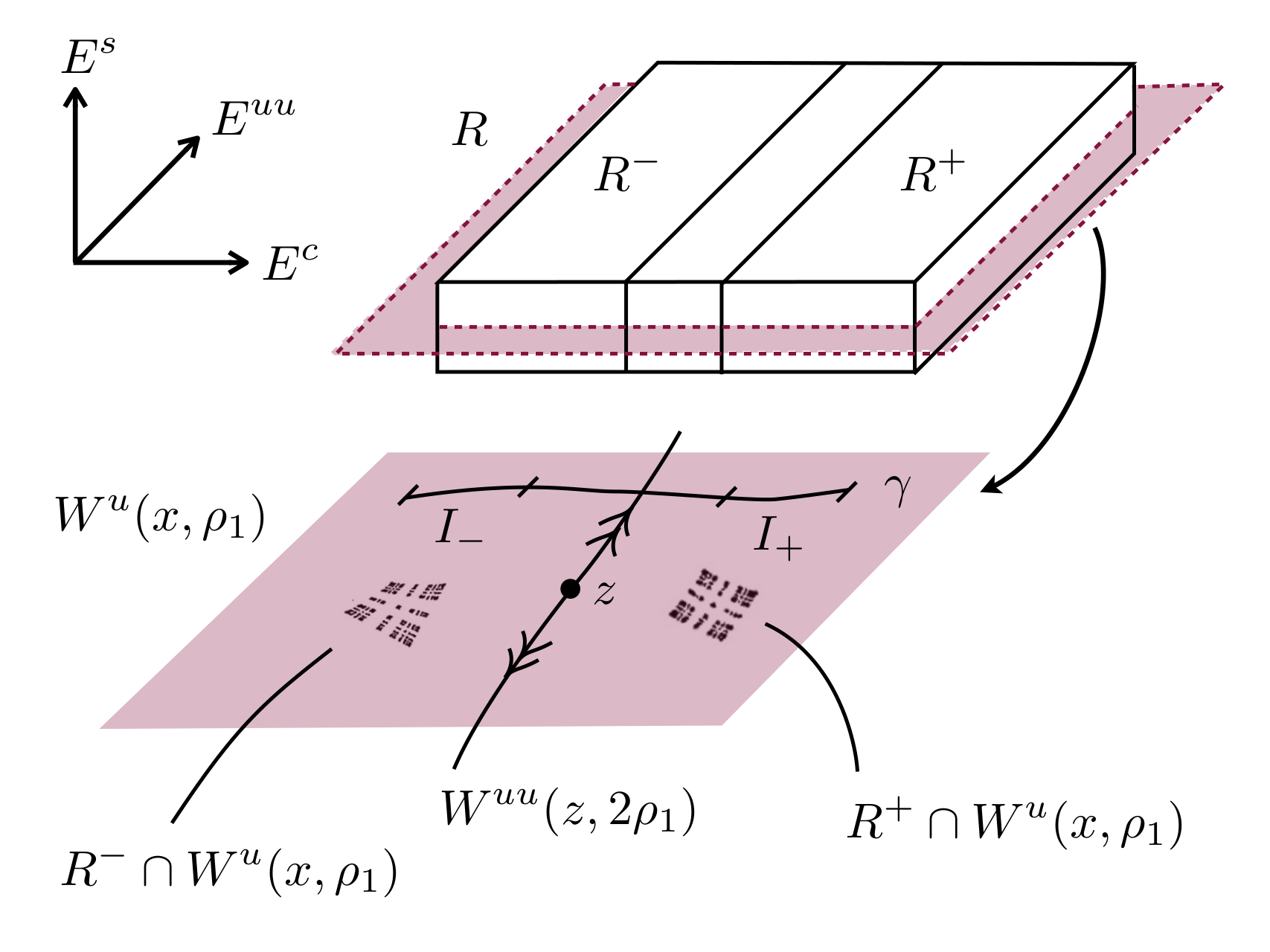
The next result says that one can extract subhorseshoes with large period and with a split Markov partition.
Proposition 6.6.
For any diffeomorphism and any horseshoe satisfying (H), for any , there exists a horseshoe endowed with a split Markov partition whose rectangles have diameter smaller than and such that the following property holds.
For every , there exist and a horseshoe such that:
- •
admits a decomposition into compact subsets
- •
the topological entropy is larger than ,
- •
for each and , the disintegration of the measure of maximal entropy of along the unstable leaves gives the same weight to and .
Proof.
Consider a Markov partition of into disjoint compact rectangles with diameter smaller than . We can furthermore require that the maximal invariant set in the smaller collection has entropy larger than . A word in is admissible if .
Fix some point . Since is essential, there exist such that are disjoint. For let
denote the itinerary of and in the partition . If is large enough, the rectangles
are small neighborhoods of in . The union is a split rectangle. Note that one can modify and take so that .
We then consider some integer large and the admissible words of length of the form or with admissible words in of length . The bi-infinite words obtained by concatenation of these words define the horseshoe . There exists arbitrarily large such that the entropy of is arbitrarily close to the entropy of , and hence is larger than .
If has been chosen large enough, we note that is disjoint from its first iterates. Hence, any segment of orbit of of length meets at one point exactly. One can thus define a Markov partition by taking rectangles of the form
with varying between and . These rectangles are compact, disjoint and naturally split by . We thus get a collection of disjoint split rectangles of . Both partitions and are Markov by construction.
Since , the set of itineraries of the forward orbits from and are equal after time . This implies that the disintegration of the maximal entropy measure of gives the same weight to and for each . Similarly, it gives the same weight to and for each .
Fix a Markov rectangle that meets after iterates: if is large enough, the set of points of whose orbit does not intersect has entropy larger than . For large (and a multiple of ), the subhorseshoe corresponds to itineraries that visit exactly every -iterates. Since is large, the entropy of is larger than . This horseshoe is -periodic: setting , it can be decomposed as
Again by symmetry of the construction the disintegration of the maximal entropy measure on gives the same weight to and for each and each . This gives the proposition. ∎
6.2.3. Proof of the reverse doubling property
Proof of Theorem 6.4.
Since there is a dominated splitting between and , there exists a thin cone field defined on a small neighborhood of and containing the bundle such that for any , and any small -curve in containing and tangent to , the backward iterates are still tangent to . By a classical distortion argument, since is uniformly contracted by backward iterations, and since is , there exists some uniform constant such that for any unit vectors tangent to at points we have
Let’s apply Proposition 6.6 to , , and a small constant : we obtain a split Markov partition of . For each and each , there exists a small curve tangent to and two disjoint compact intervals such that for any the strong manifold intersects at a point of if and at a point of otherwise. (See Figure 3.) If is small, the curve is also small.
There exist two constants , which do not depend on or on , such that:
- •
the length of is smaller than ,
- •
the distance between and in is larger than .
Choose constants small. For any a horseshoe given by Proposition 6.6, we have to prove the reverse doubling property for these constants.
We fix and . For each we consider the sequence such that for each and then define the domain
it splits in two pieces . We also consider , the largest domain contained in , and , the corresponding domains . Note that if has been chosen small, then is large.
Next choose associated to and as above. From the domination between and , the domains and are contained in the unions
| (9) |
The diameter of the strong unstable disk is much smaller than the length of the curves , . Hence the domains , are strips that are very thin in the strong unstable direction.
From the distortion estimate, the distance between and is larger than
The holonomy along the strong-unstable foliation between central curves inside the unstable plaques is uniformly Lipschitz. As a consequence there exists a uniform constant such that if are central curves associated to the domains and , then we have
| (10) |
By maximality of , the length of the associated curve is thus larger than . It follows that the distance between and is larger than .
If is chosen smaller than , then only one domain or can intersect . Since has constant Jacobian along the unstable leaves for the measure , both preimages have the same -measure. This proves that
By construction the domains for are disjoint or equal. We thus obtain a finite family such that the domain , are pairwise disjoint, and their union contains and is contained in . This proves that
This gives the desired estimate. ∎
6.3. Extraction of sparse horseshoes and proof of Theorem B
We first prove the existence of a subhorseshoe with large entropy and nice geometry.
Theorem 6.7 (Sparse subhorseshoe).
For any diffeomorphism , any horseshoe satisfying (H), and any , there exist with the following property.
For any there exist compact subsets such that
- •
each has diameter in and meet ;
- •
the neighborhoods of size of the are pairwise disjoint and homeomorphic to balls;
- •
the entropy of the restriction of to the maximal invariant set in is larger than .
The proof of this theorem is postponed until Section 6.5
Proof of Theorem B from Theorem 6.7.
Theorem B will be proved in several steps: we will first show that admits an extracted horseshoe that can be locally linearized; we then show that this subhorseshoe admits a dominated decomposition into one-dimensional subbundles and a global chart where these bundles are constants. At last we prove that after another extraction there is a subhorseshoe which is globally linear.
Fix . Note that by Theorem 3.2, we can perform if necessary an arbitrarily -small perturbation and replace by a subhorseshoe whose topological entropy is arbitrarily close to the initial entropy in order to ensure that has a dominated splitting into one dimensional subbundles.
One can by a small -perturbation replace by a diffeomorphism that is in a small neighborhood of . This is more delicate in the conservative setting: one uses [Z] for symplectic diffeomorphisms, [DM] for volume preserving ones in the case and [Av, Theorem 5] for volume preserving ones in the case .
By an arbitrarily -small perturbation we can also assume that is essential, so that the property (H) holds. Indeed if are two periodic points close in , it is possible to break the intersection between the local stable manifold of and the local strong unstable manifold of (tangent to ); the intersection between and belongs to , proving that is not contained in .
Now apply Theorem 6.7, using : we obtain . We also fix a global chart from a neighborhood of , so that we can work in ; if one considers a volume or a symplectic form, one can take it to be constant in the chart. For that will be chosen small enough, we get a family of compact sets with diameter in which meet and we introduce for each its -neighborhood and its - neighborhood . The sets are pairwise disjoint, have a diameter smaller than and contains the -neighborhood of .
For each , we choose a linear map in close to the for . We will perturb in the sets with the following lemma.
Lemma 6.8 (Local linearization).
For any and any , there exists with the following property. Consider:
- •
a compact set of the unit ball which is homeomorphic to a ball and has diameter equal to ,
- •
a -map which is a diffeomorphism onto its image and satisfies ,
then, there exists a -map which is a diffeomorphism onto its image and:
- •
coincides with outside the -neighborhood of ,
- •
coincides with a translation in ,
- •
satisfies everywhere.
If preserves the standard symplectic form or if preserves the standard Lebesgue volume and satisfies , then can be chosen to preserve it as well.
Proof.
Note that it is enough to prove the lemma for functions such that , hence that are -close to the identity. Let us fix and a compact set which is homeomorphic to a ball and has diameter equal to . One chooses two disjoint, closed connected neighborhoods of and respectively.
We consider a smooth map that coincides with on and with on .
For any -map which is a diffeomorphism onto its image, one defines . Since , if is close to the identity, is a diffeomorphism onto its image and everywhere. It coincides with on and with the identity on , hence satisfies the conclusions of the lemma.
When preserves Lebesgue, and is small, one builds a first diffeomorphism as before, which is -close to the identity. In particular the volume form is -close to the standard Lebesgue volume and coincides with it on and on . By applying [Mo], one obtains a conservative diffeomorphism of which sends on . Consequently the diffeomorphism preserves the volume. Since is obtained by integration of the form , one can check that is a translation on each connected component of and can be chosen to coincide with the identity outside . Since and are -close, is small, hence is -close to the identity as well. Since is contained in a connected component of , the diffeomorphism is a translation on by construction.
In the symplectic case, is built in a different way. The diffeomorphism is obtained from a generating function that is -close to the generating function of the identity (since is -close to the identity). The map can be obtained from the generating function .
Note that the triple is still valid for any connected compact set that is Hausdorff close to . Since the set of compact subsets of whose diameter is equal to is compact in the Hausdorff topology, there exists which is valid for all compact sets with diameter equal to . ∎
Lemma 6.8 may be restated as follows.
Corollary 6.9.
For any -diffeomorphism of the ball , and any , there exists with the following property.
For any compact set homeomorphic to the ball and with diameter smaller than , for any such that for some , there exists and a -diffeomorphism which:
- •
coincides with outside the -neighborhood of ,
- •
coincides with in ,
- •
satisfies everywhere.
If and preserve a given volume or symplectic form, then can be chosen to preserve it as well.
Proof.
It is enough to apply the previous lemma to the diffeomorphism , where belongs to and . If have been chosen small enough, is close to the identity for .
When preserves a given volume or symplectic form, one can change the coordinates so that the volume or the symplectic form coincide with the standard ones. Moreover one notices that uniformly converges to on when the diameter goes to . The previous lemma can thus still be apply in these settings provided is small enough. ∎
Applying the previous corollary independently for each provides us with a diffeomorphism which coincides with an affine map on each and with outside the union of the . The tangent maps of and are -close, and since the size of the connected components of the support of the perturbation is smaller than , the distance between and is also small. Consequently belongs to the neighborhood of . Moreover if preserves a volume or a symplectic form, by choosing the linear maps to be conservative, the perturbation still preserves the form and is locally affine in the union .
Consider a transitive hyperbolic set with entropy larger than and contained in as given by Theorem 6.7. Since and are -close in the topology, the shadowing lemma implies that the hyperbolic continuation of for is contained in the -neighborhood of , where is arbitrarily close to if the distance between and is chosen small enough. In particular, is contained in the union , hence is locally affine. Moreover has entropy larger than . By Theorem 3.3, there exists a horseshoe with entropy larger than contained in , hence locally affine as required. This gives the first part of Theorem B .
We now explain how to modify the previous construction so that the splitting is locally constant. We first introduce a family of disjoint open sets which cover and have small diameters. We choose a point in each of them. The sets given by Theorem 6.7 are only chosen after, with diameter small enough so that each set and each image is contained in one of the sets . We linearize in each domain as before but require that coincide on with the affine map where , such that
- •
and are defined by the conditions and ,
- •
the linear maps is close to the identity and sends the splitting to the splitting .
When preserves the volume or the symplectic form, we choose to preserve it as well. In the symplectic case this is possible since the two planes of the form are pairwise symplectic-orthogonal (see [BV1]).
The end of the construction is unchanged. After perturbation, the dominated splitting on for the map , coincides in each set with and hence is locally constant.
At this step we have reduced the proof of Theorem B to the case of a local diffeomorphism of a hyperbolic set in a subset of , such that is locally affine on , and the splitting of into the coordinates axes is -invariant. In the conservative case, the volume, or the symplectic form is chosen to coincide with the standard Lebesgue volume of or with the standard symplectic form of . It remains to prove that after a new extraction and a new perturbation, the linear part can be made constant.
Choose a Markov partition of into small disjoint rectangles . Since the are small, the diffeomorphism is affine on a neighborhood of : there exists a linear map such that the diffeomorphism has the form . Since the coordinates axes are preserved, is diagonal with diagonal coefficients .
For large enough, consider the sub-horseshoe of points of which visit exactly every iterates: its topological entropy is larger than . Moreover the return map on decomposes into branches labelled by compatible itineraries in , which are affine. Each itinerary is associated to a diagonal matrix whose coefficients are sums of numbers chosen among , with and . The number of such matrices grows at most polynomially in . On the other hand, the number of itineraries of length starting in grows faster than .
It follows from the pigeonhole principle that there exists a diagonal matrix and a set containing at least itineraries of length which start in and which all have the same associated diagonal matrix . The set of points in whose orbit follows these itineraries is a sub horseshoe whose topological entropy is larger than as required. It may be decomposed as a disjoint union of compact sets: . The diffeomorphism on is affine with the constant linear part .
Now cover by small disjoint open sets is such a way that is affine on each , with and , and has a linear part . We change the chart on each set by the composition of with a translation. For this new chart, the diffeomorphism has the form near each point . This completes the proof of Theorem B . ∎
6.4. Cube families
In this subsection and the following ones we prove Theorem 6.7. We thus consider a diffeomorphism and a horseshoe satisfying (H). We describe some preliminary constructions.
6.4.1. The affine chart - the scale - the metric on .
For each point , we will use smooth charts from a neighborhood of in to whose derivative at sends the splitting to the splitting
| (11) |
Since the angle between the spaces , , is bounded away from zero, one can assume that the -norm of the charts is uniformly bounded by some .
In the case preserves a volume or a symplectic form , we may assume that (resp. ) is the standard symplectic form on . Indeed, for the volume preserving case one uses [DM]. In the symplectic case, we first use Darboux’s theorem in order to rectify the symplectic form. By [BV1], the horseshoe admits a finer dominated splitting into Lagrangian subbundles
such that , , and . The subspaces and are symplectic orthogonal. All this implies that the splitting may be sent by a bounded symplectic linear map to the standard splitting (11).
Since is totally disconnected, for any scale there exist a neighborhood of having finitely many connected components , each of them has diameter smaller than , contains a point , and is included in the domain of the chart . We may also assume that the images are pairwise disjoint, so that the map which coincides with on is also a chart.
Two metrics appear: the initial metric on and the chart metric induced by from the standard metric in . At this stage, the chart depends on and has not been fixed. However the initial and charts metrics are comparable up to the constant which does not depend on . In the following we will mainly consider the chart metric.
6.4.2. First extraction - the Lyapunov exponents - the split Markov partition.
Replacing if necessary by a subhorseshoe whose entropy is arbitrarily close to the entropy of the initial horseshoe, one can assume that:
- •
(Theorem 3.3.) There exist constants such that for any invariant probability measure on the Lyapunov exponents along , , and belong to , and respectively.
One chooses large enough so that for any , if is a unit vector in , or , then belongs to the corresponding interval.
- •
(Proposition 6.6.) For any , there are subhorseshoes that are disjoint unions of the form with and entropy larger than , and there exists a split Markov partition whose rectangles have a small diameter and such that gives the same weight to and inside each unstable plaque.
6.4.3. Sheared cubes - the shear - the scale .
Let , , be orthonormal bases for the three factors of the decomposition (11). For a shear we define the linear transformation by if , if and
We denote by the image of the unit parallelepiped centered at :
The reason we need a shear will appear in Lemmas 6.11 and 6.13.
The unstable faces are the faces of spanned by the same vectors as , but one among . The other faces are the stable faces and are spanned by the same vectors as , but one among . The unstable boundary (resp. stable boundary) is the union of the unstable (resp. stable) faces.
Fix . For and at distance less than from , we define the (sheared) cube (see Figure 4)
The point is called the center of the cube and is its diameter. For any cube with center and diameter , and any , we denote by the cube centered at of diameter . The stable and unstable boundaries of are defined analogously to the boundaries of .
For , we define linear transformations by , , and . For , we define the stable and unstable -boundaries of as follows:
This partitions into and . Note also that .
Each cube has a set of unstable neighbor cubes of cardinality . The set consists of the cubes of diameter and shear that are produced from by a translation by
where each is taken in (see Figure 5).

If is small, then the local unstable manifolds are -close to planes spanned by , so that if , then the local unstable manifold does not meet the stable boundary of the , and
Choose large. We construct the cube family (at scale with shear ) as the collection:
6.4.4. Cube transitions - the boundary size .
Fix some close to . For , we say that there is a transition from to (which we denote by ) if intersects , whereas and are empty (see Figure 6).
In the following, we consider the disintegration of the measure of maximal entropy of a horseshoe along the unstable manifolds. We then define the measure induced by on the plaque for each . We will reduce the proof of Theorem 6.7 to the following proposition, which is proved in Section 6.6.
Proposition 6.10.
Consider and as introduced in Section 6.4.2.
For all , there exist and a chart with , such that if is a subhorseshoe associated to an integer and if denotes the measure induced on by the disintegration of its measure of maximal entropy along the unstable leaves, then the following holds.
There exists such that for all , any cube in the family of the chart and any point , we have:
6.5. Proof of Theorem 6.7 from Proposition 6.10
Consider a horseshoe as in the assumptions of Theorem 6.7 and . Fix a Markov partition of such that any point is uniquely determined by its itinerary in the collection of rectangles .
Proposition 6.10 applied with this value of provides us with a chart satisfying , with a boundary size and a shear . We also obtain an arbitrarily large integer and a subhorseshoe such that and which decomposes as a disjoint union .
The initial and chart metrics are equivalent up to a uniform constant. One can thus end the proof with the initial metric on . We will choose such that for any cube in a family , the -neighborhood of the cube is contained in . There exists also such that for any large and any two cubes , the quantity is bounded by . In this way, for any sufficiently small, we can choose large such that the cubes have diameter in . Note also that all points in the same cube have the same itinerary during iterates with respect to the Markov partition. Let be the collection of cubes for that meet and let denote the -neighborhood. If has been chosen sufficiently small, then the sets for and are pairwise disjoint.
Let be the union of the cubes , and let . Fix any point and such that . Since has full support, we have
Note that if there is a transition then for any point belonging to we have and moreover, the non-empty connected set is contained in . Since has constant Jacobian along the unstable leaves for the measures , by applying inductively the proposition we obtain that for each ,
Hence
Integrating over the different plaques with , there exists uniform in such that the measure of maximal entropy on satisfies:
| (12) |
Since is the Gibbs state for the potential on , the measure of points that follow a fixed itinerary of length (with respect to the Markov partition) is smaller than for some uniform in , see [Bow]. Using (12), we deduce that the number of different itineraries of length starting from and contained in is larger than . Passing to the limit as goes to proves that the topological entropy of the maximal invariant set in is larger than , hence larger than .
We have proved that, for each , there is a decomposition such that the conclusion of the theorem holds for the horseshoe and the diffeomorphism . Since are pairewise disjoint, the conclusion holds also for and by reducing : considering a family of connected cubes with small diameter associated to and , one gets a family , , , which satisfies the required properties for and . This completes the proof of Theorem 6.7.
6.6. Proof of Proposition 6.10
The proof uses the chart metric. Consider any horseshoe with larger than some , a chart whose connected components have diameter smaller than some , a cube and any .
We say that a cube is s-bad (with respect to the image ) if its stable boundary intersects (see Figure 6).
We will assume that the images of the unstable -boundaries is larger than the size of the cubes:
| (13) |
Any cube that intersects satisfies one of the following cases:
- •
either there exists a transition ,
- •
or is s-bad.
(See Figure 7.) Indeed has size and by (13) cannot intersect , which is at distance larger than from .

In the following the main point is to bound the measure of s-bad cubes that intersect
6.6.1. Measure of cube boundaries.
For the particular geometry of the cubes that we’ve defined, the reverse doubling inequality (8) can be improved.
Lemma 6.11.
For every , there is such that for any the following property holds if is sufficiently small.
For any , any and any cube such that and intersect, the measure induced on by the disintegration of the measure of maximal entropy of satisfies:
Proof.
The proof is similar to that of Theorem 6.4. We first introduce for each point and each the domains and as intersections of the -th backward image of rectangles or with the unstable plaque of .
Sublemma 6.12.
For every , there exists such that for any the following property holds if is sufficiently small.
For any , any cube and any , it holds that any point in belongs to some preimage such that:
- (1)
, and
- (2)
or is contained in a cube with .
Proof.
Assuming that is small enough, the bundles , , (viewed in the charts) are -close to constant bundles and the unstable plaques are -close to affine spaces. The sets are inside the unstable plaque of , which is stretched along a central curve and very thin in the strong unstable direction (see (9)).
Since , the plaque intersects any along its unstable boundary. The intersection with each unstable face of is transverse. It follows that the set is a union of thickened hypersurfaces of the unstable plaque of whose width along the central direction belongs to .
By (10), for any , one can consider a domain associated to a central curve of length contained in (using the constants introduced in the proof of Theorem 6.4). The two domains and are associated to subintervals whose -th preimages are separated by , which is larger than . It follows that only one domain or can intersect each thickened hypersurface . By the definition of split Markov partition, either or must contain both and . We thus deduce that in the family , …, there exists a domain such that either or is disjoint from the thickened hypersurfaces , and hence is contained in a cube with .
By (10), the larger domain is associated to a curve whose length is smaller than . It is thus contained in , provided is chosen so that
∎
For as in the previous sublemma, any point belongs to a maximal set satisfying conditions 1 and 2. In particular, the domains are disjoint or equal, they cover , and they satisfy
We obtain that
Applying the sublemma inductively, we construct a sequence such that and
for . Thus for , we have:
which implies the conclusion of Lemma 6.11. ∎
6.6.2. Localization of s-bad cubes.
In order to control the image of a cube, we require that it be smaller than (and contained in the domain of the chart ):
| (14) |
and that its diameter (in the chart) along the coordinate space be less than :
| (15) |
We define a strong unstable strip of an unstable plaque , , as the region bounded by two strong unstable leaves , with : this is the set of points that belong to a central curve in joining to .
Fix a continuous central cone field, that is, at each point close to a cone in that is a small neighborhood of . The distance between two different -leaves in is the infimum of the length of curves joining the two leaves and tangent to the central cone field. This allows us to define the width of a strong unstable strip and the distance between two strong unstable strips. Note that the strong unstable manifolds form a subfoliation of any unstable manifold , so if is small and the central cones are thin, the length of the central curves differ by a multiplicative constant, which we could take to be as close to as we want.
The next statement asserts that s-bad cubes are contained in a union of strips (see Figure 3) that are well separated by a distance and all have the same width where is chosen small, but large enough relative to so that that the following condition is satisfied:
| (16) |
Lemma 6.13.
For any , satisfying (15) and (16), and such that , the following property holds if is sufficiently small.
For any , choose satisfying (14). For any , and any , there exist strong unstable strips in and such that:
- •
each strip has width less than ;
- •
the distance between two strips is greater than ;
- •
the intersection of each s-bad cube with is contained in the union of the strips .
Proof.
By (14), the image has diameter smaller than , and the projection of on the space (inside the chart ) has diameter less than . In particular, for any point , there exist such that belongs to and has norm less than . It follows that the s-bad cubes that intersect the plaque are a subset of those satisfying:
In the charts, the plaque is close to a plane parallel to . The intersection is contained in a finite union of hyperplanes parallel to in . By projecting these hyperplanes on the -axis, one obtains a set of points that is contained in the translates of (at most) points under . One can thus project to a subset of of cardinality and then apply the following elementary lemma with .
Sublemma 6.14.
Let be a finite subset of the circle and . Then for every , there exists and a collection of open intervals with the following properties:
- •
;
- •
, for ;
- •
the length of the connected components of is larger than .
Proof.
The proof is by induction on . The cases and are easy. For , let us set . If the minimum distance between distinct points in is at least , then we put an interval of diameter centered at each point of and the conclusion holds.
Otherwise we collapse all the connected components of of length less or equal to . (There are at most many such components.) We get a circle of length with at most points. Rescaling the quotient circle to unit length and applying the inductive hypothesis with , we obtain a collection of intervals of length and separated by intervals of length larger than .
Pulling back the intervals to the initial circle, we obtain intervals of length where is the sum of the lengths of the intervals contained in that have been collapsed. One can enlarge the intervals and get intervals of length and separated by distances larger than .
By definition, . Using , , and the definitions of , and , one gets easily .
In order to check that the intervals are separated by , we estimate
| (17) |
The induction assumption gives and together with the definitions of and we get:
On the other hand, is smaller than , since . It follows that (17) is positive, which concludes the proof. ∎
From the Sublemma 6.14 we obtain and some subintervals of the circle. Pulling back the intervals to the -axis, one can extract a finite collection of intervals of length , separated by and whose union contains .
Consider the intersection (see Figure 9). On the one hand, since , it contains the intersection of with the s-bad cubes for . On the other hand, is contained in the -neighborhood of , hence in strips of of width smaller than (since by our choice of we have ) and separated by . We obtain the strips by projection of the strips of to the plaque and set : the strips are separated by a distance larger than and have width smaller than , which is smaller than by our choice of . We deduce the estimates on from the bounds on . ∎
We then cover the strips obtained from Lemma 6.13 by a collection of unstable -boundaries of cubes of size (see Figure 10). We require the cubes to be smaller than the unstable -boundary of the image cube :
| (18) |
Corollary 6.15.
In the setting of Lemma 6.13, assume that (18) holds. Then there exists a collection of cubes such that:
- (1)
each cube is disjoint from ;
- (2)
each set is non-empty and contained in ;
- (3)
;
- (4)
if intersects , then ;
- (5)
the interiors of the cubes are pairwise disjoint;
- (6)
the inner cubes and the strips do not intersect.

Proof.
For each strip , we choose a point in and (in the chart ) we consider the cubes of the form
that either intersect the strip or that have an unstable neighbor cube that intersects this strip. By construction, the union of these cubes contains .
By the inequality (18), the size of the cubes is much smaller than the distance between and in the plaque . This implies item (1). Moreover the intersection of each cube with is contained in .
Recall that is -close to a plane spanned by and has width smaller than . Note also that belongs to the center of an unstable face of some adjacent cubes . Any cube that intersects is the image of or by a translation by a bounded vector in : it also intersects near the center of an unstable face. The other cubes are unstable neighbor cubes of those who intersect . In particular, item (2) holds. Since the width of is smaller than , we deduce that the inner cubes do not intersect the strip .
The collection is the union of the collection of cubes associated to each strip . Since the distance between the strips is larger than , the cubes associated to do not intersect the cubes associated to if . The other items follow. ∎
6.6.3. End of the proof of Proposition 6.10
Given , we make the following choices:
Lemma 6.16.
Under these assumptions, the union of the s-bad cubes in that intersect has measure smaller than
Proof.
By Lemma 6.13, and (13) (the size of the cube in is much smaller than the unstable -boundary of ), we aim to bound the -measure of
By Corollary 6.15, items (3) and (6), it is bounded by:
By Lemma 6.11, the measure of the -boundary of each is smaller than
If , then the cubes still belong to the family (by Corollary 6.15 item 4); moreover each cube belongs to no more than sets . This gives
Consider any cube that intersects and take . Then we claim that and . Indeed:
- •
, since from and (16) the size of the cubes in is smaller than the -boundary size of the cubes .
- •
- •
and intersect: since intersects , is not an s-bad cube, and since , the inner cube and intersect; this implies that the unstable neighbor cube also intersect .
- •
- •
Applying Lemma 6.11 to the cubes that intersect it follows that
where is the family of cubes such that and whose intersection with is non-empty and contained in .
We now bound the measure:
where is the collection of that intersect .
The last sum may be decomposed in three parts:
- (1)
We first consider the cubes that are s-bad: Lemma 6.16 implies
- (2)
We then consider the inner part of the cubes that are not s-bad. As explained at the beginning of Section 6.6 we necessarily have .
- (3)
We finally consider the boundary part of the cubes that are not s-bad. Since , Lemma 6.11 applies and gives
Note that a cube appears at most times in the last sum. Moreover since it is an unstable neighbor of a cube that is not s-bad and intersects , the cube must also intersect . One may thus again distinguish those that are s-bad, where we use Lemma 6.16, from those that are not s-bad and satisfy . This gives:
Combining these estimates gives:
By our choice of we have . One gets the estimate of Proposition 6.10 since has a constant Jacobian along the unstable leaves for the measure .
7. Birth of blenders inside large horseshoes
In this section we prove Theorem C.
7.1. The recurrent compact criterion for horseshoes
Let be a horseshoe for a diffeomorphism whose unstable bundle has a dominated splitting . Let be the strong unstable, unstable and stable dimensions and let the dimension of the bundle .
The local strong unstable lamination . For any that is -close to and any in the continuation , there exist local unstable manifolds , which depend continuously on in the topology and which satisfy
Each local unstable manifold supports a strong unstable foliation tangent to and for each we denote by the (connected) leaf containing . The collection of all local strong unstable leaves defines the local strong unstable lamination associated to . Since is totally disconnected we may assume furthermore that for any the plaques are either disjoint or equal.
The transversal . We then consider a submanifold such that for each , the intersection between the closures of and is contained in , is transverse to the strong unstable foliation and contains at most one point of each strong unstable leaf. In particular these properties still hold for and the local strong unstable lamination if is -close to .
The following definition comes from [MS] and generalizes a property introduced in [MY] for producing robust intersections of regular Cantor sets.
Definition 7.1.
A compact set is recurrent (with respect to ) if for any points and , there exists , and some point contained in the interior of (in the topology of ), such that and .
This property is robust and implies that is a -stable blender, as stated in the two next propositions (which also come from [MS]):
Proposition 7.2.
The compact set is still recurrent with respect to the strong unstable leaves for the diffeomorphisms that are -close to .
Proof.
Consider the (closed) set : it is contained in a small neighborhood of if is -close to . For any , consider with and such that and . Then for any that is -close to and any that is close to , one can consider that is close to such that . Since belongs to , by continuity there exists such that . By compactness, there exists a small neighborhood of such that this property holds for any for any . ∎
Proposition 7.3 (Recurrent compact criterion).
Consider a horseshoe with a strong unstable bundle of codimension . If admits a recurrent compact set (with respect to ) which intersects at least one plaque then it is a -stable blender.
Proof.
We start with preliminary considerations:
- (1)
By compactness, the integer in Definition 7.1 may be chosen to be bounded by some .
- (2)
Changing the metric, we may assume that at each point of . Iterating backwards, we may also assume that the local unstable manifolds are arbitrarily small. Since is totally disconnected, there exists a smooth foliation in a neighborhood whose leaves have tangent spaces close to the bundle . This defines local projections onto local unstable manifolds.
- (3)
The dominated splitting gives the existence of an invariant cone field : for each in a neighborhood of , the cone is open in , and . Moreover, contains and is transverse to . Replacing the cone field by a forward iterate, we obtain an arbitrarily thin cone field around the bundle and defined on a neighborhood of the lamination . For any that is -close to , the cone field is still invariant.
Let be a submanifold -close to a local strong unstable manifold where and . More precisely, this means that there exists a small constant such that is tangent to , its distance to (measured along the leaves of ) is smaller than and its projection to contains a point -close to .
Claim.
Let be a diffeomorphism -close to . Assume that is close to the local strong unstable manifold where and . Consider , , and such that . Then contains an open submanifold -close to , for some .
Proof.
Since and is bounded, there exists whose closure is close to in the Hausdorff topology. From (3), it is tangent to the cone field and from (2), its distance to is smaller than . The projection of to intersects at a point close to . Since belongs to the interior of , the point belongs to also. Consequently is -close to and the claim is proved. ∎
Now consider and as in the claim. Applying the claim inductively, we get a decreasing sequence of submanifolds and an increasing sequence of integers such that each is close to a local strong unstable manifold. This proves that the forward orbit of the point remains in a small neighborhood of . Consequently, belongs to the intersection of and a local stable manifold of a point of . This proves that is a -blender. ∎
7.2. The recurrent compact criterion for affine horseshoes
Let , . We now assume that satisfies the following additional property.
Definition 7.4.
We say that is a standard affine horseshoe if there exist:
- •
a chart with ,
- •
a linear map which is a product where and are contractions of and ,
- •
pairwise disjoint translated copies ,…, of in ,
- •
pairwise disjoint translated copies ,…, of in ,
with the following properties:
- •
sends to for each ,
- •
agrees on with the map , for some , and
- •
is the maximal invariant set in .
Note that, denoting , the cubes are the connected components of that intersect . See Figure 11.
We will assume furthermore that is partially hyperbolic: preserves the dominated splitting , where . In particular, and are products , and each is a product where and is the projection onto the center coordinate. We thus obtain a family of affine contractions , , which send to respectively and coincide with . This defines a (finitely generated) iterated function system (IFS) in .
Denoting , we have that each strong unstable plaque with can intersect at most distinct rectangles . This remark applied to any iterate shows that for any point ,
| (19) |
We state a definition for IFS which is the analogue of Definition 7.1.
Definition 7.5.
The IFS satisfies the recurrent compact condition if there exists a nonempty compact set such that for every there exist and with .
Proposition 7.6.
If the central IFS associated to a partially hyperbolic standard affine horseshoe as above satisfies the recurrent compact condition, then admits a recurrent compact set.
Proof.
We introduce the local strong unstable lamination by plaques of the form where . We then define the section and introduce the compact set .
Let us consider in and a point in . We have , hence there exists and with . Since intersects , there exists a point of the form such that belongs to . The point has the property that . Moreover since belongs to , the point belongs to as required. ∎
7.3. Perturbations of iterated function systems
Let , let be a linear contraction, and write . For , let such that the affine contractions send into its interior. For any finite word in let . For large enough, we consider the IFS .
We will assume furthermore that there exists and such that:
- •
,
- •
for any and .
For we define and consider the space of functions that satisfy each time the last letters of and coincide. Since can be identified with it is a probability space (endowed with the product Lebesgue measure).
The following probabilistic argument allows us to perturb the initial iterated function system so that the recurrent compact condition is satisfied.
Proposition 7.7.
Under the previous assumptions, if is large enough, then there exists such that the IFS induced by the affine contractions
satisfies the recurrent compact condition.
Proof.
Let .
Claim.
There exists a compact set with Lebesgue measure of points that belong to a least images associated to sequences whose last letters are different.
Proof.
Let be the set of points that belong to at least images where . By our assumptions, a point can belong to at most such images (here we apply the estimate (19) to the point ). Considering the images of by all possible maps , one gets:
This gives .
Fix in and some . The number of images containing and whose last letters of coincide with is equal to the number of images with which contain . It is thus smaller than . It follows that the points belong to at least images associated to sequences whose last letters are different. ∎
Consider the tiles , where , and their cores . We denote by the union of the tiles which intersect and by the union of the cores of these tiles. We have . Finally, we define
Then the conclusion of the proposition holds for any parameter such that:
| (20) |
For a fixed , we estimate the measure of the set of parameters
| (21) |
Pick some which belongs to a same tile as . For each such that , the probability that is
The point belongs to at least images associated to words whose last letters are pairwise different. For these different words , the events are independant in the parameter space . Consequently, the probability of the event (21) is at most . From the definition of and , this gives:
By our choice of , we have . Since the cardinality of grows at most exponentially with , it follows that the measure of the set
becomes arbitrarily small. In particular, for large there exists such that condition (20) holds. Hence the result follows. ∎
7.4. Reduction to standard affine horseshoes
Any affine horseshoe contains large standard horseshoes (Definition 7.4). Note that the condition (4) can be preserved by this construction.
Proposition 7.8.
Consider and an affine horseshoe with constant linear part. Then for any there exist , a chart and such that
- •
and is a standard horseshoe of for the chart ,
- •
,
- •
the diameter of is smaller than ,
- •
if are the connected components of that intersect , then for each and .
Proof.
By extraction one first reduces to the case of a horseshoe whose dynamics are conjugate to a full shift. Indeed, by [An2], any horseshoe is topologically conjugate to a transitive Markov subshift over a finite alphabet , hence it is enough to work with a transitive Markov subshift and to apply the following lemma.
Lemma 7.9.
Let be a transitive Markov subshift on a finite alphabet . Then for any , there exists a compact subset and such that
- •
and for ,
- •
the restriction of to is conjugate to the shift on , and
- •
.
Proof.
Let us fix a symbol and consider for large the collection of words of length such that and appears in . Their number is larger than . Note that the set of words that can be written as for some sub word with length smaller than has cardinality smaller than . Consequently, there exists a word which does not have such a decomposition. In particular appears only twice as a sub-word of .
The number of different subwords of length in is smaller or equal to . Consequently, there exists a collection of words which are not subwords of .
If is a large multiple of , let be the collection of words of length of the form with and for . One labels the elements of by where is larger than .
Let be the collection of sequences such that belongs to for each . We have and the restriction of to is conjugate to the shift on . By construction of and , the image intersects if and only if . ∎
From Lemma 7.9 one can now assume that the dynamics of on is conjugate to the shift on by a homeomorphism and that the entropy on the subhorseshoe obtained by deleting one symbol is larger than .
Since is affine, up to a conjugacy, we may assume that it is contained in and that is piecewise affine in a neighborhood of with a constant linear part . By an affine change of the coordinates, we may also assume that sends into its interior and that sends sends into its interior. Let denote the fixed point and let be a small cube centered at that is the pre image of the standard cube by an affine map of the form . Hence is a product .
One can find and contained in such that for . Denote by the connected component of containing : it is a cube of the plane . If has been chosen small enough, we may assume that is disjoint from for any . In the same way, denoting by the connected component of containing , we may assume that is disjoint from for any .
We now fix and consider much larger. Set . Let and . To any sequence we associate the point such that satisfies:
- •
for ,
- •
for ,
- •
for .
By construction and belong to the interior of , and the forward images of the connected component of containing (resp. the backward images of the connected component of containing ) are disjoint from the boundary of . Since is affine in a neighborhood of , this implies that the connected component of containing is a set of the form , where is contained in the interior of . Analogously, is a set of the form , where is contained in the interior of . Moreover the iterates for are disjoint from .
The rectangles (resp. ) for are pairwise disjoint. Consequently, the maximal invariant set for in is a standard horseshoe.
If is sufficiently large, then the entropy of on satisfies the required lower bound:
∎
7.5. Proof of Theorem C
We can now complete the construction of blenders for affine horseshoes with large entropy. Consider and an affine horseshoe with constant linear part that is partially hyperbolic and satisfies condition (4). Denote by and the smallest and the largest positive Lyapunov exponents of ; by (4), we can choose such that
| (22) |
| (23) |
By Proposition 7.8, we can assume that there exist , a decomposition
and a chart such that:
- •
is a standard horseshoe for in the neighborhood ,
- •
is contained in finitely many components of ,
- •
for any and , and
- •
is arbitrarily close to .
Consequently from (23) we have:
| (24) |
As explained in Section 7.2, the standard horseshoe of defines an IFS inside the center space with affine contractions of the form , . Moreover coincides with and if we set , then the property (19) holds and (24) gives .
We can thus apply Proposition 7.7 and find large and a function such that, setting , we have:
- •
the IFS induced by the affine contractions
satisfies the recurrent compact condition,
- •
we have each time the last letters of and coincide.
After conjugating in the chart , the horseshoe for is the maximal invariant set in the cube for the dynamics induced by some affine maps:
Consider the standard horseshoe for contained in and defined by the affine maps where and . Each of these maps is defined on a domain . If denotes the contraction of induced by the map , then .
We now explain how to modify on , where is a small neighborhood of . Start by fixing a word . Now consider the image ; it contains all the sets such that the last letters of coincide with . Moreover the distance from each such set to the boundary of is greater than , where is a lower bound for the distance of the sets to the complement of .
By construction, there exists that coincides with all the vectors associated to the words whose last letters coincide with . We modify inside by a diffeomorphism that coincides on each domain with
Note that
is much smaller than , and hence than the distance between the sets and the complement of , from inequality (22). Consequently diffeomorphism we obtain is -close to , provided has been chosen large enough. Repeating this construction independently in each domain , we obtain the diffeomorphism . Note that can be chosen to preserve the volume if does.
By construction, the consecutive iterates of by are disjoint. It follows that the diffeomorphism has a standard horseshoe whose IFS coincides with the affine contractions , . By Propositions 7.3 and 7.6 this horseshoe is a -stable blender. Consequently the union of the iterates , , is a -stable blender for , as required. Note also that the support of the perturbation is contained in a small neighborhood of , which has arbitrarily small diameter.
8. Appendix: Approximation of hyperbolic measures by horseshoes
We prove in this section the version of Katok’s approximation of hyperbolic measures stated in Theorem 3.3. Recall that we have fixed a diffeomorphism in , an ergodic hyperbolic measure , a constant and a neighborhood of in the weak* topology.
8.1. Uniformity blocks
Our goal is to extract a subset of that generates a horseshoe with large entropy. In order to select enough orbit types, we will need to shadow certain pseudo-orbits for by true -orbits. Such shadowing lemmas exist for nonuniformly hyperbolic dynamics, but we need one especially adapted to our setting, allowing us to control Lyapunov exponents. The orbits will be selected from points visiting a special set called a uniformity block.
We first introduce the Oseledets-Pesin charts associated to an ergodic measure. See Theorem S.3.1 in [KH].
Theorem 8.1 (Pesin).
Let be a diffeomorphism preserving the ergodic probability measure and let . Then there exist , measurable with , two measurable functions and a measurable family of invertible linear maps satisfying the following properties.
- (1)
and for any .
- (2)
If are the Lyapunov exponents of , with multiplicities , then for any there are such that
- (3)
In the charts , the maps are defined on and satisfy at every .
- (4)
For any and any ,
The sets are called regular neighborhoods of the points . They decay slowly exponentially in size (at rate at most ) along the orbits.
Definition 8.2.
A compact set with is a uniformity block for (with tolerance ) if there exist as in Theorem 8.1 with such that are continuous on .
For any tolerance , Theorem 8.1 and Lusin’s theorem imply the existence of uniformity blocks with measure arbitrarily close to .
8.2. Shadowing theorem
The shadowing theorem we will use applies to special pseudo-orbits – those with jumps in a uniformity block for a hyperbolic measure . A sequence is an -pseudo-orbit with jumps in a set if and meet for arbitrarily large and moreover
The following theorem uses the hyperbolicity assumption on the measure .
Theorem 8.3.
For any with ergodic hyperbolic measure , there exists such that, for every sufficiently small and every uniformity block for of tolerance , the following property holds for some constants .
If is an -pseudo-orbit with jumps in and , then there exists a unique whose orbit -shadows , i.e. for all . Moreover belongs to the regular neighborhood .
If shadow two pseudo-orbits , such that for , then
We will use the classical shadowing theorem for sequences of diffeomorphisms (see, e.g. [Pi]).
Theorem 8.4.
For every there exist with the following property.
Let and satisfying and for each let . Let , where , be a sequence of diffeomorphisms with and fix any .
Then every -pseudo-orbit for is -shadowed by a unique -orbit.
More precisely: for every sequence in satisfying for all , there exists a sequence in satisfying and for all . This sequence is unique: for any sequence in satisfying for all , and for any , we have:
Proof of Theorem 8.3.
Choose a positive lower bound for the . We set and get constants from Theorem 8.4. We choose . We consider a uniformity block for with tolerance and associated to functions . Assuming that is small enough, for any map and for any linear map such that , there exists a -map which coincides with on and satisfies . We extend in this way each diffeomorphism to a diffeomorphism of agreeing with on and such that .
Let be an upper bound for , . We choose such that for each . Moreover if is small enough, when are -close, the diffeomorphisms and are -close in the -topology. In particular can be extended to a diffeomorphism of that coincides with on so that .
Fix and let be a -pseudo-orbit with jumps in . We consider the sequence of diffeomorphisms of defined by if and otherwise. In the first case and in the second case . The pseudo-orbit is thus -shadowed by an orbit of .
At times such that we have by our choice of . At other times, we consider the smallest interval of containing such that . The sequence may be compared to the orbit of which coincides with for the indices . Consequently,
From the property (1) in Theorem 8.1 we have:
which implies that still holds. The projection satisfies , so that the sequence -shadows where . By construction is an orbit of .
If is another orbit that shadows a pseudo-orbit such that for , the lifts and may be compared. From Theorem 8.4,
This completes the proof of Theorem 8.3. ∎
8.3. Metric entropy
For we define the dynamical distance
For and , let denote the minimal cardinality of the families of -balls of radius whose union has measure larger than .
Theorem 8.5 (Katok, Theorem 1.1 in [Ka]).
For any ,
8.4. Proof of Theorem 3.3
We choose a and a finite collection of continuous functions on such that contains the set of probability measures satisfying:
The tolerance
Define cones of by:
where . Let small such that the shadowing theorem holds. We will consider linear maps that are -close to diagonal maps with
If is chosen sufficiently small, then for any and for any such , the closure of the cone is mapped by inside . Moreover if is the image of by , then
Symmetrically, if is the image of by then
We then choose a uniformity block for with tolerance .
The separation scale
Choose such that
Next choose a separation scale such that
and a separation time such that implies
For any time , in any subset of of -measure at least , the maximal -separated sets contain at least .
The shadowing scale and the common return time
We choose so that , where are given by Proposition 8.3 for the uniformity block .
Lemma 8.6.
There are , an -ball centered at a point in and a set such that:
- •
the points of are -separated in the distance ,
- •
,
- •
for each and ,
- •
the cardinality of is larger than .
Proof.
Cover by finitely many -balls centered at points . For , let
The Birkhoff Ergodic Theorem implies that as . Fix such that , and let be a maximal -separated set in . By our choice of , we have
For , let
and let be a value of maximizing . Then
Next choose such that has maximal cardinality, and let and . Then from the choice of and since , we get the required estimate
∎
The set
Consider the shift over the alphabet . Since the diameter of is smaller than , each is associated to the -pseudo-orbit:
which is obtained by concatenating the orbit segments of length starting at the points . Theorem 8.3 implies that for each such pseudo-orbit there is a unique point whose orbit shadows. Consequently, the union of all the orbits that shadow the elements of is an -invariant compact set. By the last property of the shadowing theorem, the map is continuous (for the natural product topology on ). Hence conjugates the shift to .
Since for distinct , there exists such that , and since , it follows that if and -shadow distinct elements of , then and are distinct as well. This implies that is a homeomorphism. We define . It is a transitive -invariant compact set. From this we will obtain the entropy estimate (conclusion (2) of Theorem 3.3):
From the construction of , for any , we have
By our choice of , if for some , we have , then
Since , it follows that if a point -shadows a pseudo-orbit in , then
From this conclusion (3) follows.
By construction is contained in the -neighborhood of the support of . Assuming that has been chosen small enough, intersects any -ball centered at points in the support of , hence is -close to the support of in the Hausdorff distance, which gives conclusion (1).
By the shadowing theorem, any orbit in stays in the regular neighborhoods of the pseudo-orbit it shadows. Moreover is contained in the regular neighborhood of the center of and is preserved by . By properties (2) and (3) in Theorem 8.1 and by the choice of the tolerance constant, it follows that after conjugacy by the chart , the derivative of preserves the cones . The cone field criterion implies that has a dominated splitting as in condition (4):
By definition and invariance of the cones, the growth of the iterates of any vector in is given by its second coordinate in . Consequently for in and large enough we obtain condition (5):
Since the exponents are all different from zero, the set is hyperbolic.
We can reduce to the case where is a horseshoe by applying the following proposition.
Proposition 8.7.
Let be a hyperbolic set for a -diffeomorphism . Then for any , there exists a horseshoe that is -close to in the Hausdorff topology and satisfies .
Proof.
The set will be obtained through the shadowing lemma after fixing a collection of pseudo-orbits. This construction ensures that is semi-conjugate to a subshift. In order to prove that is totally disconnected we need to choose these pseudo-orbits so that this semi-conjugacy is a conjugacy. This uses an argument similar to the proof of Lemma 7.9.
Let . The shadowing lemma associates arbitrarily small constants such that any -pseudo-orbit contained in is -shadowed by an orbit of . Arguing as previously, there exists arbitrarily large and a point such that contains a set of sequences satisfying:
- •
contains at least elements,
- •
each sequence is a -pseudo-orbit, and
- •
any two such sequences , are -separated: there exists such that .
We may assume that there is in such that the -periodic pseudo-orbit is shadowed by an orbit whose minimal period is exactly . Indeed the collection of periodic orbits which have same period and shadow different , are -separated. Hence the number of those whose minimal period is smaller than is at most . This is less than the total number of elements of .
Fix such a sequence . By construction the only sub-intervals of length of that are -shadowed by are the initial and the final sub-intervals.
The number of sequences that -shadow a sub-interval of length of is smaller than , by the separation assumption. Consequently, one can find a subset with such that the do not -shadow any sub-interval of length of .
We then choose large and consider pseudo-orbits of the form
such that when or and otherwise. Each of these sequences is shadowed by the orbit of a unique point. This collection of orbits is a compact set invariant by and conjugate to the shift on .
By the choice of and , two different pseudo-orbits are -separated and are -shadowed by disjoint orbits. Consequently, is disjoint from its first iterates. The invariant compact set is a hyperbolic set with entropy larger than and conjugate to a transitive subshift of finite type. By [An2], any hyperbolic set conjugate to a subshift is a horseshoe and so is a horseshoe. By construction it is arbitrarily close to in the Hausdorff topology. ∎
The proof of Theorem 3.3 is now complete.
Acknowledgements.
We thank Carlos Gustavo Moreira, Xiao-Chuan Liu and Pierre-Antoine Guihéneuf for helpful conversations and comments.
References
- [An1] D. Anosov, Geodesic flows on closed Riemannian manifolds of negative curvature. Trudy Mat. Inst. Steklov. 90 (1967).
- [An2] D. Anosov, Extension of zero-dimensional hyperbolic sets to locally maximal ones. Sb. Math. 201 (2010), no. 7-8, 935–946.
- [Av] A. Avila, On the regularization of conservative maps. Acta Math. 205 (2010), 5–18.
- [AB] A. Avila, J. Bochi, Nonuniform hyperbolicity, global dominated splittings and generic properties of volume-preserving diffeomorphisms. Trans. Amer. Math. Soc. 364 (2012), no. 6, 2883–2907.
- [ABW] A. Avila, J. Bochi, A. Wilkinson, Nonuniform center bunching and the genericity of ergodicity among partially hyperbolic symplectomorphisms. Ann. Sci. Éc. Norm. Supér. 42 (2009), 931–979.
- [ACW] A. Avila, S. Crovisier, A. Wilkinson, Diffeomorphisms with positive metric entropy. Inst. Hautes Études Sci. Publ. Math. 124 (2016), 319–347.
- [BaBo] A. Baraviera, C. Bonatti, Removing zero Lyapunov exponents. Ergodic Theory Dynam. Systems 23 (2003), no. 6, 1655–1670.
- [BCDW] C. Bonatti, S. Crovisier, L. Díaz, A. Wilkinson What is … a blender? Notices of the AMS, 63 (2016), 1175–1178.
- [BFP] J. Bochi, B. Fayad, E. Pujals, A remark on conservative diffeomorphisms. C. R. Math. Acad. Sci. Paris 342 (2006), no. 10, 763–766.
- [BV1] J. Bochi, M. Viana, Lyapunov exponents: how frequently are dynamical systems hyperbolic? Modern dynamical systems and applications 271–297, Cambridge Univ. Press, Cambridge, 2004.
- [BV2] J. Bochi, M. Viana, The Lyapunov exponents of generic volume-preserving and symplectic maps. Ann. of Math. 161 (2005), no. 3, 1423–1485.
- [BD] C. Bonatti, L. Diaz, Persistent nonhyperbolic transitive diffeomorphisms. Ann. of Math. 143 (1996), no. 2, 357–396.
- [BDP] Bonatti, C., Diaz, L, E. Pujals, A -generic dichotomy for diffeomorphisms: weak forms of hyperbolicity or infinitely many sinks or sources. Ann. of Math. 158 (2003), no. 2, 355–418.
- [BMVW] C. Bonatti, C. Matheus, M. Viana, A. Wilkinson, Abundance of stable ergodicity. Comment. Math. Helv. 79 (2004), no. 4, 753–757.
- [BGV] C. Bonatti, X. Gómez-Mont, M. Viana, Généricité d’exposants de Lyapunov non-nuls pour des produits déterministes de matrices. Ann. Inst. H. Poincaré Anal. Non Linéaire 20 (2003), no. 4, 579–624.
- [Bow] R. Bowen, Equilibrium states and the ergodic theory of Anosov diffeomorphisms. Lecture Notes in Mathematics 470. Springer-Verlag, Berlin-New York, 1975.
- [Br] M. Brin, Topological transitivity of a certain class of dynamical systems, and flows of frames on manifolds of negative curvature. Functional Anal. Appl. 9 (1975), 8–16.
- [BW] K. Burns, A. Wilkinson, On the ergodicity of partially hyperbolic systems. Ann. of Math. (2) 171 (2010), no. 1, 451–489.
- [DM] B. Dacorogna, J. Moser, On a partial differential equation involving the Jacobian determinant. Ann. Inst. H. Poincaré Anal. Non Linéaire 7 (1990), no. 1, 1–26.
- [DW] D. Dolgopyat, A. Wilkinson, Stable accessibility is dense. Geometric methods in dynamics. II. Astérisque 287 (2003), 33–60.
- [GPS] M. Grayson, C. Pugh, Charles, M. Shub, Stably ergodic diffeomorphisms. Ann. of Math. (2) 140 (1994), no. 2, 295–329.
- [H1] E. Hopf, Statistik der geodätischen Linien in Mannigfaltigkeiten negativer Krümung . Ber. Verh. Sächs. Akad. Wiss. Leipzig 91 (1939), 261–304.
- [H2] E. Hopf, Statistik der Lösungen geodätischer Probleme vom unstabilen Typus. II. Math. Ann. 117 (1940). 590–608.
- [HMY] Y. Han, D. Müller, D. Yang, A theory of Besov and Triebel-Lizorkin spaces on metric measure spaces modeled on Carnot-Carathéodory spaces. Abstr. Appl. Anal. (2008).
- [Ka] A. Katok, Lyapunov exponents, entropy and periodic orbits for diffeomorphisms. Inst. Hautes Études Sci. Publ. Math. 51 (1980), 137–173.
- [KH] A. Katok, B. Hasselblat, Introduction to the modern theory of dynamical systems. Encyclopedia of Mathematics and its Applications 54. Cambridge University Press, Cambridge, 1995.
- [Ko] A. Kolmogorov, Théorie générale des systèmes dynamiques et mécanique classique. Proceedings of the International Congress of Mathematicians (Amsterdam 1954) Vol. 1, 315–333
- [LY1] F. Ledrappier, L.S. Young, The metric entropy of diffeomorphisms. I. Characterization of measures satisfying Pesin’s entropy formula. Ann. of Math. 122 (1985), 509–539.
- [LY2] F. Ledrappier, L.S. Young, The Metric Entropy of Diffeomorphisms. II. Relations between Entropy, Exponents and Dimension. Ann. of Math. 122 (1985), 540–574.
- [MS] C.G. Moreira, W. Silva, On the geometry of horseshoes in higher dimensions. Preprint (arXiv:1210.2623).
- [MY] C.G. Moreira, J.C. Yoccoz, Stable Intersections of Regular Cantor Sets with Large Hausdorff Dimensions. Ann. of Math. (2) 154 (2001), 45–96.
- [Mo] J. Moser, On the volume elements on a manifold. Trans. Amer. Math. Soc. 120 (1965), 286–294.
- [P] Y. Pesin, Characteristic Ljapunov exponents, and smooth ergodic theory. Uspehi Mat. Nauk 32 (1977), no. 4 (196), 55-112, 287.
- [Pi] S. Yu. Pilyugin, Shadowing in Dynamical Systems, Lecture Notes Math., 1706, Springer-Verlag, Berlin, 1999.
- [PS] C. Pugh, M. Shub, Stably ergodic dynamical systems and partial hyperbolicity. J. Complexity 13 (1997), no. 1, 125–179.
- [PSW] C. Pugh, M. Shub, A. Wilkinson, Hölder foliations, revisited. J. Mod. Dyn. 6 (2012), 79–120.
- [RRTU] F. Rodriguez-Hertz, M.A. Rodriguez-Hertz, A. Tahzibi, R. Ures, New criteria for ergodicity and nonuniform hyperbolicity. Duke Math. J. 160 (2011), no. 3, 599–629.
- [RRU] F. Rodriguez-Hertz, M.A. Rodriguez-Hertz, R. Ures, Accessibility and stable ergodicity for partially hyperbolic diffeomorphisms with 1D-center bundle. Invent. Math. 172 (2008), no. 2, 353–381.
- [T2] A. Tahzibi, Stably ergodic diffeomorphisms which are not partially hyperbolic. Israel J. Math 142 (2004), 315–344.
- [Z] E. Zehnder, Note on smoothing symplectic and volume-preserving diffeomorphisms. In Geometry and Topology (Rio de Janeiro, 1976). Lecture Notes in Math. 597, 828–854.