Finite element approximation of the fields of bulk and interfacial line defects

The tensor $\mathbfit{\Pi}$ for a discrete g.disclination can be defined for prescription as given data as follows. Figure 2 shows an eigenwall field ${\mathbfit S}$ supported in a layer, whose termination represents the g.disclination core. The layer is, in general, ‘non-planar’ and its termination not a straight ‘line’. We assume the layer to be amenable to the description

$${\mathbfit s}(\xi^{1},\xi^{2},\xi^{3})={\mathbfit x}(\xi^{1},\xi^{2})+\xi^{3}\mathbfit{\nu}(\xi^{1},\xi^{2}),$$

(11)

where ${\mathbfit x}$ is the ‘mid-surface’ of the layer, parametrized by curvilinear coordinates $(\xi^{1},\xi^{2})$, and $\mathbfit{\nu}$, the unit normal field to the mid-surface, is defined as

$$\mathbfit{\nu}(\xi^{1},\xi^{2})=\frac{\frac{\partial{\mathbfit x}}{\partial\xi^{1}}\times\frac{\partial{\mathbfit x}}{\partial\xi^{2}}}{|\frac{\partial{\mathbfit x}}{\partial\xi^{1}}\times\frac{\partial{\mathbfit x}}{\partial\xi^{2}}|}.$$

(12)

$\xi^{3}$ serves as the remaining coordinate parametrizing the 3-dimensional layer. The parametrization (in the vicinity of the g.disclination core) is such that the surface $\xi^{1}=0,-\frac{t}{2}\leq\xi^{3}\leq\frac{t}{2}$ coincides with the layer termination within the body, and the surfaces $\xi^{3}=\pm\frac{t}{2}$ are the top and bottom surfaces of the layer, respectively. The layer mid-surface (and therefore the $\mathbfit{\nu}$ field), is assumed known (e.g. from observations) for the definition of the ${\mathbfit S}$ and $\mathbfit{\Pi}$ fields in this static setting. Denote the i-elastic distortion field (the inverse rotation field in the disclination case) of the upper part as ${\mathbfit W}_{1}$; the i-elastic distortion of the lower part is denoted as ${\mathbfit W}_{2}$. The thickness of the layer is $t$ in the normal direction to the layer. The eigenwall field ${\mathbfit S}$ in the layer is defined as

$${\mathbfit S}=a(\xi^{1})\dfrac{\left({\mathbfit W}_{1}-{\mathbfit W}_{2}\right)}{t}\otimes\mathbfit{\nu},$$

(13)

where $a(\xi^{1})$ is a scalar function indicating the longitudinal extent of the core of the g.disclination; a candidate we utilize is

$$a(\xi^{1})=\begin{cases}0\qquad\xi^{1}<0\\ \frac{1}{c}\xi^{1}\qquad 0\leq\xi^{1}<c\\ 1\qquad\xi^{1}\geq c,\end{cases}$$

(14)

with $c$ being the core width. The field ${\mathbfit S}$ is assumed to vanish outside the layer. In general, ${\mathbfit W}_{1}$ and ${\mathbfit W}_{2}$ could be spatially varying along the longitudinal directions of the layer, while being always uniform in the transverse direction. Here we assume that ${\mathbfit W}_{1}$ and ${\mathbfit W}_{2}$, viewed as fields in the layer, are constant (In Section 5.12.2 we encounter a curved twin boundary of a lenticular inclusion where this is not the case; we comment on this after (18)). Then $\mathbfit{\Pi}=\mathop{\rm curl}\nolimits{\mathbfit S}$ and is nonzero only in the core, given from Appendix B as

$$\mathbfit{\Pi}=\dfrac{\left({\mathbfit W}_{1}-{\mathbfit W}_{2}\right)}{t}\otimes(\mathop{\rm grad}\nolimits\,a\times\mathbfit{\nu})\hskip 22.99988pt\text{in the core}.$$

(15)

As discussed in Appendix B, $\mathbfit{\Pi}$ has support only in the layer and for a single g.disclination, only in the core.

We note here that defining $\mathbfit{\Pi}$ is essential for many problems where the notion of a g.disclination with a prescribed strength makes sense without the notion of a corresponding physical interface, e.g. a pentagon-heptagon pair in a graphene monolayer, where the strength can be inferred without recourse to a distortion discontinuity. In situations where the axis of a g.disclination core cylinder is a general space curve, the procedure we have outlined above involving a layer field is still useful for defining the corresponding $\mathbfit{\Pi}$ field.

The strength of a single disclination defined by $\mathbfit{\Pi}$ given in (15) is obtained by integrating $\mathbfit{\Pi}$ over any area patch $A$ enclosing the core, such as any whose bounding curve is given by the black dashed line in Figure 2:

$${\mathbfit D}:=\int_{A}\mathbfit{\Pi}d{\mathbfit a}=\int_{core}\mathbfit{\Pi}d{\mathbfit a},$$

(16)

and as shown in Appendix B this is given by ${\mathbfit W}_{1}-{\mathbfit W}_{2}$, which also corresponds to the line integral of ${\mathbfit Y}$ on any circuit encircling the core cylinder, since $\mathop{\rm curl}\nolimits{\mathbfit Y}=\mathbfit{\Pi}$. For a planar layer with $\mathbfit{\nu}={\mathbfit e}_{2}$ and $\xi^{1}=x_{1}$,

$$\mathbfit{\Pi}=\frac{{\mathbfit W}_{1}-{\mathbfit W}_{2}}{ct}\otimes{\mathbfit e}_{3},$$

(17)

and choosing the area patch to be one with normal in the ${\mathbfit e}_{3}$ direction, we have

$$D_{ij}=ct\frac{(W_{1}-W_{2})_{ij}}{ct}=(W_{1}-W_{2})_{ij},$$

(18)

on the orthonormal basis $({\mathbfit e}_{i}),i=1,2,3$.

If $({\mathbfit W}_{1}-{\mathbfit W}_{2})$ is not a constant along the interface, then there is an additional contribution to $\mathbfit{\Pi}$, as can be seen from the derivation of (53).

Consider an interface across which ${\mathbfit W}_{1}={\mathbfit R}_{1}$ and ${\mathbfit W}_{2}={\mathbfit R}_{2}$ are rotation tensors. For a given rotation tensor ${\mathbfit R}$ corresponding to a rotation by an angle $\theta$ about an axis ${\mathbfit l}$, one associates a skew tensor $\mathbb{W}$, which we shall refer to as the spin of the rotation in this paper, and its axial vector ${\mathbfit w}$ such that

$${\mathbfit R}{\mathbfit a}\approx{\mathbfit a}+\mathbb{W}{\mathbfit a}={\mathbfit a}+{\mathbfit w}\times{\mathbfit a}$$

for all vectors ${\mathbfit a}$ in the plane normal to ${\mathbfit l}$ when $\theta$ is small, as shown in Fig. 3.

The axial vector ${\mathbfit w}$ is given by

$${\mathbfit w}=\tan\theta\,{\mathbfit l},$$

and it follows that in an orthonormal basis

$$\mathbb{W}_{ij}=e_{imj}l_{m}\tan\theta.$$

For ${\mathbfit l}={\mathbfit e}_{3}$, the only non-zero components of $\mathbb{W}$ are $\mathbb{W}_{21}=\tan\theta=-\mathbb{W}_{12}$.

Thus the small deformation approximation of the difference of two rotation tensors ${\mathbfit R}_{1}$ and ${\mathbfit R}_{2}$ corresponding to angles and axes of rotation $(\theta_{1},{\mathbfit l}_{1})$ and $(\theta_{2},{\mathbfit l}_{2})$ is given, in the first instance, by $\mathbb{W}_{1}-\mathbb{W}_{2}$ with components

$$(\mathbb{W}_{1})_{ij}-(\mathbb{W}_{2})_{ij}=e_{imj}\left[(l_{1})_{m}\tan\theta_{1}-(l_{2})_{m}\tan\theta_{2}\right].$$

In linear disclination theory [DeW73a], the plastic bend-twist tensor arises when the skew-symmetric part of the plastic distortion tensor $\mathbb{W}^{p}$, which we shall refer to here as the plastic spin, exhibits discontinuities such that its gradient field is not well-defined in the whole body as integrable functions. DeWit [DeW73a] replaces the gradient of the axial vector of the plastic spin in such circumstances by the plastic bend-twist tensor, $\mathbfit{\kappa}^{P}$, which is not irrotational (i.e. $\mathop{\rm curl}\nolimits$-free) in the whole domain to reflect the possibility of the singularities of the plastic spin field, even when $\mathbfit{\kappa}^{P}$ is smooth. DeWit further defines the Frank vector of a closed curve $\partial A$ to be

$\displaystyle\Omega_{q}=-\int_{\partial A}\kappa_{kq}^{P}dx_{k}=-\int_{A}\epsilon_{pmk}\kappa_{kq,m}^{P}n_{p}da,$

where $A$ is any area patch whose boundary is $\partial A$, and ${\mathbfit n}$ is the unit normal field on $A$.

For a single disclination, $\mathbfit{\Omega}\neq\bf 0$ in the core. Following the arguments in [ZA16], one can create a non-simply connected domain by excluding the core cylinder/curve from the overall simply-connected body. By making an appropriate cut one can then render the body without the core simply-connected again (but not continuously deformable to the original body with the core). On this cut-induced simply connected domain one can construct a spin field $\mathbb{W}$, the gradient of whose axial vector field matches the given plastic bend-twist field, even though every cut-surface corresponds, in general, to a different spin field. However, for $\mathbfit{\Omega}\neq\bf 0$, each such spin field displays a constant jump (discontinuity) across its corresponding cut-surface and, moreover, this jump is constant regardless of the spin field (and corresponding cut-surface) involved. Let us denote this constant jump for a single disclination as $\llbracket\mathbb{W}\rrbracket$ and it can be shown, following the arguments in [ZA16], that

$$\Omega_{q}=-\frac{1}{2}\epsilon_{lqr}\llbracket\mathbb{W}\rrbracket_{rl}.$$

(19)

As illustration of these concepts, consider a single, straight, disclination through the plane of the paper as shown in Figure 4.

The red point is the disclination core. For the cut-surface shown, $\mathbb{W}_{+}$ and $\mathbb{W}_{-}$ represent the limiting values, from the top and bottom respectively, of the constructed spin field $\mathbb{W}$ on the surface and they have the same rotation axis (${\mathbfit e}_{3}$). Assuming the Frank vector is specified as $|\mathbfit{\Omega}|{\mathbfit e}_{3}$, (19) implies

$$|\mathbfit{\Omega}|=tan\theta_{1}-\tan\theta_{2}\approx\tan(\theta_{1}-\theta_{2})\approx\theta_{1}-\theta_{2},\ \ \mbox{when}\ \ |\theta_{1}|\ll 1,|\theta_{2}|\ll 1.$$

(20)

Thus, when the angles $\theta_{1}$ and $\theta_{2}$ are small, then the magnitude of DeWit’s Frank vector may be interpreted as the misorientation across any interface terminated by the disclination.

Finally, an observation on stress fields of single disclinations (involving large rotations, in general) is in order. Due to the lack of full rotational invariance of the linear elastic stress constitutive assumption, it is natural to expect large differences between results of small and finite deformation theory for single disclinations with large misorientations. This can be appreciated by noting that if ${\mathbfit T}$ is the nonlinear elastic stress response function out of some reference configuration

$${\mathbfit T}({\mathbfit F})={\mathbfit T}({\mathbfit I})+D{\mathbfit T}({\mathbfit I})[{\mathbfit F}-{\mathbfit I}]+H.O.T,$$

where $H.O.T$ stands for higher order terms and $D{\mathbfit T}$ is the derivative of the stress function, and we assume that ${\mathbfit F}$ is measured from a stress-free reference. Let $D{\mathbfit T}(I)={\mathbfit C}$, the $4^{th}$-order tensor of elastic moduli (with minor symmetries). Frame-indifference implies that ${\mathbfit T}({\mathbfit R})=\bf 0$ for all rotations ${\mathbfit R}$. Then it is valid to write

$$\bf 0={\mathbfit T}({\mathbfit R})={\mathbfit C}[{\mathbfit R}-{\mathbfit I}-\mathbb{W}]+H.O.T.,$$

(21)

where $\mathbb{W}$ is the spin of ${\mathbfit R}$. In problems where the elastic distortion field attempts to attain locally large rotations (e.g. the field of a single disclination), it is clear that the linear elastic stress-approximation to such deformations, given by the first term on the rhs of (21), degrades as the angle of rotation increases. This is so since the argument involves (spurious) stretching of vectors (see Fig. 3) and therefore, strain, and this is sensed by the linear elastic moduli.

On writing ${\mathbfit W}\approx{\mathbfit I}-{\mathbfit U}^{e}$ and expressing ${\mathbfit U}^{e}=\mathbfit{\chi}+\mathop{\rm grad}\nolimits\,{\mathbfit f}$ and ${\mathbfit T}={\mathbfit C}({\mathbfit U}^{e}+{\mathbfit H}^{s})$, $\mathbfit{\chi}$ is solved from the following equations:

	$\displaystyle\mathop{\rm curl}\nolimits\mathbfit{\chi}$	$\displaystyle=$	$\displaystyle-{\mathbfit A}$
	$\displaystyle\mathop{\rm div}\nolimits\mathbfit{\chi}$	$\displaystyle=$	0
	$\displaystyle\mathbfit{\chi}{\mathbfit n}$	$\displaystyle=$	$\displaystyle\textbf{0}\quad\text{on the boundary},$

where ${\mathbfit n}$ is the unit normal vector on the boundary. The weak form of these equations is

$$\int_{V}e_{ijk}{\delta}\chi_{rk,j}\left(e_{imn}\chi_{rn,m}+A_{ri}\right)dv+\int_{V}\delta\chi_{ij,j}\chi_{im,m}dv=0,$$

(24)

with boundary condition $\chi_{ij}n_{j}=0$. In the small deformation case, the governing equation for ${\mathbfit f}$ is given by

$$\mathop{\rm div}\nolimits\left[{\mathbfit C}:\left(\mathop{\rm grad}\nolimits{\mathbfit f}+\mathbfit{\chi}+{\mathbfit H}^{s}\right)\right]=\bf 0,\\$$

(25)

where ${\mathbfit C}$ is the possibly anisotropic, 4-order tensor of linear elastic moduli. Its corresponding weak form is

$$\int_{V}{\delta}f_{i,j}\left(C_{ijkl}f_{k.l}+C_{ijkl}\chi_{kl}+C_{ijkl}H^{s}_{kl}\right)dv-\int_{\partial V_{t}}\delta f_{i}t_{i}da=0$$

(26)

where $\partial V_{t}$ represents the set of point on the boundary where the tractions $t_{i}$ are specified. Also, the standard essential boundary condition on ${\mathbfit f}$ are implemented to remove the rigid deformation mode. Given the generalized disclination density $\mathbfit{\Pi}$ and the dislocation density $\mathbfit{\alpha}$, the discretized weak forms (22), (24), and (26) yield the static solutions of a g.disclination problem for the small deformation case. When ${\mathbfit S}$ and $\mathbfit{\alpha}$ are prescribed, (23), (24), and (26) form the corresponding governing equations.

In the finite deformation case one needs to solve $\hat{\mathbfit{\chi}}$ from

	$\displaystyle\mathop{\rm curl}\nolimits\hat{\mathbfit{\chi}}$	$\displaystyle=$	$\displaystyle{\mathbfit A}$
	$\displaystyle\mathop{\rm div}\nolimits\hat{\mathbfit{\chi}}$	$\displaystyle=$	0
	$\displaystyle\hat{\mathbfit{\chi}}{\mathbfit n}$	$\displaystyle=$	0  on the boundary,

see [AR06]. The corresponding weak form is [Pur09]

$$\int_{B}e_{ijk}\delta\hat{\chi}_{rk,j}\left(e_{imn}\hat{\chi}_{rn,m}-A_{ri}\right)dv+\int_{B}\delta\hat{\chi}_{ij,j}\hat{\chi}_{im,m}dv=0,$$

(27)

and the boundary condition $\hat{\chi}_{ij}n_{j}=0$ for all $i=1,2,3$ on the boundary, ${\mathbfit n}$ being the normal vector on the boundary. In addition, we need to solve the following equations:

$\displaystyle\begin{aligned} {\mathbfit W}&=\hat{\mathbfit{\chi}}+\mathop{\rm grad}\nolimits\hat{{\mathbfit f}}\\ \hat{{\mathbfit W}}&={\mathbfit W}-{\mathbfit H}^{s}\\ {\mathbfit E}^{e}&=\frac{1}{2}\left(\hat{{\mathbfit W}}^{-T}\hat{{\mathbfit W}}^{-1}-{\mathbfit I}\right)\\ {\mathbfit T}&=\hat{{\mathbfit W}}^{-1}\left[{\mathbfit C}:{\mathbfit E}^{e}\right]\hat{{\mathbfit W}}^{-T}\\ \mathop{\rm div}\nolimits{\mathbfit T}&=\textbf{0},\end{aligned}$

(28)

where (28)₃ represents a St. Venant-Kirchhoff constitutive assumption for the stress, with ${\mathbfit C}$ being the linear elastic moduli for the material(our basic methodology is, of course, not restricted to this choice). Also, essential boundary conditions on $\hat{{\mathbfit f}}$ are required to eliminate the rigid deformation mode.

Since the governing equation $\mathop{\rm div}\nolimits\,{\mathbfit T}=\textbf{0}$ is nonlinear in $\hat{{\mathbfit f}}$, we apply the Newton Raphson method to solve the problem utilizing the scheme in [Pur09]. We find that the initial guess for $\hat{{\mathbfit f}}$ is crucial for success in solving problems of g.disclination theory. One contribution of this work is the development of a systematic strategy for generating this initial guess, as described in the following.

The initial guess for $\hat{{\mathbfit f}}$ is denoted as $\hat{{\mathbfit f}}_{0}$. A good candidate for $\hat{{\mathbfit f}}_{0}$ is based on the solution ${\mathbfit f}$ from the small deformation theory. Namely, to obtain $\hat{{\mathbfit f}}_{0}$, we solve ${\mathbfit f}$ from the small deformation theory equations exactly as given in Section 4.1. Then we set

$$\hat{{\mathbfit f}}_{0}={\mathbfit X}-{\mathbfit f}\ \ \ \mbox{as the initial guess for}\ \ \hat{{\mathbfit f}}\ \ \mbox{in the finite deformation theory,}$$

following the justification in [AR06, Sec. 5, p.1707].

With this initial guess for $\hat{{\mathbfit f}_{0}}$ and the solution for $\hat{\mathbfit{\chi}}$ obtained from solving (27), we solve the weak form of (28)₄ for $\hat{{\mathbfit f}}$. The discrete residual is formed from the variational statement for (28)₄,

$$\int_{B}\delta\hat{f}_{i,j}T_{ij}dv=0,$$

(29)

and is given by

$$R^{A}_{i}=\int_{B}T_{ij}\dfrac{\partial{N^{A}}}{\partial{x_{j}}}dv,$$

where $N^{A}$ is the shape function corresponding to the finite element mesh node $A$, and $R^{A}_{i}$ is the discrete residual for the $(A,i)$ degree of freedom.

The tangent stiffness for the problem is obtained by taking a variation of the residual (29) in a direction $d\hat{{\mathbfit f}}$; the discrete form of the Jacobian matrix corresponding to the degree-of-freedom pair $\left\{(A,a),(B,b)\right\}$ is

$$J^{AB}_{ab}=\int_{B}\frac{\partial N^{A}}{\partial x_{j}}\frac{\partial T_{aj}}{\partial F^{e}_{mn}}\frac{\partial F^{e}_{mn}}{\partial\hat{W}_{ru}}\frac{\partial\hat{W}_{ru}}{\partial(\mathop{\rm grad}\nolimits\hat{f})_{bc}}\frac{\partial N^{B}}{\partial x_{c}}dv.$$

To summarize, the algorithm for the finite deformation scheme is

• •

  Make a guess for $\hat{{\mathbfit f}}_{0}$. $\hat{{\mathbfit f}}_{0}$ is based on the solution ${\mathbfit f}$ from small deformation theory, given as $\hat{{\mathbfit f}}_{0}={\mathbfit X}-{\mathbfit f}$.

• •

  Solve for $\hat{\mathbfit{\chi}}$.

• •

  Solve for $\hat{{\mathbfit f}}$ using the equilibrium equation, $\mathop{\rm div}\nolimits\,{\mathbfit T}=\textbf{0}$. This equation is nonlinear, and solved using the Newton-Raphson method.

• •

  Obtain $\hat{{\mathbfit W}}=\hat{\mathbfit{\chi}}+\mathop{\rm grad}\nolimits\hat{{\mathbfit f}}-{\mathbfit H}^{s}$; ${\mathbfit E}^{e}=\frac{1}{2}(\hat{{\mathbfit W}}^{-T}\hat{{\mathbfit W}}^{-1}-{\mathbfit I})$; ${\mathbfit T}=\hat{{\mathbfit W}}^{-1}[{\mathbfit C}:{\mathbfit E}^{e}]\hat{{\mathbfit W}}^{-T}$.

The stress field of a single disclination can be interpreted as a non-standard problem of nonlinear elasticity by adapting Eshelby’s cut-and-weld procedures [Esh57, Esh56]. As will be evident, this is certainly not the most efficient methodology for dealing with disclinations, in particular, when they appear in collections of more than one; nevertheless, the example helps to develop intuition and we describe below the basis of our computation of the analogy.

With reference to Fig. 5 we first consider the following thought experiment. In Step 1 the edges of a gap wedge (the green lines in Figure 5(a)) in $C1$, a stress-free configuration, are brought together to close the gap, resulting in the configuration $C2$ (Figure 5(b)). This is achieved by applying appropriate displacement boundary conditions to the edges of the gap wedge. Clearly, non-zero (reaction) tractions exist along both adjoining edges on $C2$. In Step 2, imagine welding the edges to generate the configuration $\widetilde{C2}$ and removing from them the reaction tractions generated in Step 1, letting the welded body relax to the configuration $C3$. Concretely, the act of welding generating $\widetilde{C2}$ amounts to thinking that all further deformations of $C2$ are continuous on the surface in it along which the adjoining edges overlap. $C2$ has ‘two additional’ boundary surfaces than $\widetilde{C2}$. The act of relaxation implies that the stressed configuration $\widetilde{C2}$, now connected along the surface formed by the overlapping edges, is subjected to no internal, singular body force fields. Due to the removal of the reaction tractions on the edges, the stress field arising from the deformation in Step 1 no longer satisfies equilibrium on $\widetilde{C2}$, but the body now can only deform through a compatible deformation of $\widetilde{C2}$ to achieve the configuration $C3$ where it is in (force) equilibrium with no applied tractions or body forces.

We approximate the solution of the above problem with the algorithms described in Section 4 as follows. We assume the configuration $\widetilde{C2}$ as known (the domain in Fig. 6(a)) and first determine the stress-free configuration $C1$. This is done by viewing the intersection of the positive $x$-axis and the body as two surfaces on which are applied appropriate Dirichlet boundary conditions to represent the (inverse) deformation of these surfaces to their positions on the otherwise unknown unstressed reference configuration $C1$. On the rest of the boundary, traction-free boundary conditions are imposed. The solution is obtained by solving (28) for $\hat{{\mathbfit f}}$ with $\hat{\mathbfit{\chi}}=\bf 0$ and ${\mathbfit H}^{s}=\bf 0$. Let the deformation gradient of $C1$ with respect to $C2$, the latter with the slit, be denoted as ${\mathbfit W}^{(1)}$. Let the continuous deformation from $\widetilde{C2}$ to the unknown configuration $C3$ be denoted as ${\mathbfit g}$ and the inverse of its deformation gradient as ${\mathbfit W}^{(2)}$. Then, defining $\mathop{\rm grad}\nolimits\,\hat{{\mathbfit f}}$ as $\mathop{\rm grad}\nolimits_{3}\,\hat{{\mathbfit f}}={\mathbfit W}^{(1)}(\mathop{\rm grad}\nolimits_{2}\,{\mathbfit g})^{-1}={\mathbfit W}^{(1)}{\mathbfit W}^{(2)}$, we solve (28) for ${\mathbfit g}$ with $\hat{\mathbfit{\chi}}=\bf 0$ and ${\mathbfit H}^{s}=\bf 0$; the subscripts $3$ and $2$ are included to indicate the fact that the spatial derivatives are w.r.t the configurations $C3$ and $\widetilde{C2}$, respectively, and the $\mathop{\rm div}\nolimits$ in (28) is to be understood as $\mathop{\rm div}\nolimits_{3}$ as well. As this is simply a motivational example, in the solutions shown in Fig. 6(a), we assume for simplicity that $\mathop{\rm div}\nolimits_{3}\approx div_{2}$ which may be justified for $|\mathop{\rm grad}\nolimits_{2}\,{\mathbfit g}-{\mathbfit I}|\ll 1$ (in the context of nonlinear finite element computations, this approximation is not essential in any way).

Figure 6(a) shows the $\sigma_{11}$ field of a $45^{\circ}$ positive disclination computed from the Eshelby process described above; the Dirichlet b.c. in Step 1 corresponds to the geometry of setting up a $45^{\circ}$ gap-wedge between C1 and C2. The stress field $\sigma_{11}$ of a disclination of the same strength on the configuration C2 is computed by setting up the g.disclination density field according to (18).

The system (28) is solved with ${\mathbfit Z}^{s}=\bf 0$ and $\mathop{\rm div}\nolimits=\mathop{\rm div}\nolimits_{2}$ and the result is shown in Figure 8(b). Figure 6(b) shows the difference $\delta\sigma_{e,g}$ following the definition in (1), where the subscript $e$ denotes the stress field from the Eshelby process and the subscript $g$ denotes the stress field from g.disclination model. The maximum of $\delta\sigma_{e,g}$ is less than $5\%$.

We note here that both the Eshelby cut-weld problem and the g.disclination problem are solved on a FE mesh with the same refinement and cannot represent singularities. It is most likely that the exact solution for the Eshelby cut-weld problem actually has a stress singularity at the origin which would be evident with mesh refinement. On the other hand, the g.disclination problem of the same strength does not have a singularity due to the definition of a well-defined core defined by the parameter $c$ (that is expected to emerge in more comprehensive modeling from energetics). The far-field correspondence of the results however is expected to remain as shown in Fig. 6(b).

The considerations above related to the Eshelby cut-weld problem also make clear an important issue in the definition of the strength of a disclination; namely, that the definition of the difference $({\mathbfit W}_{1}-{\mathbfit W}_{2})$ in the strength of a g.disclination in (15), (18), strictly speaking, cannot simply be achieved from the knowledge of the geometry of the gap/overlap wedge to be eliminated. Instead, it also requires knowledge of the additional tensor field ${\mathbfit W}^{(2)}$ along the ‘weld’ surface. In principle, this is not a problem when physical observations are at hand defining the details of the interface and the question is to compute the elastic fields on the whole body, or when a full problem of evolution is solved, in which case the g.disclination density $\mathbfit{\Pi}$, the eigenwall field ${\mathbfit S}$, and their elastic fields are predicted quantities. Denote the (geometrically, or otherwise) inferred i-elastic distortion fields across the interface as ${\mathbfit W}^{i}_{1}$ and ${\mathbfit W}^{i}_{2}$. Then we have

$${\mathbfit W}_{1}-{\mathbfit W}_{2}=({\mathbfit W}^{i}_{1}-{\mathbfit W}^{i}_{2}){\mathbfit W}^{(2)}.$$

On defining $\Delta{\mathbfit W}:={\mathbfit W}_{1}-{\mathbfit W}_{2}$ and $\Delta{\mathbfit W}^{i}:={\mathbfit W}^{i}_{1}-{\mathbfit W}^{i}_{2}$, we have

$$\Delta{\mathbfit W}-\Delta{\mathbfit W}^{i}=\Delta{\mathbfit W}^{i}({\mathbfit W}^{(2)}-{\mathbfit I}).$$

In most problems solved in this paper, we assume the ${\mathbfit W}^{(2)}$ field to be approximately the identity tensor for the purpose of defining the g.disclination strength, the eigenwall fields and the dislocation density along interfaces (that serves as specified data), and approximate $\Delta{\mathbfit W}$ as $\Delta{\mathbfit W}^{i}$.

In the linear elastic, small deformation theory [DeW73b], the 2-d stress field at ${\mathbfit x}$ for a straight disclination along the $x_{3}$ direction passing through the coordinate origin is given as

	$\displaystyle\sigma_{11}=$	$\displaystyle\frac{G\Omega_{3}}{2\pi(1-\nu)}\left[\ln\rho+\frac{x_{2}^{2}}{\rho^{2}}+\frac{\nu}{1-2\nu}\right]$
	$\displaystyle\sigma_{22}=$	$\displaystyle\frac{G\Omega_{3}}{2\pi(1-\nu)}\left[\ln\rho+\frac{x_{1}^{2}}{\rho^{2}}+\frac{\nu}{1-2\nu}\right]$
	$\displaystyle\sigma_{12}=$	$\displaystyle-\frac{G\Omega_{3}x_{1}x_{2}}{2\pi(1-\nu)\rho^{2}},$

where $\rho=\sqrt{x_{1}^{2}+x_{2}^{2}}$. With reference to Figure 4, and a misorientation angle $\theta$ of $5^{\circ}$ , we have

$$\mathbfit{\Omega}=0.0875{\mathbfit e}_{3},$$

(30)

from (20).

The g.disclination density is defined from (17) as

$$\mathbfit{\Pi}=\begin{cases}\frac{\Delta W_{ij}}{ct}{\mathbfit e}_{i}\otimes{\mathbfit e}_{j}\otimes{\mathbfit e}_{3}&\text{where $|x_{1}|\leq\frac{c}{2}$ and $|x_{2}|\leq\frac{t}{2}$}\\ \bf 0&\text{otherwise},\end{cases}$$

(31)

where $i,j=1,2$, $c$ is the core width, $t$ is the layer thickness and the matrix $[\Delta W]$ is given as

$$\begin{bmatrix}0&0.0875\\ -0.0875&0\end{bmatrix}.$$

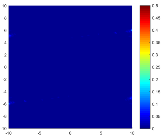
The size of the body is $10\times 10$ and the size of the disclination core is $0.5\times 0.5$ (in units of $t$, the core height). To compare our numerical solution with DeWit’s infinite-medium solutions, the following Neumann boundary conditions are utilized. Considering the body in our model as a patch in an infinite domain, the traction field on the boundary of the corresponding patch from the infinite-medium solution is applied. Figure 7(a) is the stress field $\sigma_{11}$ from the DeWit solution with Frank vector (30) and Figure 7(b) is the stress field $\sigma_{11}$ from small deformation g.disclination theory with the g.disclination density (31). Here, we denote $\mathbfit{\sigma}_{a}$ as the stress field from the analytical solution and $\mathbfit{\sigma}_{g}$ as the stress field from the g.disclination model. The difference between the analytical solution and the g.disclination solution is denoted as $\delta\sigma_{a,g}$ following the definition (1).

Figure 7(c) shows the defined difference of the stress field; the computed stress field from g.disclination theory matches with the DeWit solution very well. Outside the core, the defined difference is less than $1\%$.

We examine the difference between the stress fields from the small and finite deformation settings arising from a single disclination representing a high misorientation. For the small deformation problem, we assume the misorientation magnitude to be represented by $\tan\theta$, where $\theta$ is the misorientation, following (20). We set up a single disclination with a $45^{\circ}$ misorientation and apply traction-free boundary conditions. Figure 8(a) is the stress field from the small deformation setting and Figure 8(b) is that from the finite deformation setting. Figure 8(c) is the plot of the difference $\delta\sigma_{s,f}$, whose maximum is about $40\%$ and the mean of $\delta\sigma_{s,f}$ is $1.39\%$. It is clear that for large misorientations like the one shown (which is more than the commonly believed threshold of $>11^{\circ}$), there are significant differences between the small and finite deformation results.

Here we solve an edge dislocation problem, interpreted as a g.disclination dipole, as discussed in [ZA16, Sec. 4.3]. In this context, two opposite-sign g.disclinations are prescribed with the distortion differences as pure rotation differences (g.disclinations become pure disclinations), with Frank vector $\mathbfit{\Omega}$ and $-\mathbfit{\Omega}$ respectively. Based on the results in [ZA16], the Burgers vector ${\mathbfit b}$ for this disclination dipole in small deformation theory is given as ${\mathbfit b}=\mathbfit{\Omega}\times\delta{\mathbfit r}$, where $\delta{\mathbfit r}$ is the dipole vector (the vector that separates the two disclinations in the dipole).

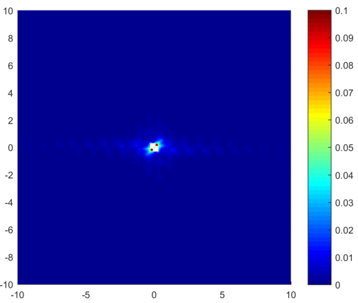
Figure 9(a) is the stress field $\sigma_{11}$ from the g.disclination dipole model and Figure 9(b) is the stress field $\sigma_{11}$ for the classical linear elastic dislocation with the corresponding Burgers vector ${\mathbfit b}=\mathbfit{\Omega}\times\delta{\mathbfit r}$. The traction boundary condition in the g.disclination dipole model is set to be that arising from the stress field of the corresponding classical linear elastic dislocation, following identical logic as in Section 5.3. $\mathbfit{\sigma}_{a}$ denotes the stress field of the classical linear elastic edge dislocation and $\mathbfit{\sigma}_{d}$ is the stress field from the g.disclination dipole model. The difference between the classical linear elasticity and the g.disclination dipole model is denoted as $\delta\sigma_{a,d}$ following definition (1). Figure 9(c) shows $\delta\sigma_{a,d}$. Outside the core, the stress fields from the g.disclination model match the one from the classical linear elastic dislocation very well.

As discussed in [ZA16], a grain boundary can be interpreted as a series of disclination dipoles. The elastic field of such a high-angle grain boundary is computed in this section. Also computed are the fields of a tilt grain boundary with disclination dipoles as well as with additional dislocations.

A disconnection is the region that connects two parallel grain boundary segments, referred to as terraces, that do not belong to a common plane. Extensive work on grain boundary disconnections have been done by Hirth, Pond and co-workers [HPH+13, HPL06]. They described the entire grain boundary as a series of terraces joined by disconnections. Figure 15 from [HPH+13] shows the terrace model and Figure 16 shows a schematic for understanding the reason for the occurrence of a disconnection. The terraces are assumed to contain misfit dislocations, and the disconnections are interpreted as additional dislocations located at the steps joining the terraces.

In this work, a disclination dipole model is introduced and computed to describe the grain boundary disconnection discussed in [HPH+13] shown in Figure 16. Figure 17 shows the thought experiment for representing the disconnection by a disclination dipole and a dislocation. According to g.disclination theory, we start from the current configuration of a disconnection that is represented by a disclination dipole and a dislocation, as shown in Figure 17(a). The red part is one grain and the blue part is another grain. The black dot at $A$ represents a negative disclination and the yellow dot at $B$ represents a positive disclination. Both disclinations have the same Frank vector magnitude $\Omega$ with opposite signs. The disclination density for each disclination is assumed to be derived from the difference of two (inverse) rotation matrices. The dislocation is located at $B$. The green lines represents the interface of the grain boundary. To get the reference configuration (the stress-free configuration shown in Figure 16(a), we need to relax the body by the following steps:

• •

  Cut the interface from the right end to $B$ and relax the negative disclination at $B$. Thus, the red part rotates clockwise by $\Omega$, generating an overlap wedge. The configuration after this step is shown in Figure 17(b).

• •

  Cut the interface from the $B$ to $A$ and relax the positive disclination at $A$. The red crystal rotates anticlockwise by $\Omega$. Therefore, the point $B$ on the red crystal moves to $C$ and there is now a gap wedge $CAB$. Furthermore, the overlap wedge generated by relaxing the negative disclination is counteracted by the opposite rotation in this step, as shown in Figure 17(c).

• •

  We now assume that the (true, F-S) Burgers vector of the dislocation at $B$ in Fig. 17(a) measured on the relaxed configuration is given by the vector joining $C$ to $D$ in Fig. 17(d). We now relax this dislocation.

Figure 18 shows the composite Burgers vector obtained from the above relaxation as a superposition of the Burgers vectors of the disclination dipole and the dislocation. It turns out that the Burgers vector from our model matches with the Burgers vector from [HPH+13]. Figure 18(a) is the Burgers vector diagram based on g.disclination theory - disclination densities are based on the inverse rotation matrices. Considering finite deformations, ${\mathbfit t}$ is rotated to ${\mathbfit s}$ by relaxing the disclinations and ${\mathbfit b}_{dipole}^{f}$ is denoted as the Burgers vector of the disclination dipole. Denote the i-elastic 1-distortion difference of the positive disclination as $\mathbfit{\Delta}$. The dipole separation vector in Figure 18(a) is ${\mathbfit t}$. Based on a result in [ZA16, Eqn(33)], the Burgers vector of the g.disclination dipole ${\mathbfit b}_{dipole}^{f}$ is given as

$${\mathbfit b}_{dipole}^{f}=\mathbfit{\Delta}{\mathbfit t}.$$

Assuming a completely in-plane problem, denote the rotation tensor acting on ${\mathbfit t}$ to produce ${\mathbfit s}$ in Figure 18(a) as ${\mathbfit R}$. The vector ${\mathbfit t}$ on the blue crystal is assumed to remain unchanged under the whole relaxation. Thus the i-elastic, 1-distortion difference is given by

$$\mathbfit{\Delta}={\mathbfit R}-{\mathbfit I},$$

with the matrix of ${\mathbfit R}$ (in any orthonormal basis) given by

$$\begin{bmatrix}\cos\Omega&&-\sin\Omega\\ \sin\Omega&&\cos\Omega\end{bmatrix}.$$

With reference to Fig. 18(a), ${\mathbfit b}_{dipole}^{f}$ can be written as

$${\mathbfit b}_{dipole}^{f}=({\mathbfit R}-{\mathbfit I}){\mathbfit t}={\mathbfit R}{\mathbfit t}-{\mathbfit t}={\mathbfit s}-{\mathbfit t}={\mathbfit u}$$

From the description shown in Figure 17, the Burgers vector of the dislocation, ${\mathbfit b}_{dislocation}^{f}$, can be written as ${\mathbfit b}_{dislocation}^{f}={\mathbfit v}-{\mathbfit s}={\mathbfit p}$. Therefore, the total Burgers vector of the disconnection is given by

$${\mathbfit b}_{total}^{f}={\mathbfit b}_{dipole}^{f}+{\mathbfit b}_{dislocation}^{f}={\mathbfit u}+{\mathbfit p}={\mathbfit q},$$

matching the result from [HPH+13]. Figure 18(b) is the Burgers vector diagram for the small deformation case. In this approximation, the dipole Burgers vector, ${\mathbfit b}_{dipole}^{s}$, is given by [ZA16, Eqn(7)]

$${\mathbfit b}_{dipole}^{s}=\mathbfit{\Omega}\times{\mathbfit t},$$

where $\mathbfit{\Omega}$ is the Frank vector of the positive disclination and is given by $tan\Omega{\mathbfit e}_{3}$ by (20). Then, ${\mathbfit b}_{dipole}^{s}$ can be written as

$${\mathbfit b}_{dipole}^{s}={\mathbfit u}^{\prime},$$

where ${\mathbfit u}^{\prime}$ is a vector perpendicular to ${\mathbfit t}$ with length $tan\Omega|t|$. The ‘rotated’ image of ${\mathbfit t}$ is ${\mathbfit s}^{\prime}={\mathbfit t}+{\mathbfit u}^{\prime}$. The Burgers vector of the dislocation ${\mathbfit b}_{dislocation}^{s}$ is ,

$${\mathbfit b}_{dislocation}^{s}={\mathbfit v}-{\mathbfit s}^{\prime}={\mathbfit p}^{\prime}$$

Thus, the total Burgers vector ${\mathbfit b}_{total}^{s}$ is given as

$${\mathbfit b}_{total}^{s}={\mathbfit b}_{dipole}^{s}+{\mathbfit b}_{dislocation}^{s}={\mathbfit u}^{\prime}+{\mathbfit p}^{\prime}.$$

References

- [AF12] Amit Acharya and Claude Fressengeas, Coupled phase transformations and plasticity as a field theory of deformation incompatibility, International journal of fracture 174 (2012), no. 1, 87–94.
- [AF15] , Continuum mechanics of the interaction of phase boundaries and dislocations in solids, Differential Geometry and Continuum Mechanics, Springer Proceedings in Mathematics and Statistics; Ed: G. Q. Chen, M. Grinfeld, R. J. Knops 137 (2015), 125–168.
- [AMK17] Hillel Aharoni, Thomas Machon, and Randall Kamien, Composite dislocations in smectic liquid crystals, Physical review letters 118 (2017), no. 25, 257801.
- [AR06] Amit Acharya and Anish Roy, Size effects and idealized dislocation microstructure at small scales: predictions of a phenomenological model of mesoscopic field dislocation mechanics: Part I, Journal of the Mechanics and Physics of Solids 54 (2006), no. 8, 1687–1710.
- [BAC05] Robert W. Balluffi, Sam Allen, and W. Craig Carter, Kinetics of materials, John Wiley & Sons, 2005.
- [Bha03] Kaushik Bhattacharya, Microstructure of martensite: why it forms and how it gives rise to the shape-memory effect, vol. 2, Oxford University Press, 2003.
- [BZB+12] Thomas R. Bieler, Bite Zhou, Lauren Blair, Amir Zamiri, Payam Darbandi, Farhang Pourboghrat, Tae-Kyu Lee, and Kuo-Chuan Liu, The role of elastic and plastic anisotropy of sn in recrystallization and damage evolution during thermal cycling in sac305 solder joints, Journal of Electronic Materials 41 (2012), no. 2, 283–301.
- [DeW72] R. DeWit, Partial disclinations, Journal of Physics C: Solid State Physics 5 (1972), no. 5, 529.
- [DeW73a] , Theory of disclinations. II- continuous and discrete disclinations in anisotropic elasticity, Journal of Research 77 (1973), 49–100.
- [DeW73b] , Theory of disclinations: Iv. straight disclinations, J. Res. Natl Bureau Standards Sect. A, Phys. Chem. A 77 (1973), 607–658.
- [Esh56] J. D. Eshelby, The continuum theory of lattice defects, Solid state physics 3 (1956), 79–144.
- [Esh57] John D. Eshelby, The determination of the elastic field of an ellipsoidal inclusion, and related problems, Proceedings of the Royal Society of London A: Mathematical, Physical and Engineering Sciences, vol. 241, The Royal Society, 1957, pp. 376–396.
- [GSJ+05] Y. Gao, L. Song, P. Jiang, L. F. Liu, X. Q. Yan, Z. P. Zhou, D. F. Liu, J. X. Wang, H. J. Yuan, Z. X. Zhang, et al., Silver nanowires with five-fold symmetric cross-section, Journal of crystal growth 276 (2005), no. 3, 606–612.
- [HLL+12] Christopher M. Hefferan, Jonathan Lind, Shiu Fai Li, Ulrich Lienert, Anthony D. Rollett, and Robert M. Suter, Observation of recovery and recrystallization in high-purity aluminum measured with forward modeling analysis of high-energy diffraction microscopy, Acta Materialia 60 (2012), no. 10, 4311–4318.
- [HPH+13] J. P. Hirth, R. C. Pond, R. G. Hoagland, X.-Y. Liu, and J. Wang, Interface defects, reference spaces and the Frank–Bilby equation, Progress in Materials Science 58 (2013), no. 5, 749–823.
- [HPL06] J. P. Hirth, R. C. Pond, and J. Lothe, Disconnections in tilt walls, Acta Materialia 54 (2006), no. 16, 4237–4245.
- [Jia98] B. Jiang, The least-squares finite element method, Springer, Berlin, 1998.
- [KNT+11] Stefan Kaufmann, Robert Niemann, Thomas Thersleff, Ulrich K. Rößler, Oleg Heczko, Jörg Buschbeck, Bernhard Holzapfel, Ludwig Schultz, and Sebastian Fähler, Modulated martensite: why it forms and why it deforms easily, New Journal of Physics 13 (2011), no. 5, 053029.
- [LIO98] V. I. Levitas, A. V. Idesman, and G. B. Olson, Continuum modeling of strain-induced martensitic transformation at shear-band intersections, Acta materialia 47 (1998), no. 1, 219–233.
- [Mer79] N. David Mermin, The topological theory of defects in ordered media, Reviews of Modern Physics 51 (1979), no. 3, 591.
- [Nab67] F. R. N. Nabarro, Theory of Crystal Dislocations (Monographs on Physics), Oxford University Press, 1967.
- [Nab85] , The development of the idea of a crystal dislocation, University of Tokyo Press, Tokyo, 1985.
- [Pur09] Saurabh Puri, Modeling dislocation sources and plastic flow through grain boundaries in mesoscopic field dislocation mechanics, Ph.D. thesis, Civil and Environmental Engineering, Carnegie Mellon University, 2009.
- [QYC+15] Qingquan Qin, Sheng Yin, Guangming Cheng, Xiaoyan Li, Tzu-Hsuan Chang, Gunther Richter, Yong Zhu, and Huajian Gao, Recoverable plasticity in penta-twinned metallic nanowires governed by dislocation nucleation and retraction, Nature communications 6 (2015).
- [RA05] Anish Roy and Amit Acharya, Finite element approximation of field dislocation mechanics, Journal of the Mechanics and Physics of Solids 53 (2005), no. 1, 143–170.
- [SGL11] Hanuš Seiner, Ondřej Glatz, and Michal Landa, A finite element analysis of the morphology of the twinned-to-detwinned interface observed in microstructure of the Cu–Al–Ni shape memory alloy, International Journal of Solids and Structures 48 (2011), no. 13, 2005 – 2014.
- [Shi73] R. T. Shield, The rotation associated with large strains, SIAM Journal on Applied Mathematics 25 (1973), no. 3, 483–491.
- [SW+71] Gene Simmons, Herbert Wang, et al., Single crystal elastic constants and calculated aggregate properties.
- [WBH12] J. Wang, I. J. Beyerlein, and J. P. Hirth, Nucleation of elementary and twinning dislocations at a twin boundary in hexagonal close-packed crystals, Modelling and Simulation in Materials Science and Engineering 20 (2012), no. 2, 024001.
- [ZA16] Chiqun Zhang and Amit Acharya, On the relevance of generalized disclinations in defect mechanics.