Subperiods and apparent pairing in integer quantum Hall interferometers
Abstract
We analyze the magnetic field and gate voltage dependence of the longitudinal resistance in an integer quantum Hall Fabry-Pérot interferometer, taking into account the interactions between an interfering edge mode, a non-interfering edge mode and the bulk. For weak bulk-edge coupling and sufficiently strong inter-edge interaction, we obtain that the interferometer operates in the Aharonov-Bohm regime with a flux periodicity halved with respect to the usual expectation. Even in the regime of strong bulk-edge coupling, this behavior can be observed as a subperiodicity of the interference signal in the Coulomb dominated regime. We do not find evidence for a connection between a reduced flux period and electron pairing, though. Our results can reproduce some recent experimental findings.
pacs
73.43.Cd, 85.35.Ds,73.23.HkPhase coherence is a key ingredient of quantum mechanics, and its consequences can be observed in interference experiments. We consider here the electronic version of a Fabry-Pérot interferometer (FPI) realized in the integer quantum Hall (QH) regime [1, 2, 3, 4, 5, 6, 7, 8, 9, 10], consisting of a Hall bar perturbed by two constrictions, which introduce amplitudes for backscattering. The probability that a particle is backscattered is determined by the interference of trajectories with a phase difference given by the Aharonov-Bohm flux enclosed by the loop. Due to the flux-sensitivity of the phase difference, the backscattering probability oscillates as a function of the magnetic field and a gate voltage used to change the interferometer area . There has been a renewed interest in QH interferometers because they allow to reveal anyonic statistics [11, 12, 13, 14, 15, 16, 17, 18, 19, 20, 21] with possible applications to quantum computation [22, 23].
Generally, QH interferometers come in two variants: Aharonov-Bohm (AB) and Coulomb dominated (CD) ones [5, 6, 4, 7, 24, 25, 2, 3, 8, 9, 10, 26, 27, 28]. The AB regime is characterized by a magnetic field periodicity and a gate voltage periodicity [2, 5], where denotes the flux quantum,
and . Moreover, the lines of constant interference phase in the two dimensional plane - have negative slope [6, 5], because the interference phase increases with both magnetic field and interferometer area,
and the latter grows when the gate voltage becomes more positive. One expects the AB signatures to be observed in large interferometers, when electrostatic interactions are weak. On the contrary, in small interferometers bulk and edge are strongly coupled, placing the interferometer in the CD regime. In this case, the lines of constant phase have positive slope in the - plane [10, 6, 5, 8], and a reduced magnetic field period is observed [3, 7, 6, 5], with denoting the filling fraction in the constriction region.
Recently, halving of the magnetic field and gate voltage period was observed experimentally [9] for a FPI with bulk filling factor between and , i.e., and . Interestingly, the observed negative slope of lines with constant phase is consistent with AB physics, while the reduced magnetic field period is reminiscent of CD physics. In addition,
shot noise measurements yield a Fano factor of two, indicating that the halving of the flux period could be interpreted in terms of electron pairing [9]. These intriguing experimental results are not explained by theoretical studies of Fabry-Pérot interferometers so far [24, 25, 26, 27, 29, 28].
In this Letter, we analyze a model which takes into account the electrostatic coupling of two modes as well as bulk-edge coupling, appropriate for modeling the experiment Ref. 9. We find that for
strong inter-edge coupling and weak bulk-edge interactions, the FPI is characterized by a negative slope of constant phase lines, together with halved magnetic field and gate voltage periodicity, in agreement with the experimental results [9]. We name this regime AB′. When adding one flux quantum, one electron is added to each edge mode, and due to the strong inter-edge coupling, this addition occurs in an alternating fashion between outer and inner edge. When an electron is added to the inner edge, it induces a phase shift on the outer edge such that
the oscillation period of the resistance is half a flux quantum. However, the analysis of the two-particle addition spectrum indicates that electron pairing is unlikely to occur for a wide range of parameters. We predict that an AB′ subleading contribution is still present even when the system is in the CD regime. Finally, we find that the transmission phase of a FPI embedded into a Mach-Zender interferometer (MZI) is described by AB physics, even for strong inter-edge coupling which places the FPI in the AB′ regime with regards to oscillations in the backscattering probability.
Model — We consider an electronic FPI at filling factor () in the limit of weak backscattering, as depicted in Fig. 1.
The outermost interfering edge encloses an area , giving rise to an interference phase . We decompose the area , where varies slowly with gate voltage, while represents a fluctuating part which is periodic in both magnetic field and gate voltage [25]. The charges in the inner edge mode and in the bulk are quantized, and are described by discrete variables .
Assuming that the area enclosed by the two edges and the bulk region are approximately equal, the charge imbalance in units of the electron charge is on the interfering edge, on the non-interfering edge, and in the bulk, with denoting the positive background charge, and with phase offsets and . Accordingly, the fluctuating part of the energy is given by
| (1) | |||
where the diagonal terms in represent the charging energies of the edges and the bulk, respectively. The off-diagonal terms encode the edge-edge coupling and the bulk-edge interaction . Considering all possible winding numbers of the electron around the interference cell, the longitudinal resistance due to backscattering is given by
| (2) |
where represents a thermal average at inverse temperature over the fluctuations with respect to the energy function given in Eq. (1). Here, , (, ) denote reflection and transmission amplitudes at QPC for particles travelling along the upper (lower) edge.
Phase diagram — We define the dimensionless parameters , and . We let to simplify the discussion. These values are generic in the sense that the results will not change qualitatively when using different parameters. For this choice, the system is energetically stable if and are satisfied. The expectation value of the interference phase in Eq. (2) is evaluated by first minimizing the quadratic energy Eq. (1) with respect to . To compute the remaining double sum over and we use the Poisson summation formula, and obtain
| (3) |
with , , and the definitions
| (4) | ||||
| (5) |
To leading order the denominator of Eq. (3) is unity, corresponding to . We now define , and use the expansion
| (6) |
Introducing , and considering the numerator for , we find
| (7) |
where the weight factors depend on the parameters , and also include the phase offsets. In Fig. 2 we indicate the regions in parameter space for which a given term in Eq. (7) is dominant.
These regions are characterized by the slope of lines with constant interference phase, the magnetic field period and the gate voltage period of the leading term of .
Interestingly, for strong edge-edge coupling and weak bulk-edge interactions the FPI is in the AB′ regime (see Fig. 2), characterized by a negative slope of constant phase lines,
together with halved flux and gate voltage periodicity.
Subleading corrections in the CD regime— Motivated by the experimental observation of a subleading AB component in a CD interferometer [10], we discuss the presence of a subleading AB′ component for a CD interferometer with larger filling in the following. To be specific, we consider and , placing the interferometer in the CD regime as in [10]. Accordingly, we find from Eq. (3)
| (8) |
with the complex numerical coefficients satisfying for . We now consider higher winding numbers
| (9) | ||||
| (10) |
with the complex numerical coefficients and .
Contributions with even higher windings are suppressed by powers and are thus less relevant.
We see from Eq. (8) that the leading term of the interference phase is independent of magnetic field,
and it has a gate voltage period .
Thus, the CD behavior dominates here and the lines of constant phase in the - plane are mainly straight, as shown in the inset of Fig. 3. Nevertheless,
also the AB′ component and higher harmonics are revealed in the oscillations of .
We note from Eq. (8) that for fixed the subleading frequencies are shifted by with respect to the dominant frequency. Moreover,
multiple windings in Eqs. (9), (10) translate a given frequency in Eq. (8) by integer multiples of . In order to formalize this observation, we introduce the 2D Fourier transform of as
| (11) |
Thus, a specific interference pattern corresponds to a set of points in Fourier space described by vectors , with and different from zero, , and the basis vectors defined as
| (12) |

In Fig. 3 we show a density plot of for , , and compare its peaks to the vectors in Eq. (12). We note that if also an additional subleading AB component would appear in the frequency spectrum of .
Addition and subtraction energies —
The general idea of Coulomb mediated pairing is that two electrons are added to one subsystem, while expelling one electron from another subsystem, which may be energetically favorable if
the interaction within a given subsystem is weaker than the interaction between different subsystems [30].
To explore this possibility, we now study a closed interferometer,
which displays the same magnetic field and gate voltage periods as obtained by analyzing the open limit of the FPI
[31].
Conductance maxima are now related to degeneracies of the energy with respect to changing the number
of electrons on the outer edge,
since tunneling is assumed to occur only into the outermost edge (scenario A).
Specifically, we compare the energy cost for adding, or subtracting, a single electron in the outermost edge with the corresponding energies for an electron pair in order to understand the transport processes occurring in the FPI.
We obtain an energy function from the one in Eq. (1) by setting , and then define the addition and subtraction energies , , allowing the number of electrons on the inner edge to relax in order to induce pairing. We plot both single particle and pair energies as a function of for weak and strong (AB′ phase).
As can be seen from Fig. 4, adding or subtracting a pair of electrons needs more energy than in the case of a single electron. Therefore, we argue that
tunneling of electron pairs is generally not favored by energetic considerations, although there are special paramter values
for which pair tunneling may be relevant [31].
In principle, there is the possibility that correlated sequential tunneling may be important, but a rate equation analysis needed to answer this question is beyond the scope of the present manuscript.
We next consider a scenario B, in which both inner and outer edge mode are contacted [32] and we allow the bulk to relax due to the presence of the Ohmic contact in the center of the interferometer [9]. We define the relaxed pair addition/subtraction energy . It is evident from Fig. 4 that electron pair tunneling can now occur for some values of flux when . Here, “pairing” refers to a process in which the tunneling of one electron to the outer edge and a second one to the inner edge happens either simultaneously or strongly correlated in time.
However, this scenario is not likely to be relevant for the experiment [9].
Transmission phase — We now consider a FPI placed in one of the two arms of a MZI [33], which allows to measure the transmission phase through the FPI (see inset of Fig. 5). If the FPI is symmetric, then the Coulomb contribution to the phase is shared equally between upper and lower edge, and we can express the MZI transmission probability as
| (13) |
where () are the transmission (reflection) amplitudes at the constrictions of the MZI and . The subtraction of is done in order to avoid double counting the FPI contribution to the MZI interference phase. Setting in Eq. (3), we obtain that
| (14) |
with and the weight factors depending on the values of and . We indicate in Fig. 5 the regions for which a given term in Eq. (14) dominates.
One sees that the phase diagram is almost completely composed of AB phase, where the FPI gate voltage and magnetic field periods are trivially doubled with respect to the AB periods of the longitudinal resistance due to the choice of (see Fig. 2). This behavior is independent of the edge-edge interaction strength . Only for large , a small region with CD features emerges. From Eqs. (13)-(14) we see that has the leading periodicity , and a subleading component with , even when such that interfering electrons do not encircle the interferometer cell. These findings are in agreement with the recent experiment [33].
Comparison with experiments — In the experiment [9] the FPI was found to be in the AB regime with magnetic field periodicity and gate voltage periodicity . At (representative of ) however, the periodicities are and , with the lines of constant phase still having negative slope. The AB phase at is theoretically described by the limit , and according to Fig. 2 we find and . Assuming that at the FPI is in the AB′ phase, the periodicities are and . Therefore, the experimentally
observed periodicities Ref. 9 are reproduced by our model. A discussion of current noise [9] and interference with multiple areas [33] are beyond the scope of the present manuscript.
Experimentally,
fingerprints of the AB phase in a CD-interferometer were reported in Ref. 10, and fingerprints of
the AB′ phase were observed at weaker magnetic field [34].
In particular, the dominant CD component had a gate voltage periodicity , and the subleading AB period was at () . According to our model, and at [31], yielding parameters and . Since depends linearly on the applied magnetic field and is independent of it,
for a weaker magnetic field (), we
expect a leading CD gate voltage period and a subleading AB′ period . These results are in agreement with recent experimental findings [34].
Conclusion — We propose a theoretical model for a FPI in which the outermost interfering edge interacts with the second non-interfering edge as well as with the bulk of the system. We find that for weak bulk-edge and strong edge-edge coupling the resistance oscillations are of AB type with halved flux periodicity (AB′ regime), in agreement with recent experimental results [9]. However, we do not find evidence for the importance of electron pair tunneling. We argue that there are fingerprints of AB′ physics even if the system is in the CD regime thanks to a partial screening of the bulk-edge interactions. We also calculate the transmission phase for a FPI situated in one arm of a MZI.
Acknowledgements — We would like to thank M. Heiblum and I. Sivan for helpful discussions and for sharing unpublished results, and the German Science Foundation (DFG) for financial support via grant RO 2247/8-1.
References
- [1] C. de C. Chamon, D. E. Freed, S. A. Kivelson, S. L. Sondhi, and X. G. Wen, Phys. Rev. B 55, 2331 (1997).
- [2] F. E. Camino, W. Zhou, and V. J. Goldman, Phys. Rev. B 72, 155313 (2005).
- [3] F. E. Camino, W. Zhou, and V. J. Goldman, Phys. Rev. B 76, 155305 (2007).
- [4] D. T. McClure, Y. Zhang, B. Rosenow, E. M. Levenson-Falk, C. M. Marcus, L. N. Pfeiffer, and K. W. West, Phys. Rev. Lett. 103, 206806 (2009).
- [5] Y. Zhang, D. T. McClure, E. M. Levenson-Falk, C. M. Marcus, L. N. Pfeiffer, and K. W. West, Phys. Rev. B 79, 241304 (2009).
- [6] N. Ofek, A. Bid, M. Heiblum, A. Stern, V. Umansky, and D. Mahalu, Proceedings of the National Academy of Sciences 107, 5276 (2010).
- [7] H. Choi, P.-h. Jiang, M. Godfrey, W. Kang, S. Simon, L. Pfeiffer, K. West, and K. Baldwin, New Journal of Physics 13, 055007 (2011).
- [8] D. T. McClure, W. Chang, C. M. Marcus, L. N. Pfeiffer, and K. W. West, Phys. Rev. Lett. 108, 256804 (2012).
- [9] H. Choi, I. Sivan, A. Rosenblatt, M. Heiblum, V. Umansky, and D. Mahalu, Nature communications 6 (2015).
- [10] I. Sivan, H. Choi, A. Rosenblatt, J. Park, Y. Gefen, D. Mahalu, and V. Umansky, Nature communications 7 (2016).
- [11] J. M. Leinaas and J. Myrheim, Il Nuovo Cimento B (1971-1996) 37, 1 (1977).
- [12] F. Wilczek, Phys. Rev. Lett. 48, 1144 (1982a).
- [13] F. Wilczek, Phys. Rev. Lett. 49, 957 (1982b).
- [14] D. Arovas, J. R. Schrieffer, and F. Wilczek, Phys. Rev. Lett. 53, 722 (1984).
- [15] A. Stern, Nature 464, 187 (2010).
- [16] A. Stern and B. I. Halperin, Phys. Rev. Lett. 96, 016802 (2006).
- [17] P. Bonderson, A. Kitaev, and K. Shtengel, Phys. Rev. Lett. 96, 016803 (2006).
- [18] R. L. Willett, L. N. Pfeiffer, and K. W. West, Proceedings of the National Academy of Sciences 106, 8853 (2009).
- [19] R. L. Willett, L. N. Pfeiffer, and K. W. West, Phys. Rev. B 82, 205301 (2010).
- [20] R. L. Willett, C. Nayak, K. Shtengel, L. N. Pfeiffer, and K. W. West, Phys. Rev. Lett. 111, 186401 (2013).
- [21] C. W. von Keyserlingk, S. H. Simon, and B. Rosenow, Phys. Rev. Lett. 115, 126807 (2015).
- [22] C. Nayak, S. H. Simon, A. Stern, M. Freedman, and S. Das Sarma, Rev. Mod. Phys. 80, 1083 (2008).
- [23] S. Das Sarma, M. Freedman, and C. Nayak, Phys. Rev. Lett. 94, 166802 (2005).
- [24] B. Rosenow and B. I. Halperin, Phys. Rev. Lett. 98, 106801 (2007).
- [25] B. I. Halperin, A. Stern, I. Neder, and B. Rosenow, Phys. Rev. B 83, 155440 (2011).
- [26] S. Ngo Dinh and D. A. Bagrets, Phys. Rev. B 85, 073403 (2012).
- [27] S. N. Dinh, D. A. Bagrets, and A. D. Mirlin, Annals of Physics 327, 2794 (2012).
- [28] S. Baer and K. Ensslin, Transport spectroscopy of confined fractional quantum Hall systems, Vol. 183 (Springer, 2015).
- [29] D. Ferraro and E. Sukhorukov, ArXiv e-prints (2016), arXiv:1608.08889 .
- [30] A. Hamo, A. Benyamini, I. Shapir, I. Khivrich, J. Waissman, K. Kaasbjerg, Y. Oreg, F. von Oppen, and S. Ilani, Nature 535 (2016).
- [31] See supplementary material .
- [32] S. Baer, C. Rössler, T. Ihn, K. Ensslin, C. Reichl, and W. Wegscheider, New Journal of Physics 15, 023035 (2013).
- [33] I. Sivan, R. Bhattacharyya, H. Choi, M. Heiblum, D. Feldman, D. Mahalu, and V. Umansky, arXiv:1707.06818 (2017).
- [34] Private communication .
Supplementary material for "Subperiods and apparent pairing in integer quantum Hall interferometers"
I S1. Calculation of the interference phase
We provide here some details about the calculation of the interference phase . We define the dimensionless parameters , , where in the inverse temperature . In the open limit, we can evaluate the thermal expectation value
| (S1) |
where the partition function is
| (S2) |
We note that the energy defined in the main text is quadratic in the variable , hence to obtain Eq. (S1) and Eq. (S2) we just solved a Gaussian integral. The summations over the discrete degrees of freedom , can be managed through the Poisson summation formula
| (S3) |
Hence, Eq. (S3) allows to integrate over instead of summing, and we obtain that
| (S4) |
with and the function defined as
| (S5) |
If we assume equal charging energies for the bulk and the edges, i.e., , Eq. (S5) coincide with Eq. (5) in the main text. First of all, we consider the leading order of the Eq. (S4). We focus only on the numerator because to leading order the denominator is equal to unity, since its dominant term given by the duple . The integers and that give rise to the dominant term in the numerator depend on the value of and . We note that varying and does not affect the phase diagram in a qualitative way; moreover the phase diagram is independent of the parameters and . The AB′ phase is extended by increasing , while the CD phases expand with an increase of . The interesting AB′ phase always appears in the phase diagram if .
II S2. Subleading corrections to the interference phase
In the following we set and consider the limit of strong edge-edge coupling, i.e. . Therefore, Eq. (S4) simplifies to
| (S6) |
with the function defined as
| (S7) |
because we need to keep only the term in the numerator of Eq. (S4) and in the denominator . The leading term of the denominator in Eq. (S6) is given by , while its -th sub-leading term is a result of the terms. From these considerations and from the Taylor expansion of , we obtain that
| (S8) |
We note that this result is valid for any value of the edge-bulk coupling . For the leading behavior and subleading corrections of the numerator in Eq. (S6) are
| (S9) | ||||
| (S10) | ||||
| (S11) |
Considering small variation of gate voltage and magnetic field from an initial value , we have and . Defining and combining Eq. (S8) with Eqs. (S9)-(S10)-(S11), we obtain the Eqs. (8)-(9)-(10) in the main text.
III S3. Interferometer at )
In the case the FPI consists of a single interfering edge and the bulk, the energy function is
| (S12) |
Proceeding as before, we obtain in this case that
| (S13) |
with given by Eq. (S7). The dominant term in the denominator is ; on the other hand the leading term of the numerator depends on the value of [1]. The -th subleading term of the denominator is given by terms. Therefore, we obtain from the Taylor expansion that
| (S14) |
We now set ; our choice is motivated by the experimental setup in [2]. In this case we can write the numerator as
| (S15) | ||||
| (S16) |
Combining Eq. (S14) with Eqs. (S15)-(S16), the oscillatory part of the resistance in terms of and is
| (S17) | ||||
| (S18) |
where and , with .
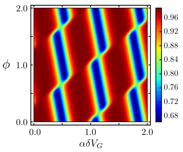

Therefore, thanks to a partial screening of the edge-bulk interaction, the resistance displays also AB component and higher harmonics other than the dominant CD term. From Eqs. (S17)-(S18), we can identify the peaks of the 2D Fourier transform of with vectors (see Fig.S1), with and different from zero, , and with the two reciprocal lattice vectors now defined as
| (S19) |
Fourier components show up in the experimental results [2], while these are missing in our theoretical analysis so far. The lack of the terms with is caused by our assumption that the backscattering amplitudes are independent of the charge in the bulk. If we assume a linear dependence of , we find that the additional frequency arise from the direct term .
IV S4. Pairing scenarios
We now consider the model in the closed limit, with representing the quantized charge in the interfering edge mode.
Despite its simplicity, our model in principle allows for electron pairing to occur, in case the mutual Coulomb repulsion energetically favors such processes with changes of in one of the edges. We have identified two distinct mechanisms that feature a sequence of transitions in the groundstate stability diagram of the closed system relevant for pairing. The first case corresponds to scenario A of the main text, and is realized for and in the vicinity of the unstable point of the quadratic form Eq.(1) in the main text. Without loss of generality, we neglect the bulk and set . The system first undergoes a flux-induced charge re-distribution as and as the flux is further increased, a transition followed by a redistribution , with the total charge increased only by . In Fig. S3 we show the stability diagram containing the relevant groundstate sequence. The repulsion needs to have a minimal strength, depending on the precise value of , to stabilize this groundstate sequence. As the coupling is further increased for , additional transitions with increasing appear in the stability diagram, until the system eventually becomes unstable.
If on the other hand, it is energetically more favourable to place a single additional charge into and to leave unchanged, instead of adding two charges to and redistributing charge afterwards. In the symmetric limit , , and hence the "pairing regime" lies in the unstable regime.
For the second pairing mechanism in scenario B, the Coulomb repulsion between edges and bulk is the relevant coupling. We assume and . As the flux is increased by one flux quantum, the number of bulk particles decreases by , typically in two separate groundstate transitions, while the edge charges increase by each. The role of is to ‘synchronize’ these transitions as a function of the flux, such that
. The synchronization is eventually destroyed for some finite value of
, where now the sequence of transitions takes place. The synchronization turns out to be stable for .
Scenario A
Scenario B
Scenario A

Scenario B
V S5. Conductance in the closed limit
The conductance in the closed limit can be calculated via the fluctuation-dissipation theorem, , where is the diffusion rate for motion of electrons inside or outside the interfering edge [3]
| (S20) |
with denoting the Fermi distribution, contains the tunneling matrix elements which we assume to be constant for simplicity and are the addiction/subtraction energies of one electron from the interfering edge mode. We present in Fig. S4 the density plot of the conductance as a function of and obtained from Eq. (S20) for different values of the couplings. We note that the slope of the lines of constant phase and the periodicities of the conductance coincide with the one calculated in the open limit. Therefore, the results achieved in the open limit are valid also for the closed limit. Moreover, the conductance is maxim/minimum when , evaluated in the ground state configuration, is minimum/maxim, as it can be seen from comparison of Fig. S4 with Fig. (4) in the main text. This is something expected, indeed the conductance is big/small when we need a small/big amount of energy for adding, or subtracting, an electron.


References
- [1] B. I. Halperin, A. Stern, I. Neder, and B. Rosenow, Phys. Rev. B 83, 155440 (2011).
- [2] I. Sivan, H. Choi, A. Rosenblatt, J. Park, Y. Gefen, D. Mahalu, and V. Umansky, Nature communications 7 (2016).
- [3] B. Rosenow and B. I. Halperin, Phys. Rev. Lett. 98, 106801 (2007).