跳到论文正文
W Papers独立论文阅读器 arXiv:1709.04390 论文正文 计算阅读时间 · 0%
引用这篇论文根据当前论文元数据生成,正式投稿前建议核对。


License: arXiv.org perpetual non-exclusive license
arXiv:1709.04390v2 [math.NA] 11 Jun 2018

FESTUNG: A MATLAB / GNU Octave toolbox for the discontinuous Galerkin method. Part III: Hybridized discontinuous Galerkin (HDG) formulation

Alexander Jaust Email: alexander.jaust@uhasselt.be Address: UHasselt – Hasselt University, Faculty of Sciences, Agoralaan Gebouw D, 3590 Diepenbeek, Belgium    Balthasar Reuter Email: reuter@math.fau.de Address: Friedrich–Alexander University of Erlangen–Nürnberg, Department of Mathematics, Cauerstraße 11, 91058 Erlangen, Germany    Vadym Aizinger Email: vadym.aizinger@awi.de Address: Friedrich–Alexander University of Erlangen–Nürnberg, Department of Mathematics, Cauerstraße 11, 91058 Erlangen, Germany Address: Alfred Wegener Institute, Helmholtz Centre for Polar and Marine Research, Am Handelshafen 12, 27570 Bremerhaven, Germany Corresponding author: Corresponding author    Jochen Schütz Email: jochen.schuetz@uhasselt.be Address: UHasselt – Hasselt University, Faculty of Sciences, Agoralaan Gebouw D, 3590 Diepenbeek, Belgium    Peter Knabner Email: knabner@math.fau.de Address: Friedrich–Alexander University of Erlangen–Nürnberg, Department of Mathematics, Cauerstraße 11, 91058 Erlangen, Germany
Abstract

The third paper in our series on open source MATLAB / GNU Octave implementation of the discontinuous Galerkin (DG) method(s) focuses on a hybridized formulation. The main aim of this ongoing work is to develop rapid prototyping techniques covering a range of standard DG methodologies and suitable for small to medium sized applications. Our FESTUNG package relies on fully vectorized matrix / vector operations throughout, and all details of the implementation are fully documented. Once again, great care is taken to maintain a direct mapping between discretization terms and code routines as well as to ensure full compatibility to GNU Octave. The current work formulates a hybridized DG scheme for a linear advection problem, describes hybrid approximation spaces on the mesh skeleton, and compares the performance of this discretization to the standard (element-based) DG method for different polynomial orders.

Keywords:
MATLAB, GNU Octave , hybridized discontinuous Galerkin (HDG) method, vectorization, open source , diagonally implicit Runge-Kutta method (DIRK)

1 Introduction

The discontinuous Galerkin (DG) method first introduced in the early 70s in [1] went on to have an illustrious career as one of the most popular numerical methods especially (but not exclusively) for fluid simulation and engendered a whole family of numerical schemes (see, e.g. [2, 3] and the references therein). The reasons for this success are many [4, 5]: an extremely flexible framework easily lending itself to many different types of equations, stability and conservation properties comparable to those of the finite volume method, natural support for high order discretizations and various types of adaptivity (hh-, pp-, rr-) as well as for complex domain geometries, etc. Due to a favorable computation-to-communication ratio, the method also fits extremely well into the popular parallel and hybrid computational paradigms [6].

However, one aspect of the DG methodology places it at a clear disadvantage compared to the classical finite element and finite volume methods: a large number of degrees of freedom with corresponding memory requirements. This drawback becomes even more restrictive in time-implicit or stationary numerical solvers that rely on matrix assembly, where increases in the lengths of vectors of unknowns become quadratically compounded in the sizes of corresponding matrix blocks. One idea proposed to speed up the solution of linear systems resulting from DG discretizations exploits the specifics of DG approximation spaces. Since DG basis functions are usually element-local (and often also hierarchical), the linear system can be trivially split into parts corresponding to different polynomial orders resulting in a scheme somewhat inspired by multigrid solvers, where different polynomial approximations on a fixed mesh play the role of fine and coarse mesh solutions of the classical multigrid. This approach can be carried out for each polynomial degree as in the pp-multigrid method [7, 8, 9] or using a two scale technique as in the hierarchical scale separation (HSS) method or variations thereof [10, 11, 12, 13]. Another common way to deal with this issue—and in many cases even to speed up the time-to-solution [14, 15, 16]—is to use hybridization. Roughly speaking, this means that the discretized PDE is augmented with an unknown—let us call it λh\lambda_{h}—supported on the skeleton of the mesh consisting of element edges in 2D and element faces in 3D. Using static condensation on the algebraic system level produces a significantly smaller system than that obtained for an unhybridized DG method at the price of additional cell-wise (small and uncoupled) linear systems that have to be solved alongside the globally coupled system on the mesh skeleton. Since all local solves are element-local and fully decoupled, the parallel communication cost of this algorithm part is zero.

The idea of using hybridization can be traced back to the 60s [17], it has subsequently been used in the context of mixed methods [18, 19]. In those works, λh\lambda_{h} was not only considered an implementation feature but also as a way to obtain a more accurate solution via postprocessing. Based on the work in [20], Cockburn and coworkers introduced the hybridized discontinuous Galerkin method in a unifying framework in [21]. Subsequently, the method has been extended to various types of equations such as the Stokes [22, 23] and Darcy-Stokes equations [24], the incompressible and compressible Navier-Stokes equations [25, 26, 27, 28], the Maxwell equations [29], and—particularly relevant for this work—the convection(-diffusion) equation [30, 31, 32]. For an interesting unification framework, we would also like to draw reader’s attention to a recent publication [33].

The current work applies and extends to the hybridized schemes the framework and design principles introduced in [34, 35] for unhybridized DG formulations and epitomized in our MATLAB / GNU Octave toolbox FESTUNG (Finite Element Simulation Toolbox for UNstructured Grids) available at [36, 37]. Citing from [34], we aim to

  1. 1.

    Design a general-purpose software package using the DG method for a range of standard applications and provide this toolbox as a research and learning tool in the open source format.

  2. 2.

    Supply a well-documented, intuitive user-interface to ease adoption by a wider community of application and engineering professionals.

  3. 3.

    Relying on the vectorization capabilities of MATLAB / GNU Octave, optimize the computational performance of the toolbox components and demonstrate these software development strategies.

  4. 4.

    Maintain throughout full compatibility with GNU Octave to support users of open source software.

For details about basic data structures and a general overview of the solver structure, we refer the interested reader to our first publication [34], which applies the local discontinuous Galerkin (LDG) method to the diffusion operator. A DG discretization of the same model problem as in this work combined with higher-order explicit time stepping schemes and arbitrary order vertex-based slope limiters [38, 39] is presented in the second paper in series [35]. The implementation presented in the current publication makes use of a new solver structure tailored towards improved readability and maintainability of the code and designed to ease coupling of different solvers. A detailed description of this new structure with an outline of the coupling capabilities is in preparation [40].

The rest of the paper is structured as follows: The model problem is introduced in the next section accompanied by a detailed description of the space and time discretization in Section 3. Important aspects of the implementation including local mappings, numerical quadrature, and the assembly of the system matrix are presented in Section 4. In Section 5, the code is verified using analytical convergence tests, and the numerical results are compared to those of the unhybridized DG implementation of the model problem from our previous publication [35]. Section 6 lists the routines mentioned in this article, and Section 7 contains some conclusions and a brief outlook of future tasks.

2 Model problem

Let J≔(0,tend)J\coloneqq(0,t_{\mathrm{end}}) be a finite time interval, and let Ω⊂ℝ2\Omega\subset\mathds{R}^{2} be a polygonally bounded Lipschitz domain with boundary ∂Ω\partial\Omega. We solve the linear advection equation

∂tc⁡(t,𝐱)+∇⋅𝐟⁡(t,𝐱,c⁡(t,𝐱))=ξ⁡(t,𝐱)in​J×Ω,\partial_{t}\,c\,(t,\mathbf{x})+\nabla\cdot\mathbf{f}\,\left(t,\mathbf{x},c\,(t,\mathbf{x})\right)=\xi\,(t,\mathbf{x})\quad\text{in}\;J\times\Omega\,, (1)

where the scalar quantity c:J×Ω→ℝc:J\times\Omega\rightarrow\mathds{R} is unknown. The flux function 𝐟:J×Ω×ℝ→ℝ2\mathbf{f}{}:J\times\Omega\times\mathds{R}\rightarrow\mathds{R}^{2} determines the type of the problem and may depend on time tt and space coordinate 𝐱\mathbf{x}. Within the context of this work, we assume

𝐟⁡(t,𝐱,c⁡(t,𝐱))≔[u1​(t,𝐱),u2​(t,𝐱)]T​c​(t,𝐱)\mathbf{f}\,\left(t,\mathbf{x},c\,(t,\mathbf{x})\right)\coloneqq{\begin{bmatrix}u^{1}(t,\mathbf{x}),&u^{2}(t,\mathbf{x})\end{bmatrix}}^{\mathrm{T}}\,c\,(t,\mathbf{x})\, (2)

with given velocity 𝐮≔[u1,u2]T\mathbf{u}\coloneqq{[u^{1},u^{2}]}^{\mathrm{T}} and source function ξ:J×Ω→ℝ\xi:J\times\Omega\rightarrow\mathds{R} independent of cc. Additionally, Eq. (1) is equipped with some initial

c=c0on​{0}×Ωc\;=\;c^{0}\quad\text{on}\penalty\ \{0\}\times\Omega (3)

and Dirichlet boundary condition

c=cDon​J×∂Ωin​(t)c\;=\;c_{\mathrm{D}}\quad\text{on}\penalty\ J\times{\partial\Omega}_{\mathrm{in}}(t) (4)

on inflow boundaries ∂Ωin​(t)≔{𝐱∈∂Ω|𝐮⁡(t,𝐱)⋅𝝂⁡(𝐱)<0}\partial\Omega_{\mathrm{in}}(t)\coloneqq\{\mathbf{x}\in\partial\Omega\,|\,\mathbf{u}(t,\mathbf{x})\cdot\boldsymbol{\nu}(\mathbf{x})<0\} with 𝝂⁡(𝐱)\boldsymbol{\nu}(\mathbf{x}) denoting the outward pointing unit normal vector. Since (1) specifies a first-order hyperbolic equation, no boundary conditions need to be prescribed on the outflow boundary ∂Ωout​(t)≔∂Ω∖Ωin​(t)\partial\Omega_{\mathrm{out}}(t)\coloneqq\partial\Omega\setminus\Omega_{\mathrm{in}}(t). Functions c0:Ω↦ℝc^{0}:\Omega\mapsto\mathds{R} and cD:J×∂Ωin​(t)↦ℝc_{\mathrm{D}}:J\times\partial\Omega_{\mathrm{in}}(t)\mapsto\mathds{R} are given. The model problem is the same as the one considered in the second paper of our series [35]; however, a slightly different notation is used here.

3 Discretization

3.1 Notation

Let 𝒯h={T}\mathcal{T}_{h}=\{T\} be a regular family of non-overlapping partitions of a polygonally bounded domain Ω\Omega into KK closed triangles TT. The hybridized discontinuous Galerkin scheme employed in this work uses unknowns located on element boundaries, i.e., on the edges of elements (also referred to as the trace of the mesh). We introduce the set of all edges ℰh=ℰint∪ℰext\mathcal{E}_{h}=\mathcal{E}_{\text{int}}\cup\mathcal{E}_{\text{ext}} consisting of sets of interior edges ℰint\mathcal{E}_{\text{int}} and boundary edges ℰext\mathcal{E}_{\text{ext}}. The latter is split into inflow ℰin\mathcal{E}_{\text{in}} and outflow edges ℰout\mathcal{E}_{\text{out}}. Furthermore, on each edge Ek¯∈ℰhE_{\bar{k}}\in\mathcal{E}_{h}, a unit normal 𝝂k¯\boldsymbol{\nu}_{\bar{k}} is defined such that 𝝂k¯\boldsymbol{\nu}_{\bar{k}} is exterior to element Tk¯−T_{\bar{k}^{-}}, where Tk¯−T_{\bar{k}^{-}} is an arbitrarily chosen but fixed element adjoining Ek¯E_{\bar{k}}. Obviously, boundary edges have only one adjacent element. For interior edges, the element opposite to Tk¯−T_{\bar{k}^{-}} is called Tk¯+T_{\bar{k}^{+}}. The minus sign in Tk¯−T_{\bar{k}^{-}} is suppressed when no confusion is possible. The total number of edges is denoted by

K¯≔|ℰh|,andΓ=⋃k¯=1K¯Ek¯\mkern 1.5mu\overline{\mkern-1.5muK\mkern-1.5mu}\mkern 1.5mu\coloneqq|\mathcal{E}_{h}|,\qquad\mbox{and}\qquad\Gamma=\bigcup_{\bar{k}=1}^{\mkern 1.5mu\overline{\mkern-1.5muK\mkern-1.5mu}\mkern 1.5mu}E_{\bar{k}}

is the trace of the mesh. We refer to elements using indices kk, and add bars ⋅¯\bar{\cdot} (e.g., k¯\bar{k} or K¯\mkern 1.5mu\overline{\mkern-1.5muK\mkern-1.5mu}\mkern 1.5mu) whenever we refer to edges to distinguish one from another. Additionally, we make use of the notation from the previous publications [34, 35] where we referred to edges of an element TkT_{k} as Ek​n,n∈{1,2,3}E_{kn},n\in\{1,2,3\}. Note the difference between this element-local edge numbering (“Ek​nE_{kn} is the nnth edge of the kkth element”) and global edge numbering (“Ek¯E_{\bar{k}} is the k¯\bar{k}th edge in the mesh”).

For the description of the method, we need mappings allowing us to switch back and forth between element-local and global indices. For that reason, we introduce a mapping ρ⁡(k,n)\rho(k,n) that relates the nnth edge Ek​nE_{kn} of element TkT_{k} to its global index in the set of edges ℰh\mathcal{E}_{h}

ρ:{1,…,K}×{1,2,3}→{1,…,K¯},(k,n)↦k¯.\rho:\{1,\ldots,K\}\times\{1,2,3\}{\rightarrow\{1,\ldots,\mkern 1.5mu\overline{\mkern-1.5muK\mkern-1.5mu}\mkern 1.5mu\},\quad}(k,n)\mapsto\bar{k}\,. (5)

This mapping is not injective since for each interior edge there exists a pair of index tuples (k−,n−)(k^{-},n^{-}) and (k+,n+)(k^{+},n^{+}) that map to the same edge index k¯\bar{k}, i. e., Ek¯=Ek−​n−=Ek+​n+E_{\bar{k}}=E_{k^{-}n^{-}}=E_{k^{+}n^{+}} (cf. Fig. 1). We define a second mapping κ⁡(k¯,l)\kappa(\bar{k},l) to identify elements Tk−,Tk+T_{k^{-}},T_{k^{+}} adjacent to an edge Ek¯E_{\bar{k}}. In this, argument l∈{1,2}l\in\{1,2\} denotes the edge-local index of the adjacent elements; it is constructed so that l=1l=1 refers to the “inner” element Tk−T_{k^{-}} (that always exists) while l=2l=2 refers to the “outer” element Tk¯+T_{\bar{k}^{+}} that exists only for interior edges ℰint\mathcal{E}_{\mathrm{int}},

κ:{1,…,K¯}×{1,2}→{0,…,K},(k¯,l)↦{k−∈{1,…,K},if ​l=1k+∈{0,…,K},if ​l=2}.\kappa:\{1,\ldots,\mkern 1.5mu\overline{\mkern-1.5muK\mkern-1.5mu}\mkern 1.5mu\}\times\{1,2\}{\rightarrow\{0,\ldots,K\},\quad}(\bar{k},l)\mapsto\left\{\begin{matrix}k^{-}\in\{1,\ldots,K\}\,,&\text{if }l=1\\ k^{+}\in\{0,\ldots,K\}\,,&\text{if }l=2\end{matrix}\right\}\,. (6)

As element indices start counting from 1, we set κ⁡(k¯,2)=0,∀Ek¯∈ℰext\kappa(\bar{k},2)=0\,,\forall E_{\bar{k}}\in\mathcal{E}_{\text{ext}} to mark the absence of the “outer” element.

Figure 1: Two triangles adjacent to edge Ek¯{E_{\bar{k}}}. It holds Ek¯=Ek−​n−=Ek+​n+{E_{\bar{k}}=}E_{k^{-}n^{-}}=E_{k^{+}n^{+}} and νk−​n−=−νk+​n+\mathbf{\nu}_{k^{-}n^{-}}=-\mathbf{\nu}_{k^{+}n^{+}}.

3.2 Semi-discrete form and hybridization

The particular feature of the HDG method that distinguishes it from conventional DG methods is that solutions are not only sought on elements, but also on the skeleton of the mesh. To this end, one has to define approximation spaces on both 𝒯h\mathcal{T}_{h} and ℰh\mathcal{E}_{h}. Given ℙp​(T)\mathds{P}_{p}(T) and ℙp​(E)\mathds{P}_{p}(E), the spaces of complete polynomials of degree at most pp on an element T∈𝒯hT\in\mathcal{T}_{h} and edge E∈ℰhE\in\mathcal{E}_{h}, respectively, we denote global broken polynomial spaces ℙp​(𝒯h),ℙp​(ℰh)\mathds{P}_{p}(\mathcal{T}_{h}),\mathds{P}_{p}(\mathcal{E}_{h}) on the triangulation 𝒯h\mathcal{T}_{h} and its set of edges ℰh\mathcal{E}_{h} by

ℙp(𝒯h)≔{φh:Ω¯→ℝ:∀T∈𝒯h,φh|T∈ℙp(T)},ℙp(ℰh)≔{μh:Γ→ℝ:∀E∈ℰh,μh|E∈ℙp(E)}.{\mathds{P}_{p}(\mathcal{T}_{h})}\coloneqq\{\varphi_{h}:\bar{\Omega}\rightarrow\mathbb{R}:\;\forall T\in\mathcal{T}_{h},\;\varphi_{h}|_{T}\in\mathbb{P}_{p}(T)\}\,,\qquad{\mathds{P}_{p}(\mathcal{E}_{h})}\coloneqq\{\mu_{h}:\Gamma\rightarrow\mathbb{R}:\;\forall E\in\mathcal{E}_{h},\;\mu_{h}|_{E}\in\mathbb{P}_{p}(E)\}\,. (7)

To support the tutorial character of this paper, we briefly discuss the derivation of the HDG method for the advection equation and refer the reader to [31] for more details. The standard DG discretization of (1) is obtained by multiplying (1) with a test function φh∈ℙp​(𝒯h)\varphi_{h}\in\mathds{P}_{p}(\mathcal{T}_{h}), applying integration by parts on element Tk∈𝒯h{T_{k}}\in\mathcal{T}_{h}, and replacing the flux 𝐟\mathbf{f} (see (2)) on element boundaries ∂Tk\partial{T_{k}} by a numerical flux function 𝐟^D​G​(ch−,ch+)\hat{\mathbf{f}}_{DG}(c^{-}_{h},c^{+}_{h}) well-known from finite volume discretizations [41, 42, 43] that depends on the values of the solution chc_{h} from both sides of the boundary of element Tk∈𝒯h{T_{k}}\in\mathcal{T}_{h}. Omitting the time argument of chc_{h} in the flux function for the sake of readability, this yields

∫Tk∂tch(t)φhd𝐱−∫Tk𝐟(ch)⋅∇φhd𝐱+∫∂Tk𝐟^D​G(ch−,ch+)⋅𝝂Tkφhds\displaystyle\int_{T_{k}}\partial_{t}c_{h}(t)\,\varphi_{h}\,\text{d}\mathbf{x}-\int_{T_{k}}\mathbf{f}\,\left(c_{h}\right)\cdot\nabla\varphi_{h}\,\text{d}\mathbf{x}+\int_{\partial{T_{k}}}\hat{\mathbf{f}}_{DG}(c^{-}_{h},c^{+}_{h})\cdot\boldsymbol{\nu}_{{T_{k}}}\,{\color[rgb]{1,0,0}{\varphi_{h}}}\,\text{d}s =∫Tkξ⁡(t)​φh​d​𝐱\displaystyle\,=\,\int_{T_{k}}\xi{{(t)}}\,\varphi_{h}\,\text{d}\mathbf{x}\,\quad ∀φh∈ℙp​(𝒯h).\displaystyle\forall\varphi_{h}\in\mathds{P}_{p}(\mathcal{T}_{h})\,. (8)

At the domain boundary ∂Ω\partial\Omega, ch+c^{+}_{h} has of course to be replaced by a suitably chosen boundary value c∂Ω​(ch−)c_{\partial\Omega}(c^{-}_{h}) as in

c∂Ω​(ch−)={ch−,on outflow boundary ∂Ωout,cD,on inflow boundary ∂Ωin.\displaystyle c_{\partial\Omega}(c^{-}_{h})=\begin{cases}c^{-}_{h},\quad\text{on outflow boundary ${\partial\Omega}_{\mathrm{out}}$}\,,\\ c_{D},\quad\text{on inflow boundary ${\partial\Omega}_{\mathrm{in}}$}\,.\end{cases} (9)

In this work, the numerical flux is chosen to be a slightly modified local Lax-Friedrichs/Rusanov flux [44, 45]

𝐟^D​G​(ch−,ch+)≔𝐟⁡(ch−+ch+2)+α2​(ch−−ch+)​𝝂Tk;\hat{\mathbf{f}}_{DG}(c^{-}_{h},c^{+}_{h})\;\coloneqq\;\mathbf{f}\,\left(\frac{c^{-}_{h}+c^{+}_{h}}{2}\right)\;+\;\frac{\alpha}{2}(c^{-}_{h}-c^{+}_{h})\,\boldsymbol{\nu}_{{T_{k}}}\,; (10)

however, other choices are possible [33]. The stabilization parameter α\alpha must satisfy α≥{max⁡{|𝐟⁡(ch−)⋅𝝂Tk|,|𝐟⁡(ch+)⋅𝝂Tk|}}\alpha\geq\left\{\max\{|\mathbf{f}\,\left(c_{h}^{-}\right)\cdot\boldsymbol{\nu}_{{{{T_{k}}}}}|,|\mathbf{f}\,\left(c_{h}^{+}\right)\cdot\boldsymbol{\nu}_{{{{T_{k}}}}}|\}\right\}. In this work α\alpha is a user-defined constant that is the same for every edge. At the boundary, we simply replace the flux by 𝐟⁡(c∂Ω​(ch−))\mathbf{f}\,\left(c_{\partial\Omega}(c^{-}_{h})\right), also see (9). (10) can be formally rewritten to depend on the mean value of ch−c^{-}_{h} and ch+c^{+}_{h} and either on ch−c^{-}_{h} or on ch+c^{+}_{h} instead of ch−c^{-}_{h} and ch+c^{+}_{h}. Upon defining a quantity λh​(t)\lambda_{h}(t) on an edge Ek¯E_{\bar{k}} as

λh​(t):={12​(ch−​(t)+ch+​(t)),Ek¯∈ℰint,c∂Ω​(ch−​(t)),Ek¯∈ℰext,\displaystyle\lambda_{h}(t):=\begin{cases}\frac{1}{2}(c^{-}_{h}(t)+c^{+}_{h}(t))\,,&\qquad E_{\bar{k}}\in\mathcal{E}_{\text{int}}\,,\\ c_{\partial\Omega}(c^{-}_{h}(t))\,,&\qquad E_{\bar{k}}\in\mathcal{E}_{\text{ext}}\,,\end{cases} (11)

the flux 𝐟^D​G\hat{\mathbf{f}}_{DG} in (10) can also be written as

𝐟^​(λh,ch−)≔{𝐟⁡(λh)−α⁡(λh−ch−)​𝝂Tk,Ek¯∈ℰint,𝐟⁡(λh),Ek¯∈ℰext.\hat{\mathbf{f}}(\lambda_{h},c^{-}_{h})\coloneqq\begin{cases}\mathbf{f}\,\left(\lambda_{h}\right)-\alpha(\lambda_{h}-c^{-}_{h})\,\boldsymbol{\nu}_{{T_{k}}}\,,&\qquad E_{\bar{k}}\in\mathcal{E}_{\text{int}}\,,\\ \mathbf{f}\,\left(\lambda_{h}\right)\,,&\qquad E_{\bar{k}}\in\mathcal{E}_{\text{ext}}\,.\end{cases} (12)

Note that λh\lambda_{h} on an interior edge is a polynomial of degree pp. Discretizing the strong formulation of λh\lambda_{h} given in (11) in a DG framework is straightforward. Together with the slightly modified (only the flux function differs!) version of (8) this yields the HDG discretization: Seek (ch​(t),λh​(t))∈ℙp​(𝒯h)×ℙp​(ℰh)(c_{h}(t),\lambda_{h}(t))\in\mathds{P}_{p}(\mathcal{T}_{h})\times\mathds{P}_{p}(\mathcal{E}_{h}) such that for all t∈Jt\in J there holds

∫Tk∂tch(t)φhd𝐱−∫Tk𝐟(ch)⋅∇φhd𝐱+∫∂Tk𝐟^(λh,ch−)⋅𝝂Tkφhds=∫Tkξφhd𝐱,\displaystyle\int_{T_{k}}\partial_{t}c_{h}(t)\,\varphi_{h}\,\text{d}\mathbf{x}-\int_{T_{k}}\mathbf{f}\,\left(c_{h}\right)\cdot\nabla\varphi_{h}\,\text{d}\mathbf{x}+\int_{\partial{T_{k}}}\hat{\mathbf{f}}(\lambda_{h},c^{-}_{h})\cdot\boldsymbol{\nu}_{{T_{k}}}\,{\color[rgb]{1,0,0}{\varphi_{h}}}\,\text{d}s\,=\,\int_{T_{k}}\xi\,\varphi_{h}\,\text{d}\mathbf{x}\,,\quad ∀φh∈ℙp​(𝒯h),\displaystyle\forall\varphi_{h}\in\mathds{P}_{p}(\mathcal{T}_{h})\,, (13a)
∫Ek¯μh​{α⁡(2​λh​(t)−ch−​(t)−ch+​(t))on ​Ek¯∈ℰintλh​(t)−c∂Ω​(ch−​(t))on ​Ek¯∈ℰext}​d​s= 0,\displaystyle{{\int_{E_{\bar{k}}}\mu_{h}\left\{\begin{array}[]{cl}\alpha\left(2\lambda_{h}(t)-c^{-}_{h}(t)-c^{+}_{h}(t)\right)&\text{on }E_{\bar{k}}\in\mathcal{E}_{\text{int}}\\ \lambda_{h}(t)-c_{\partial\Omega}(c^{-}_{h}(t))&\text{on }E_{\bar{k}}\in\mathcal{E}_{\text{ext}}\end{array}\right\}\,\text{d}s\,=\,0\,,}}\quad ∀μh∈ℙp​(ℰh).\displaystyle\forall\mu_{h}\in\mathds{P}_{p}(\mathcal{E}_{h})\,.

Note that α\alpha in (13) has been introduced to make the formulation compatible to the one used for viscous problems [31].

It can immediately be seen that the above formulation is nothing else than our point-of-departure DG method, see (8), written in another, yet equivalent, way. At first glance, this scheme does not seem to have any advantages compared to other DG schemes: on the contrary, an additional equation and an additional unknown λh\lambda_{h} are apparent. However, the choice of the numerical flux on element boundaries leads to an inter-element coupling solely by the function λh\lambda_{h}. In Sec. 3.4, we explain in detail how this structure of the system can be exploited to reduce the number of globally coupled unknowns, which turns out to be especially attractive for discretizations that rely on implicit solution techniques such as time-implicit schemes or stationary problems. To give a first glimpse of this procedure consider the stationary part of (13) (i.e. ∂tch=0\partial_{t}c_{h}=0). This results in a linear system of equations of form

(𝐋¯𝐌¯𝐍𝐏)​(𝐂𝚲)=(𝐁φ𝐁μ)\displaystyle\left(\begin{matrix}\mathbfsf{\mkern 1.5mu\overline{\mkern-1.5muL\mkern-1.5mu}\mkern 1.5mu}&\mathbfsf{\mkern 1.5mu\overline{\mkern-1.5muM\mkern-1.5mu}\mkern 1.5mu}\\ \mathbfsf{N}&\mathbfsf{P}\end{matrix}\right)\left(\begin{matrix}\mathbfsf{C}\\ \mathbfsf{\Lambda}\end{matrix}\right)=\left(\begin{matrix}\mathbf{B}_{\varphi}\\ \mathbf{B}_{\mu}\end{matrix}\right)

with matrices 𝐋¯∈ℝ𝐝𝒯𝐡×𝐝𝒯𝐡\mathbfsf{\mkern 1.5mu\overline{\mkern-1.5muL\mkern-1.5mu}\mkern 1.5mu}\in\mathbb{R}^{d_{\mathcal{T}_{h}}\times d_{\mathcal{T}_{h}}}, 𝐌¯∈ℝ𝐝𝒯𝐡×𝐝ℰ𝐡\mathbfsf{\mkern 1.5mu\overline{\mkern-1.5muM\mkern-1.5mu}\mkern 1.5mu}\in\mathbb{R}^{d_{\mathcal{T}_{h}}\times d_{\mathcal{E}_{h}}}, 𝐍∈ℝ𝐝ℰ𝐡×𝐝𝒯𝐡\mathbfsf{N}\in\mathbb{R}^{d_{\mathcal{E}_{h}}\times d_{\mathcal{T}_{h}}} and 𝐏∈ℝ𝐝ℰ𝐡×𝐝ℰ𝐡\mathbfsf{P}\in\mathbb{R}^{d_{\mathcal{E}_{h}}\times d_{\mathcal{E}_{h}}}, where d𝒯h=dim(ℙh​(𝒯h))d_{\mathcal{T}_{h}}=\dim(\mathds{P}_{h}(\mathcal{T}_{h})) and dℰh=dim(ℙh​(ℰh))d_{\mathcal{E}_{h}}=\dim(\mathds{P}_{h}(\mathcal{E}_{h})). 𝐂\mathbfsf{C} and 𝚲\mathbfsf{\Lambda} are basis coefficients corresponding to chc_{h} and λh\lambda_{h}, respectively, see (15). It is important to note that due to the inter-element coupling in λh\lambda_{h} only, the matrix 𝐋¯\mathbfsf{\mkern 1.5mu\overline{\mkern-1.5muL\mkern-1.5mu}\mkern 1.5mu} (possibly reordered) is block-diagonal and can therefore be easily inverted. Thus, 𝐂\mathbfsf{C} can be computed by

𝐂=𝐋¯−𝟏​(𝐁φ−𝐌¯​𝚲),\displaystyle\mathbfsf{C}=\mathbfsf{\mkern 1.5mu\overline{\mkern-1.5muL\mkern-1.5mu}\mkern 1.5mu}^{-1}\left(\mathbf{B}_{\varphi}-\mathbfsf{\mkern 1.5mu\overline{\mkern-1.5muM\mkern-1.5mu}\mkern 1.5mu}\mathbfsf{\Lambda}\right),

which can be plugged into the second equation to obtain

𝐍​𝐋¯−𝟏​(𝐁φ−𝐌¯​𝚲)+𝐏​𝚲=𝐁μ.\displaystyle\mathbfsf{N}\mathbfsf{\mkern 1.5mu\overline{\mkern-1.5muL\mkern-1.5mu}\mkern 1.5mu}^{-1}\left(\mathbf{B}_{\varphi}-\mathbfsf{\mkern 1.5mu\overline{\mkern-1.5muM\mkern-1.5mu}\mkern 1.5mu}\mathbfsf{\Lambda}\right)+\mathbfsf{P}\mathbfsf{\Lambda}=\mathbf{B}_{\mu}.

This is an algebraic system in 𝚲\mathbfsf{\Lambda} only, that for higher order polynomial spaces tends to be much smaller than the corresponding linear system for an unhybridized DG scheme of the same order. This has a tremendous influence on the efficiency of iterative solvers and is one of the reasons for the success of the HDG method.

In the following sections, we make these introductory remarks more specific and explain their implementation in the software.

3.2.1 Local basis representation

The DG function spaces defined in (7) do not have any continuity constraints across element or edge boundaries. Consequently, a two-dimensional basis function φk​i:Ω¯→ℝ\varphi_{ki}:\bar{\Omega}\rightarrow\mathds{R} for ℙp​(𝒯h){\mathds{P}_{p}(\mathcal{T}_{h})} is only supported on Tk∈𝒯hT_{k}\in\mathcal{T}_{h} and must fulfill

∀k∈{1,…,K},ℙp(Tk)=span{φk​i}i∈{1,…,N}withN≔(p+1)​(p+2)2.\forall k\in\{1,\ldots,K\}\,,\qquad\mathds{P}_{p}(T_{k})=\mathrm{span}\big\{\varphi_{ki}\big\}_{i\in\{1,\ldots,N\}}\qquad\mathrm{with}\quad N\coloneqq\frac{(p+1)(p+2)}{2}\,.

In the same way, a one-dimensional basis function μk¯​i:Γ→ℝ\mu_{\bar{k}{}i}:\Gamma\rightarrow\mathds{R} for ℙp​(ℰh){\mathds{P}_{p}(\mathcal{E}_{h})} is only supported on the edge Ek¯⊂ΓE_{\bar{k}}\subset\Gamma, ensuring

∀k¯∈{1,…,K¯},ℙp(Ek¯)=span{μk¯​i}i∈{1,…,N¯}withN¯≔p+1.\forall\bar{k}\in\{1,\ldots,\mkern 1.5mu\overline{\mkern-1.5muK\mkern-1.5mu}\mkern 1.5mu\}\,,\qquad\mathds{P}_{p}(E_{\bar{k}})=\mathrm{span}\big\{\mu_{\bar{k}{}i}\big\}_{i\in\{1,\ldots,\mkern 1.5mu\overline{\mkern-1.5muN\mkern-1.5mu}\mkern 1.5mu\}}\qquad\mathrm{with}\quad\mkern 1.5mu\overline{\mkern-1.5muN\mkern-1.5mu}\mkern 1.5mu\coloneqq p+1\,.

We denote the numbers of local degrees of freedom on a triangle or an edge by NN or N¯\mkern 1.5mu\overline{\mkern-1.5muN\mkern-1.5mu}\mkern 1.5mu, respectively. In this work, we choose orthonormal, hierarchical Legendre polynomials as basis functions. For details and closed-form expressions of the two-dimensional basis functions φk​i\varphi_{ki} we refer to our first paper [34] (those can be easily obtained from an arbitrary polynomila basis via e.g. Gram-Schmidt orthogonalization procedure using a symbolic algebra software) . The one-dimensional basis functions up to order four given on the unit interval [0,1][0,1] are defined as

μ^1(s)≔1,μ^2(s)≔3(1−2s),μ^3(s)≔5(1−6s+6s2),\displaystyle\hat{\mu}_{1}(s)\coloneqq 1\,,\qquad\hat{\mu}_{2}(s)\coloneqq\sqrt{3}(1-2s)\,,\qquad\hat{\mu}_{3}(s)\coloneqq\sqrt{5}(1-6s+6s^{2})\,, (14)
μ^4(s)≔7(−1+12s−30s2+20s3),μ^5(s)≔9(1−20s+90s2−140s3+70s4).\displaystyle\hat{\mu}_{4}(s)\coloneqq\sqrt{7}(-1+12s-30s^{2}+20s^{3})\,,\qquad\hat{\mu}_{5}(s)\coloneqq\sqrt{9}(1-20s+90s^{2}-140s^{3}+70s^{4})\,.

The local discrete solutions chc_{h} on Tk∈𝒯hT_{k}\in\mathcal{T}_{h} and λh\lambda_{h} on Ek¯∈ℰhE_{\bar{k}}\in\mathcal{E}_{h} are represented using local bases on elements and edges

ch​(t,𝐱)|Tk=∑j=1NCk​j​(t)​φk​j​(𝐱),λh​(t,𝐱)|Ek¯=∑j=1N¯Λk¯​j​(t)​μk¯​j​(𝐱).c_{h}(t,\mathbf{x})\big|_{T_{k}}=\sum_{j=1}^{N}C_{kj}(t)\,\varphi_{kj}(\mathbf{x})\,,\qquad\lambda_{h}(t,\mathbf{x})\big|_{E_{\bar{k}}}=\sum_{j=1}^{\mkern 1.5mu\overline{\mkern-1.5muN\mkern-1.5mu}\mkern 1.5mu}\Lambda_{\bar{k}j}(t)\,\mu_{\bar{k}j}(\mathbf{x})\,. (15)

3.2.2 System of equations

Testing (13a) with φh=φk​i,i=1,…,N\varphi_{h}=\varphi_{ki},i=1,\ldots,N yields a time-dependent system of equations with the contribution from TkT_{k} given by

∂t∑j=1NCk​j​(t)​∫Tkφk​j​φk​i​d​𝐱⏟I⁡(𝐌φ)−∑j=1NCk​j​(t)​∑m=12∫Tkum​(t,𝐱)​φk​j​∂xmφk​i​d​𝐱⏟I​I​(−𝐆𝟏​and−𝐆𝟐)+∑j=1N¯Λk​j​(t)​∫∂Tk∖∂Ω(𝐮⁡(t,𝐱)⋅𝝂)​μk¯​j​φk​i​d​s⏟I​I​I​(𝐒)\displaystyle\underbrace{\partial_{t}\sum_{j=1}^{N}C_{kj}(t)\int_{T_{k}}\varphi_{kj}\,\varphi_{ki}\,\text{d}\mathbf{x}}_{I\penalty\ (\mathbfsf{\mathbfsf{M}_{\varphi}})}-\underbrace{\sum_{j=1}^{N}C_{kj}(t)\sum_{m=1}^{2}\int_{T_{k}}u^{m}(t,\mathbf{x})\,\varphi_{kj}\,\partial_{x^{m}}\varphi_{ki}\,\text{d}\mathbf{x}}_{I\!I\penalty\ (-\mathbfsf{G}^{1}\penalty\ \text{and}\penalty\ -\mathbfsf{G}^{2})}+\underbrace{\sum_{j=1}^{\mkern 1.5mu\overline{\mkern-1.5muN\mkern-1.5mu}\mkern 1.5mu}\Lambda_{kj}{(t)}\int_{\partial{T_{k}}\setminus\partial\Omega}\left(\mathbf{u}(t,\mathbf{x})\cdot\boldsymbol{\nu}\right)\,\mu_{\bar{k}{}j}\,\varphi_{ki}\,\text{d}s}_{I\!I\!I\penalty\ (\mathbfsf{S})} (16a)
−α​∑j=1N¯Λk​j​(t)​∫∂Tk∖∂Ωμk¯​j​φk​i​d​s⏟I​V​(α​𝐑μ)+α​∑j=1NCk​j​(t)​∫∂Tk∖∂Ωφk​j​φk​i​d​s⏟V⁡(α​𝐑φ)\displaystyle-\underbrace{\alpha\sum_{j=1}^{\mkern 1.5mu\overline{\mkern-1.5muN\mkern-1.5mu}\mkern 1.5mu}\Lambda_{kj}{(t)}\int_{\partial{T_{k}}\setminus\partial\Omega}\mu_{\bar{k}{}j}\,\varphi_{ki}\,\text{d}s}_{I\!V\penalty\ (\alpha\mathbfsf{R}_{\mu})}+\underbrace{\alpha\sum_{j=1}^{N}C_{kj}{(t)}\int_{\partial{T_{k}}\setminus\partial\Omega}\varphi_{kj}\,\varphi_{ki}\,\text{d}s}_{V\penalty\ (\alpha\mathbfsf{R}_{\varphi})}
+∫∂Tk∩∂Ωφk​i​(𝐮⁡(t,𝐱)⋅𝝂)​{∑j=1N¯Λk​j​(t)​μk¯​jon ​∂ΩoutcD​(t,𝐱)on ​∂Ωin}​d​s⏟V​I​(𝐒out​and​𝐅φ,in)=∫Tkξ⁡(t)​φk​i​d​𝐱⏟V​I​I​(𝐇).\displaystyle+\underbrace{\int_{\partial{{T_{k}}}\cap\partial\Omega}\varphi_{ki}\left(\mathbf{u}(t,\mathbf{x})\cdot\boldsymbol{\nu}\right)\left\{\begin{matrix}\sum_{j=1}^{\mkern 1.5mu\overline{\mkern-1.5muN\mkern-1.5mu}\mkern 1.5mu}\Lambda_{kj}{(t)}\,\mu_{\bar{k}{}j}&\text{on }\partial\Omega_{\text{out}}\\ c_{\mathrm{D}}(t,\mathbf{x})&\text{on }\partial\Omega_{\text{in}}\end{matrix}\right\}\text{d}s}_{V\!I\penalty\ (\mathbfsf{S}_{\text{out}}\penalty\ \text{and}\penalty\ \mathbf{F}_{\varphi,\mathrm{in}})}=\underbrace{\int_{T_{k}}\xi{{(t)}}\,\varphi_{ki}\,\text{d}\mathbf{x}}_{V\!I\!I\penalty\ (\mathbf{H})}\,.
In (2) 𝐟\mathbf{f}{} was defined as a linear function. Upon testing with μh=μk¯​i\mu_{h}=\mu_{\bar{k}{}i}, the semi-discrete form of (13) is then given by
α​∑j=1N¯Λk​j​(t)​∫∂Tk∖∂Ωμk¯​j​μk¯​i​d​s⏟V​I​I​I​(α​𝐌¯μ)−α​∑j=1NCk​j​(t)​∫∂Tk∖∂Ωφk​j​μk¯​i​d​s⏟I​X​(−α​𝐓)\displaystyle\underbrace{\alpha\sum_{j=1}^{\mkern 1.5mu\overline{\mkern-1.5muN\mkern-1.5mu}\mkern 1.5mu}\Lambda_{kj}{(t)}\int_{\partial{T_{k}}\setminus\partial\Omega}\mu_{\bar{k}{}j}\,\mu_{\bar{k}{}i}\,\text{d}s}_{V\!I\!I\!I\penalty\ (\alpha\mathbfsf{\mkern 1.5mu\overline{\mkern-1.5muM\mkern-1.5mu}\mkern 1.5mu}_{\mu})}-\underbrace{\alpha\sum_{j=1}^{N}C_{kj}{(t)}\int_{\partial{T_{k}}\setminus\partial\Omega}\varphi_{kj}\,\mu_{\bar{k}{}i}\,\text{d}s}_{I\!X\penalty\ (-\alpha\mathbfsf{T})} (16b)
+∑j=1N¯Λk​j​(t)​∫∂Tk∩∂Ωμk¯​j​μk¯​i​d​s⏟X⁡(𝐌~μ)−∫∂Tk∩∂Ωμk¯​i​{∑j=1NCk​j​(t)​φk​jon ​∂ΩoutcD​(t,𝐱)on ​∂Ωin}​d​s⏟X​I​(−𝐊μ,out​ and ​𝐊μ,in)=0\displaystyle+\underbrace{\sum_{j=1}^{\mkern 1.5mu\overline{\mkern-1.5muN\mkern-1.5mu}\mkern 1.5mu}\Lambda_{kj}{(t)}\int_{\partial{{T_{k}}}\cap\partial\Omega}\mu_{\bar{k}{}j}\,\mu_{\bar{k}{}i}\,\text{d}s}_{X\penalty\ (\tilde{\mathbfsf{M}}_{\mu})}-\underbrace{\int_{\partial{{T_{k}}}\cap\partial\Omega}\mu_{\bar{k}{}i}\left\{\begin{matrix}\sum_{j=1}^{N}C_{kj}{(t)}\,\varphi_{kj}&\text{on }\partial\Omega_{\text{out}}\\ c_{\mathrm{D}}(t,\mathbf{x})&\text{on }\partial\Omega_{\text{in}}\end{matrix}\right\}\text{d}s}_{X\!I\penalty\ (-\mathbfsf{K}_{\mu,\mathrm{out}}\text{ and }\mathbf{K}_{\mu,\mathrm{in}})}=0

We can rewrite system (16) in matrix form

𝐌φ​∂𝐭𝐂⁡(𝐭)+(−𝐆𝟏​(𝐭)−𝐆𝟐​(𝐭)+α​𝐑φ)⏟≕𝐋¯​(𝐭)​𝐂​(𝐭)+(𝐒⁡(𝐭)+𝐒out​(𝐭)−α​𝐑μ)⏟≕𝐌¯​(𝐭)​𝚲​(𝐭)\displaystyle\mathbfsf{M}_{\varphi}\partial_{t}\mathbf{C}{(t)}+\underbrace{\left(-\mathbfsf{G}^{1}{(t)}-\mathbfsf{G}^{2}{(t)}+\alpha\mathbfsf{R}_{\varphi}\right)}_{\eqqcolon\mathbfsf{\mkern 1.5mu\overline{\mkern-1.5muL\mkern-1.5mu}\mkern 1.5mu}(t)}\mathbf{C}{(t)}+\underbrace{\left(\mathbfsf{S}{(t)}+\mathbfsf{S}_{\text{out}}{(t)}-\alpha\mathbfsf{R}_{\mu}\right)}_{\eqqcolon\mathbfsf{\mkern 1.5mu\overline{\mkern-1.5muM\mkern-1.5mu}\mkern 1.5mu}(t)}\mathbf{\Lambda}{(t)} =𝐇​(t)−𝐅φ,in​(t)⏟≕𝐁φ​(t),\displaystyle=\underbrace{\mathbf{H}{(t)}-\mathbf{F}_{\varphi,\mathrm{in}}{(t)}}_{\eqqcolon\mathbf{B}_{\varphi}(t)}\,, (17a)
(−α​𝐓−𝐊μ,out​(𝐭))⏟≕𝐍⁡(𝐭)​𝐂​(𝐭)+(α​𝐌¯μ+𝐌~μ)⏟≕𝐏​𝚲​(𝐭)\displaystyle\underbrace{(-\alpha\mathbfsf{T}-\mathbfsf{K}_{\mu,\mathrm{out}}{(t)})}_{\eqqcolon\mathbfsf{N}{(t)}}\mathbf{C}{(t)}+\underbrace{\left(\alpha\mathbfsf{\mkern 1.5mu\overline{\mkern-1.5muM\mkern-1.5mu}\mkern 1.5mu}_{\mu}+\tilde{\mathbfsf{M}}_{\mu}\right)}_{\eqqcolon\mathbfsf{P}}\mathbf{\Lambda}{(t)} =−𝐊μ,in​(t)⏟≕𝐁μ​(t)\displaystyle=\underbrace{-\mathbf{K}_{\mu,\mathrm{in}}{(t)}}_{\eqqcolon\mathbf{B}_{\mu}(t)} (17b)

with representation vectors

𝐂(t)≔[C11(t)⋯C1​N(t)⋯⋯CK​1(t)⋯CK​N(t)]T,𝚲≔[Λ11(t)⋯Λ1​N¯(t)⋯⋯ΛK¯​1(t)⋯ΛK¯​N¯(t)]T.\mathbf{C}(t)\coloneqq{\Big[C_{11}(t)\cdots C_{1N}(t)\cdots\,\cdots C_{K1}(t)\cdots C_{KN}(t)\Big]}^{\mathrm{T}}\,,\qquad\mathbf{\Lambda}\coloneqq{\Big[\Lambda_{11}(t)\cdots\Lambda_{1\mkern 1.5mu\overline{\mkern-1.5muN\mkern-1.5mu}\mkern 1.5mu}(t)\cdots\,\cdots\Lambda_{\mkern 1.5mu\overline{\mkern-1.5muK\mkern-1.5mu}\mkern 1.5mu1}(t)\cdots\Lambda_{\mkern 1.5mu\overline{\mkern-1.5muK\mkern-1.5mu}\mkern 1.5mu\mkern 1.5mu\overline{\mkern-1.5muN\mkern-1.5mu}\mkern 1.5mu}(t)\Big]}^{\mathrm{T}}\,.

Recall that the inter-element coupling of the solution chc_{h} in system (17) acts only via the edge function λh\lambda_{h} via 𝐌¯​(𝐭)∈ℝ𝐊​𝐍×𝐊¯​𝐍¯\mathbfsf{\mkern 1.5mu\overline{\mkern-1.5muM\mkern-1.5mu}\mkern 1.5mu}(t)\in\mathds{R}^{KN\times\mkern 1.5mu\overline{\mkern-1.5muK\mkern-1.5mu}\mkern 1.5mu\mkern 1.5mu\overline{\mkern-1.5muN\mkern-1.5mu}\mkern 1.5mu} and 𝐍∈ℝ𝐊¯​𝐍¯×𝐊​𝐍\mathbfsf{N}\in\mathds{R}^{\mkern 1.5mu\overline{\mkern-1.5muK\mkern-1.5mu}\mkern 1.5mu\mkern 1.5mu\overline{\mkern-1.5muN\mkern-1.5mu}\mkern 1.5mu\times KN} – block matrices generally combining rectangular blocks into rectangular block structures. The rectangular N×N¯N\times\mkern 1.5mu\overline{\mkern-1.5muN\mkern-1.5mu}\mkern 1.5mu (or transposed) block shapes arise from the difference in the number of local degrees of freedom on elements (NN) and edges (N¯\mkern 1.5mu\overline{\mkern-1.5muN\mkern-1.5mu}\mkern 1.5mu) for p>0p>0 (i. e., N>N¯N>\mkern 1.5mu\overline{\mkern-1.5muN\mkern-1.5mu}\mkern 1.5mu), whereas the rectangular block-matrix structure is the result of the difference between the number of edges (K¯\mkern 1.5mu\overline{\mkern-1.5muK\mkern-1.5mu}\mkern 1.5mu) and the number of elements (KK) in the triangulation. Thus, K×K¯K\times\mkern 1.5mu\overline{\mkern-1.5muK\mkern-1.5mu}\mkern 1.5mu such rectangular N×N¯N\times\mkern 1.5mu\overline{\mkern-1.5muN\mkern-1.5mu}\mkern 1.5mu blocks build up the global matrix, resulting in a global K​N×K¯​N¯KN\times\mkern 1.5mu\overline{\mkern-1.5muK\mkern-1.5mu}\mkern 1.5mu\mkern 1.5mu\overline{\mkern-1.5muN\mkern-1.5mu}\mkern 1.5mu matrix 𝐌¯\mathbfsf{\mkern 1.5mu\overline{\mkern-1.5muM\mkern-1.5mu}\mkern 1.5mu} (or 𝐍\mathbfsf{N} with all dimensions transposed).

3.2.3 Contributions from volume terms I, I​I and V​I​I

All matrices in system (17) have sparse block structure, and we define the non-zero entries in the remainder of this section. For all remaining entries we tacitly assume zero fill-in.

The integral of term I gives the standard mass matrix 𝐌φ∈ℝ𝐊​𝐍×𝐊​𝐍\mathbfsf{M}_{\varphi}\in\mathbb{R}^{KN\times KN} with components defined as

[𝐌φ](𝐤−𝟏)​𝐍+𝐢,(𝐤−𝟏)​𝐍+𝐣≔∫𝐓𝐤φ𝐤​𝐣​φ𝐤​𝐢​d​𝐱.[\mathbfsf{M}_{\varphi}]_{(k-1)N+i,(k-1)N+j}\coloneqq\int_{T_{k}}\varphi_{kj}\,\varphi_{ki}\,\text{d}\mathbf{x}\,. (18a)
This leads to a block diagonal matrix because basis and test functions φk​i\varphi_{ki}, i∈{1,…,N}i\in\{1,\ldots,N\} are only supported on element Tk{T_{k}}. Therefore
𝐌φ=[𝐌φ,𝐓𝟏⋱𝐌φ,𝐓𝐍]with local mass matrix𝐌φ,𝐓𝐤≔∫𝐓𝐤[φ𝐤​𝟏​φ𝐤​𝟏…φ𝐤​𝟏​φ𝐤​𝐍⋱φ𝐤​𝐍​φ𝐤​𝟏…φ𝐤​𝐍​φ𝐤​𝐍]​d​𝐱∈ℝ𝐍×𝐍.\mathbfsf{M}_{\varphi}=\begin{bmatrix}\mathbfsf{M}_{\varphi,T_{1}}&&\\ &\ddots&\\ &&\mathbfsf{M}_{\varphi,T_{N}}\\ \end{bmatrix}\quad\text{with \emph{local mass matrix}}\quad\mathbfsf{M}_{\varphi,{T_{k}}}\coloneqq\int_{T_{k}}\begin{bmatrix}\varphi_{k1}\varphi_{k1}&\ldots&\varphi_{k1}\varphi_{kN}\\ \vdots&\ddots&\vdots\\ \varphi_{kN}\varphi_{k1}&\ldots&\varphi_{kN}\varphi_{kN}\\ \end{bmatrix}\text{d}\mathbf{x}\in\mathbb{R}^{N\times N}\,. (18b)

We abbreviate 𝐌φ=diag⁡(𝐌φ,𝐓𝟏,…,𝐌φ,𝐓𝐍)\mathbfsf{M}_{\varphi}=\mathrm{diag}(\mathbfsf{M}_{\varphi,T_{1}},\ldots,\mathbfsf{M}_{\varphi,T_{N}}).

The definition of block matrices 𝐆𝐦∈ℝ𝐊​𝐍×𝐊​𝐍,𝐦∈{𝟏,𝟐}\mathbfsf{G}^{m}\in\mathbb{R}^{KN\times KN},\ m\in\{1,2\} differs slightly from the form in our previous publication [35] because we do not use the projected advection velocity but rather evaluate the velocity function / flux at each quadrature point. The component-wise entries are given by

[𝐆𝐦](𝐤−𝟏)​𝐍+𝐢,(𝐤−𝟏)​𝐍+𝐣=∫𝐓𝐤𝐮𝐦​φ𝐤​𝐣​∂𝐱𝐦φ𝐤​𝐢​d​𝐱[\mathbfsf{G}^{m}]_{(k-1)N+i,(k-1)N+j}=\int_{T_{k}}u^{m}\,\varphi_{kj}\,\partial_{x^{m}}\varphi_{ki}\,\text{d}\mathbf{x} (19a)
again leading to a block-diagonal matrix 𝐆𝐦=diag⁡(𝐆𝐓𝟏𝐦,…​𝐆𝐓𝐊𝐦)\mathbfsf{G}^{m}=\mathrm{diag}(\mathbfsf{G}^{m}_{T_{1}},\dots\mathbfsf{G}^{m}_{T_{K}}), where each block is given by
𝐆𝐓𝐊𝐦≔∫𝐓𝐤𝐮𝐦​[φ𝐤​𝟏​∂𝐱𝐦φ𝐤​𝟏…φ𝐤​𝐍​∂𝐱𝐦φ𝐤​𝟏⋱φ𝐤​𝟏​∂𝐱𝐦φ𝐤​𝐍…φ𝐤​𝐍​∂𝐱𝐦φ𝐤​𝐍]​d​𝐱.\mathbfsf{G}^{m}_{T_{K}}\coloneqq\int_{T_{k}}u^{m}\begin{bmatrix}\varphi_{k1}\partial_{x^{m}}\,\varphi_{k1}&\dots&\varphi_{kN}\,\partial_{x^{m}}\varphi_{k1}\\ \vdots&\ddots&\vdots\\ \varphi_{k1}\,\partial_{x^{m}}\varphi_{kN}&\ldots&\varphi_{kN}\,\partial_{x^{m}}\varphi_{kN}\end{bmatrix}\text{d}\mathbf{x}\,. (19b)

The source term enters the discretization as an additional term 𝐇∈ℝK​N\mathbf{H}\in\mathbb{R}^{KN} on the right-hand-side of the equation. The entries are given as

[𝐇](k−1)​N+i=∫Tkξ​φk​i​d​𝐱[\mathbf{H}]_{(k-1)N+i}=\int_{T_{k}}\xi\,\varphi_{ki}\,\text{d}\mathbf{x} (20a)
such that the full vector is easily assembled as
𝐇=[𝐇T1𝐇TK]with𝐇Tk=∫Tkξ​[φk​1φk​N]​d​𝐱.\mathbf{H}=\begin{bmatrix}\mathbf{H}_{T_{1}}\\ \vdots\\ \mathbf{H}_{T_{K}}\end{bmatrix}\qquad\text{with}\quad\mathbf{H}_{{T_{k}}}=\int_{T_{k}}\xi\begin{bmatrix}\varphi_{k1}\\ \vdots\\ \varphi_{kN}\end{bmatrix}\text{d}\mathbf{x}. (20b)

3.2.4 Contribution of edge terms I​I​I, I​V, V, V​I— first equation

Compared to the DG discretization used in our previous works [34, 35], the number of edge integrals has significantly increased. This is caused by the following factors:

  1. 1.

    Edge integrals are split into integrals over interior edges and over edges on the domain boundaries.

  2. 2.

    The numerical flux function (12) contains three terms compared to only one for the upwind flux used in [35].

  3. 3.

    An additional unknown is introduced that is only defined on edges resulting in an additional equation (13).

To improve readability, we split the presentation of edge integrals into two sections: first, edge terms in the original equation for chc_{h} and then the edge terms in the hybrid equation. Throughout the assembly description and within the implementation we use the element-based view, i.e., all edge terms are presented in a form allowing for the assembly as nested loops over elements Tk{T_{k}}, k∈{1,…,K}k\in\{1,\dots,K\} and then edges Ek​nE_{kn}, n∈{1,2,3}n\in\{1,2,3\} of each element. This is different from the edge based view which would allow to assemble the terms in a single loop over all edges Ek¯E_{\bar{k}}, k¯∈{1,…,K¯}\bar{k}\in\{1,\dots,\mkern 1.5mu\overline{\mkern-1.5muK\mkern-1.5mu}\mkern 1.5mu\}. We made this choice since the data structures in FESTUNG favor the element-based view. For that reason, from now on, we always consider μk​n​j=μk¯​j\mu_{knj}=\mu_{\bar{k}{}j} using the mapping ρ:(k,n)↦k¯\rho:(k,n)\mapsto\bar{k} specified in (5).

Term I​I​I contributes to matrix 𝐒∈ℝ𝐊​𝐍×𝐊¯​𝐍¯\mathbfsf{S}\in\mathds{R}^{KN\times\mkern 1.5mu\overline{\mkern-1.5muK\mkern-1.5mu}\mkern 1.5mu\mkern 1.5mu\overline{\mkern-1.5muN\mkern-1.5mu}\mkern 1.5mu} as

[𝐒](𝐤−𝟏)​𝐍+𝐢,(𝐤¯−𝟏)​𝐍¯+𝐣=∑𝐄𝐤​𝐧∈∂𝐓𝐤∩ℰint∫𝐄𝐤​𝐧(𝐮⋅𝝂𝐤​𝐧)​μ𝐤​𝐧​𝐣​φ𝐤​𝐢​d​𝐬.[\mathbfsf{S}]_{(k-1)N+i,(\bar{k}-1)\mkern 1.5mu\overline{\mkern-1.5muN\mkern-1.5mu}\mkern 1.5mu+j}=\sum_{E_{kn}\in\partial{{T_{k}}}\cap\mathcal{E}_{\text{int}}}\int_{E_{kn}}(\mathbf{u}\cdot\boldsymbol{\nu}_{kn})\,\mu_{knj}\,\varphi_{ki}\,\text{d}s\,. (21a)
The entries are structured into N×N¯N\times\mkern 1.5mu\overline{\mkern-1.5muN\mkern-1.5mu}\mkern 1.5mu-blocks contributed by each edge on every element given as
𝐒𝐄𝐤​𝐧=∫𝐄𝐤​𝐧(𝐮⋅𝝂𝐤​𝐧)​[μ𝐤​𝐧​𝟏​φ𝐤​𝟏…μ𝐤​𝐧​𝐍¯​φ𝐤​𝟏⋱μ𝐤​𝐧​𝟏​φ𝐤​𝐍…μ𝐤​𝐧​𝐍¯​φ𝐤​𝐍]​d​𝐬.\mathbfsf{S}_{E_{kn}}=\int_{E_{kn}}(\mathbf{u}\cdot\boldsymbol{\nu}_{kn})\begin{bmatrix}\mu_{kn1}\,\varphi_{k1}&\ldots&\mu_{kn\mkern 1.5mu\overline{\mkern-1.5muN\mkern-1.5mu}\mkern 1.5mu}\,\varphi_{k1}\\ \vdots&\ddots&\vdots\\ \mu_{kn1}\,\varphi_{kN}&\ldots&\mu_{kn\mkern 1.5mu\overline{\mkern-1.5muN\mkern-1.5mu}\mkern 1.5mu}\,\varphi_{kN}\end{bmatrix}\text{d}s\,. (21b)

Note that this is the contribution of a single interior edge Ek​n∈∂Tk∩ℰintE_{kn}\in\partial T_{k}\cap\mathcal{E}_{\mathrm{int}} of triangle Tk{T_{k}}. As this integral is also evaluated on the neighboring element, this block will produce two contributions to matrix 𝐒\mathbfsf{S}.

The matrix from term I​V is a block matrix 𝐑μ∈ℝ𝐊​𝐍×𝐊¯​𝐍¯\mathbfsf{R}_{\mu}\in\mathbb{R}^{KN\times\mkern 1.5mu\overline{\mkern-1.5muK\mkern-1.5mu}\mkern 1.5mu\mkern 1.5mu\overline{\mkern-1.5muN\mkern-1.5mu}\mkern 1.5mu} with blocks of size N×N¯N\times\mkern 1.5mu\overline{\mkern-1.5muN\mkern-1.5mu}\mkern 1.5mu given by

[𝐑μ](𝐤−𝟏)​𝐍+𝐢,(𝐤¯−𝟏)​𝐍¯+𝐣=∑𝐄𝐤​𝐧∈∂𝐓𝐤∩ℰint∫𝐄𝐤​𝐧μ𝐤​𝐧​𝐣​φ𝐤​𝐢​d​𝐬[\mathbfsf{R}_{\mu}]_{(k-1)N+i,(\bar{k}-1)\mkern 1.5mu\overline{\mkern-1.5muN\mkern-1.5mu}\mkern 1.5mu+j}=\sum_{E_{kn}\in\partial{{T_{k}}}\cap\mathcal{E}_{\text{int}}}\int_{E_{kn}}\mu_{knj}\,\varphi_{ki}\,\text{d}s (22a)
with i∈{1,…,N}i\in\{1,\ldots,N\} and j∈{1,…,N¯}j\in\{1,\dots,\mkern 1.5mu\overline{\mkern-1.5muN\mkern-1.5mu}\mkern 1.5mu\}. The local matrix of a single edge reads
𝐑μ,𝐄𝐤​𝐧=∫𝐄𝐤​𝐧[μ𝐤​𝐧​𝟏​φ𝐤​𝟏…μ𝐤​𝐧​𝐍¯​φ𝐤​𝟏⋱μ𝐤​𝐧​𝟏​φ𝐤​𝐍…μ𝐤​𝐧​𝐍¯​φ𝐤​𝐍]​d​𝐬.\mathbfsf{R}_{\mu,E_{kn}}=\int_{E_{kn}}\begin{bmatrix}\mu_{kn1}\,\varphi_{k1}&\ldots&\mu_{kn\mkern 1.5mu\overline{\mkern-1.5muN\mkern-1.5mu}\mkern 1.5mu}\,\varphi_{k1}\\ \vdots&\ddots&\vdots\\ \mu_{kn1}\,\varphi_{kN}&\ldots&\mu_{kn\mkern 1.5mu\overline{\mkern-1.5muN\mkern-1.5mu}\mkern 1.5mu}\,\varphi_{kN}\end{bmatrix}\text{d}s\,. (22b)

Term V gives another block diagonal contribution 𝐑φ∈ℝ𝐊​𝐍×𝐊​𝐍\mathbfsf{R}_{\varphi}\in\mathbb{R}^{KN\times KN}, where each entry is given by

[𝐑φ](𝐤−𝟏)​𝐍+𝐢,(𝐤−𝟏)​𝐍+𝐣=∑𝐄𝐤​𝐧∈∂𝐓𝐤∩ℰint∫𝐄𝐤​𝐧φ𝐤​𝐣​φ𝐤​𝐢​d​𝐬.[\mathbfsf{R}_{\varphi}]_{(k-1)N+i,(k-1)N+j}=\sum_{E_{kn}\in\partial{T_{k}}\cap\mathcal{E}_{\text{int}}}\int_{E_{kn}}\varphi_{kj}\,\varphi_{ki}\,\text{d}s. (23a)
The element-local matrix is then
𝐑φ,𝐓𝐤=∑𝐄𝐤​𝐧∈∂𝐓𝐤∩ℰint∫𝐄𝐤​𝐧[φ𝐤​𝟏​φ𝐤​𝟏…φ𝐤​𝐍​φ𝐤​𝟏⋱φ𝐤​𝟏​φ𝐤​𝐍…φ𝐤​𝐍​φ𝐤​𝐍]​d​𝐬,\mathbfsf{R}_{\varphi,{T_{k}}}=\sum_{E_{kn}\in\partial{T_{k}}\cap\mathcal{E}_{\text{int}}}\int_{E_{kn}}\begin{bmatrix}\varphi_{k1}\,\varphi_{k1}&\ldots&\varphi_{kN}\,\varphi_{k1}\\ \vdots&\ddots&\vdots\\ \varphi_{k1}\,\varphi_{kN}&\ldots&\varphi_{kN}\,\varphi_{kN}\end{bmatrix}\text{d}s\,, (23b)

where each edge Ek​nE_{kn} of each triangle Tk{T_{k}} is visited exactly once, and 𝐑φ=diag(𝐑φ,𝐓𝟏,…,𝐑φ,𝐓𝐊)\mathbfsf{R}_{\varphi}=\diag(\mathbfsf{R}_{\varphi,T_{1}},\ldots,\mathbfsf{R}_{\varphi,T_{K}}). This is slightly different from the previous work [35], where the test functions φ−\varphi^{-} and φ+\varphi^{+} from two neighboring elements may have been multiplied because elements would be coupled directly with each other.

Term V​I incorporates the boundary conditions on boundary edges Ek¯∈ℰextE_{\bar{k}}\in\mathcal{E}_{\text{ext}}. In the case of an inflow boundary condition, this contributes to the right-hand-side. Each entry of vector 𝐅φ,in∈ℝK​N\mathbf{F}_{\varphi,\mathrm{in}}\in\mathds{R}^{KN} is given as

[𝐅φ,in](k−1)​N+i=∑Ek​n∈∂Tk∩ℰin∫Ek​n(𝐮⋅𝝂k​n)​cD​φk​i​d​s.[\mathbf{F}_{\varphi,\mathrm{in}}]_{(k-1)N+i}=\sum_{E_{kn}\in\partial{T_{k}}\cap\mathcal{E}_{\text{in}}}\int_{E_{kn}}(\mathbf{u}\cdot\boldsymbol{\nu}_{kn})\,c_{\mathrm{D}}\,\varphi_{ki}\,\text{d}s\,. (24)

Outflow boundary conditions depend on λh\lambda_{h} and therefore on the solution. This gives us an additional contribution 𝐒out∈ℝ𝐊​𝐍×𝐊¯​𝐍¯\mathbfsf{S}_{\text{out}}\in\mathds{R}^{KN\times\mkern 1.5mu\overline{\mkern-1.5muK\mkern-1.5mu}\mkern 1.5mu\mkern 1.5mu\overline{\mkern-1.5muN\mkern-1.5mu}\mkern 1.5mu} to the left hand side, where each entry is given by

[𝐒out](𝐤−𝟏)​𝐍+𝐢,(𝐤¯−𝟏)​𝐍¯+𝐣=∑𝐄𝐤​𝐧∈∂𝐓𝐤∩ℰout∫𝐄𝐤​𝐧(𝐮⋅𝝂𝐤​𝐧)​μ𝐤​𝐧​𝐣​φ𝐤​𝐢​d​𝐬.[\mathbfsf{S}_{\text{out}}]_{(k-1)N+i,(\bar{k}-1)\mkern 1.5mu\overline{\mkern-1.5muN\mkern-1.5mu}\mkern 1.5mu+j}=\sum_{E_{kn}\in\partial{T_{k}}\cap\mathcal{E}_{\text{out}}}\int_{E_{kn}}(\mathbf{u}\cdot\boldsymbol{\nu}_{kn})\,\mu_{knj}\,\varphi_{ki}\,\text{d}s\,. (25)

This is almost identical to (21a) with the only difference being the set of edges considered, and thus the sub-blocks take the same form as in equation (21b). In the implementation, 𝐒\mathbfsf{S} and 𝐒out\mathbfsf{S}_{\text{out}} are assembled together.

3.2.5 Contribution of edge terms V​I​I​I, I​X, X, and X​I — hybrid equation

The first term — term V​I​I​I — is very similar to an edge mass matrix with the only differences being the parameter α\alpha that has to be respected and the fact that every edge is visited twice because it is an integral over interior edges Ek¯∈ℰintE_{\bar{k}}\in\mathcal{E}_{\text{int}}. 𝐌¯μ∈ℝ𝐊¯​𝐍¯×𝐊¯​𝐍¯\mathbfsf{\mkern 1.5mu\overline{\mkern-1.5muM\mkern-1.5mu}\mkern 1.5mu}_{\mu}\in\mathds{R}^{\mkern 1.5mu\overline{\mkern-1.5muK\mkern-1.5mu}\mkern 1.5mu\mkern 1.5mu\overline{\mkern-1.5muN\mkern-1.5mu}\mkern 1.5mu\times\mkern 1.5mu\overline{\mkern-1.5muK\mkern-1.5mu}\mkern 1.5mu\mkern 1.5mu\overline{\mkern-1.5muN\mkern-1.5mu}\mkern 1.5mu} is given by

[𝐌¯μ](𝐤¯−𝟏)​𝐍¯+𝐢,(𝐤¯−𝟏)​𝐍¯+𝐣≔∑𝐄𝐤​𝐧∈∂𝐓𝐤∩ℰint∫𝐄𝐤​𝐧μ𝐤​𝐧​𝐣​μ𝐤​𝐧​𝐢​d​𝐬[\mathbfsf{\mkern 1.5mu\overline{\mkern-1.5muM\mkern-1.5mu}\mkern 1.5mu}_{\mu}]_{(\bar{k}-1)\mkern 1.5mu\overline{\mkern-1.5muN\mkern-1.5mu}\mkern 1.5mu+i,(\bar{k}-1)\mkern 1.5mu\overline{\mkern-1.5muN\mkern-1.5mu}\mkern 1.5mu+j}\coloneqq\sum_{E_{kn}\in\partial{T_{k}}\cap\mathcal{E}_{\text{int}}}\int_{E_{kn}}\mu_{knj}\,\mu_{kni}\,\text{d}s (26)

for i,j∈{1,2,…,N¯}i,j\in\{1,2,\ldots,\mkern 1.5mu\overline{\mkern-1.5muN\mkern-1.5mu}\mkern 1.5mu\} and k¯∈{1,2,…,K¯}\bar{k}\in\{1,2,\ldots,\mkern 1.5mu\overline{\mkern-1.5muK\mkern-1.5mu}\mkern 1.5mu\}. This leads to a block diagonal matrix because the ansatz and test functions μk​n​i=μk¯​i,i∈{1,2,…,N¯}\mu_{kni}=\mu_{\bar{k}{}i},i\in\{1,2,\ldots,\mkern 1.5mu\overline{\mkern-1.5muN\mkern-1.5mu}\mkern 1.5mu\} have support only on the corresponding edge Ek​n=Ek¯E_{kn}=E_{\bar{k}}. Term I​X is very similar to term I​V, where each entry of the resulting matrix 𝐓∈ℝ𝐊¯​𝐍¯×𝐊​𝐍\mathbfsf{T}\in\mathds{R}^{\mkern 1.5mu\overline{\mkern-1.5muK\mkern-1.5mu}\mkern 1.5mu\mkern 1.5mu\overline{\mkern-1.5muN\mkern-1.5mu}\mkern 1.5mu\times KN} is given as

[𝐓](𝐤¯−𝟏)​𝐍¯+𝐢,(𝐤−𝟏)​𝐍+𝐣=∑𝐄𝐤​𝐧∈∂𝐓𝐤∩ℰint∫𝐄𝐤​𝐧φ𝐤​𝐣​μ𝐤​𝐧​𝐢​d​𝐬[\mathbfsf{T}]_{(\bar{k}-1)\mkern 1.5mu\overline{\mkern-1.5muN\mkern-1.5mu}\mkern 1.5mu+i,(k-1)N+j}=\sum_{E_{kn}\in\partial{{T_{k}}}\cap\mathcal{E}_{\text{int}}}\int_{E_{kn}}\varphi_{kj}\,\mu_{kni}\,\text{d}s (27a)
with i∈{1,…,N¯}i\in\{1,\dots,\mkern 1.5mu\overline{\mkern-1.5muN\mkern-1.5mu}\mkern 1.5mu\}, j∈{1,…,N}j\in\{1,\ldots,N\}, and k¯\bar{k} given by the mapping in (5). The contribution of a single edge is
𝐓𝐄𝐤​𝐧=∫𝐄𝐤​𝐧[φ𝐤​𝟏​μ𝐤​𝐧​𝟏…φ𝐤​𝐍​μ𝐤​𝐧​𝟏⋱φ𝐤​𝟏​μ𝐤​𝐧​𝟏…φ𝐤​𝐍​μ𝐤​𝐧​𝐍¯]​d​𝐬.\mathbfsf{T}_{E_{kn}}=\int_{E_{kn}}\begin{bmatrix}\varphi_{k1}\,\mu_{kn1}&\ldots&\varphi_{kN}\,\mu_{kn1}\\ \vdots&\ddots&\vdots\\ \varphi_{k1}\,\mu_{kn1}&\ldots&\varphi_{kN}\,\mu_{kn\mkern 1.5mu\overline{\mkern-1.5muN\mkern-1.5mu}\mkern 1.5mu}\end{bmatrix}\text{d}s. (27b)

In fact, we have 𝐓=𝐑μT\mathbfsf{T}=\mathbfsf{R}_{\mu}^{\mathrm{T}} from (22b). Term X gives us the edge mass matrix on boundary edges

[𝐌~μ](k¯−1)​N¯+i,(k¯−1)​N¯+j≔∑Ek​n∈∂Tk∩ℰext∫Ek​nμk​n​j​μk​n​i​d​s[\tilde{\mathbfsf{M}}_{\mu}]_{(\bar{k}-1)\mkern 1.5mu\overline{\mkern-1.5muN\mkern-1.5mu}\mkern 1.5mu+i,(\bar{k}-1)\mkern 1.5mu\overline{\mkern-1.5muN\mkern-1.5mu}\mkern 1.5mu+j}\coloneqq\sum_{E_{kn}\in\partial{T_{k}}\cap\mathcal{E}_{\text{ext}}}\int_{E_{kn}}\mu_{knj}\,\mu_{kni}\,\text{d}s (28)

for i,j∈{1,2,…,N¯}i,j\in\{1,2,\ldots,\mkern 1.5mu\overline{\mkern-1.5muN\mkern-1.5mu}\mkern 1.5mu\}, k¯∈{1,2,…,K¯}\bar{k}\in\{1,2,\ldots,\mkern 1.5mu\overline{\mkern-1.5muK\mkern-1.5mu}\mkern 1.5mu\} and the matrix entries given in (26). These integrals are over edges on the domain boundary, so that each integral is only evaluated once.

The last term — term X​I — incorporates boundary data into the hybrid equation. For the inflow boundary edges, we obtain a contribution to the right-hand-side 𝐊μ,in∈ℝK¯​N¯\mathbf{K}_{\mu,\mathrm{in}}\in\mathds{R}^{\mkern 1.5mu\overline{\mkern-1.5muK\mkern-1.5mu}\mkern 1.5mu\mkern 1.5mu\overline{\mkern-1.5muN\mkern-1.5mu}\mkern 1.5mu}

[𝐊μ,in](k¯−1)​N¯+i=∑Ek​n∈∂Tk∩ℰin∫Ek​ncD​μk​n​i​d​s,[\mathbf{K}_{\mu,\mathrm{in}}]_{(\bar{k}-1)\mkern 1.5mu\overline{\mkern-1.5muN\mkern-1.5mu}\mkern 1.5mu+i}=\sum_{E_{kn}\in\partial{T_{k}}\cap\mathcal{E}_{\text{in}}}\,\int_{E_{kn}}c_{\mathrm{D}}\,\mu_{kni}\,\text{d}s\,, (29a)
and outflow boundaries add a contribution to the matrix 𝐊μ,out∈ℝ𝐊¯​𝐍¯×𝐊​𝐍\mathbfsf{K}_{\mu,\mathrm{out}}\in\mathds{R}^{\mkern 1.5mu\overline{\mkern-1.5muK\mkern-1.5mu}\mkern 1.5mu\mkern 1.5mu\overline{\mkern-1.5muN\mkern-1.5mu}\mkern 1.5mu\times KN}
[𝐊μ,out](𝐤¯−𝟏)​𝐍¯+𝐢,(𝐤−𝟏)​𝐍+𝐣=∑𝐄𝐤​𝐧∈∂𝐓𝐤∩ℰout∫𝐄𝐤​𝐧φ𝐤​𝐣​μ𝐤​𝐧​𝐢​d​𝐬[\mathbfsf{K}_{\mu,\mathrm{out}}]_{(\bar{k}-1)\mkern 1.5mu\overline{\mkern-1.5muN\mkern-1.5mu}\mkern 1.5mu+i,(k-1)N+j}=\sum_{E_{kn}\in\partial{T_{k}}\cap\mathcal{E}_{\text{out}}}\int_{E_{kn}}\varphi_{kj}\,\mu_{kni}\,\text{d}s (29b)

meaning that we obtain a block matrix similar to 𝐓\mathbfsf{T} (cf. (27b)) from every outflow edge.

3.3 Time discretization

The system of equations in (17) can be reformulated in matrix notation as

𝐌φ​∂𝐭𝐂⁡(𝐭)\displaystyle\mathbfsf{\mathbfsf{M}_{\varphi}}\partial_{t}\mathbf{C}(t) =𝐁φ​(t)−𝐋¯​(𝐭)​𝐂​(𝐭)−𝐌¯​(𝐭)​𝚲​(𝐭)≕𝐑RK​(𝐭,𝐂⁡(𝐭),𝚲⁡(𝐭)),\displaystyle=\;\mathbf{B}_{\varphi}(t)-\mathbfsf{\mkern 1.5mu\overline{\mkern-1.5muL\mkern-1.5mu}\mkern 1.5mu}(t)\,\mathbf{C}(t)-\mathbfsf{\mkern 1.5mu\overline{\mkern-1.5muM\mkern-1.5mu}\mkern 1.5mu}(t)\,\mathbf{\Lambda}(t)\;\eqqcolon\;\mathbf{R}_{\mathrm{RK}}(t,\mathbf{C}(t),\mathbf{\Lambda}(t))\,,
𝟎\displaystyle\mathbf{0} =𝐁μ​(t)−𝐍⁡(𝐭)​𝐂​(𝐭)−𝐏​𝚲​(𝐭).\displaystyle=\;\mathbf{B}_{\mu}(t)-\mathbfsf{N}{(t)}\mathbf{C}(t)-\mathbfsf{P}\mathbf{\Lambda}(t)\,.

This is a first order differential algebraic equation [26], and we use implicit time stepping schemes to discretize it in a stable manner. Here, we employ diagonally implicit Runge-Kutta (DIRK) schemes of orders 1 to 4 [46, 47].

The time interval [t0,tend][t^{0},t^{\text{end}}] is discretized into not necessarily equidistant points tnt^{n} with t0=0<t1<t2<…<tendt^{0}=0<t^{1}<t^{2}<\ldots<t^{\text{end}}. The time step size of the nnth time step is given by Δ​tn≔tn+1−tn\Delta t^{n}\coloneqq t^{n+1}-t^{n}, and we abbreviate coefficient vectors and matrices on the nnth time level as 𝐂n\mathbf{C}^{n}, etc. Time step adaptation can be easily achieved in DIRK schemes with embedded error estimators, e.g., as carried out for HDG methods in [48].

For a stiffly accurate DIRK scheme with ss stages, the update at tn+1t^{n+1} is obtained by solving

𝐌φ​𝐂(𝐢)=𝐌φ​𝐂𝐧+𝚫​𝐭​∑𝐣=𝟏𝐢𝐚𝐢​𝐣​𝐑RK​(𝐭(𝐣),𝐂(𝐣),𝚲(𝐣))𝟎=𝐁μ(i)−𝐍(𝐢)​𝐂(𝐢)−𝐏​𝚲(𝐢)​i=1​…,s,\begin{aligned} \mathbfsf{M}_{\varphi}\mathbf{C}^{(i)}&=\mathbfsf{M}_{\varphi}\mathbf{C}^{n}+\Delta t\sum_{j=1}^{i}a_{ij}\,\mathbf{R}_{\text{RK}}\left(t^{(j)},\mathbf{C}^{(j)},\mathbf{\Lambda}^{(j)}\right)\\ \mathbf{0}&=\mathbf{B}_{\mu}^{(i)}-\mathbfsf{N}^{{(i)}}\mathbf{C}^{(i)}-\mathbfsf{P}\mathbf{\Lambda}^{(i)}\\ \end{aligned}\begin{aligned} \qquad i=1\ldots,s,\end{aligned}

and setting

𝐂n+1=𝐂(s)\mathbf{C}^{n+1}=\mathbf{C}^{(s)}

with t(i)=tn+ci​Δ​tnt^{(i)}=t^{n}+c_{i}\Delta t^{n} and coefficients ai​j,bj,cia_{ij},b_{j},c_{i} defined in the routine rungeKuttaImplicit (see Butcher tableau in Table 1). Due to the implicit character of the time iteration, each stage of the DIRK method requires solution of a linear equation system. This is where the hybridization comes in handy: it reduces the size of the system that has to be solved. More details on this are given in Sec. 3.4.

c1c_{1} a11a_{11}
⋮\vdots ⋮\vdots ⋱\ddots
csc_{s} as​1a_{s1} ⋯\cdots as​sa_{ss}
b1b_{1} ⋯\cdots bsb_{s}
Table 1: Butcher tableau of a diagonally implicit Runge-Kutta method. Coefficients of the upper triangular part are zeros.
Remark 1

All of the employed DIRK schemes are AA- and LL-stable [47].

Remark 2

The DIRK schemes are stiffly accurate, i.e.

bj=as​j,j=1,…,s.b_{j}=a_{sj},\quad j=1,\ldots,s\,.

This means in particular that the last update 𝐂(s)\mathbf{C}^{(s)} is actually the updated solution at the new time tn+1t^{n+1}.

3.4 Static condensation

In the iith stage of a DIRK scheme, one has to solve the following system of equations:

(𝐌φ+𝐚𝐢​𝐢​𝚫​𝐭​𝐋¯(𝐢))⏞≕𝐋​𝐂(i)+ai​i​Δ​t​𝐌¯(𝐢)⏞≕𝐌​𝚲(𝐢)\displaystyle\overbrace{\left(\mathbfsf{M}_{\varphi}+a_{ii}\,\Delta t\,\mathbfsf{\mkern 1.5mu\overline{\mkern-1.5muL\mkern-1.5mu}\mkern 1.5mu}^{(i)}\right)}^{\eqqcolon\mathbfsf{L}}\mathbf{C}^{(i)}+\overbrace{\phantom{\Big(}a_{ii}\,\Delta t\,\mathbfsf{\mkern 1.5mu\overline{\mkern-1.5muM\mkern-1.5mu}\mkern 1.5mu}^{(i)}}^{\eqqcolon\mathbfsf{M}}\mathbf{\Lambda}^{(i)} =𝐌φ​𝐂𝐧+𝐚𝐢​𝐢​𝚫​𝐭​𝐁φ(𝐢)+𝚫​𝐭​∑𝐣=𝟏𝐢−𝟏𝐚𝐢​𝐣​𝐑RK​(𝐭(𝐣),𝐂(𝐣),𝚲(𝐣))⏞=:𝐐,\displaystyle=\overbrace{\mathbfsf{M}_{\varphi}\mathbf{C}^{n}+a_{ii}\,\Delta t\,\mathbf{B}_{\varphi}^{(i)}+\Delta t\sum_{j=1}^{i-1}a_{ij}\,\mathbf{R}_{\text{RK}}(t^{(j)},\mathbf{C}^{(j)},\mathbf{\Lambda}^{(j)})}^{=:\mathbf{Q}}\,,
𝐍(𝐢)​𝐂(𝐢)+𝐏​𝚲(𝐢)\displaystyle\mathbfsf{N}^{{(i)}}\mathbf{C}^{(i)}+\mathbfsf{P}\mathbf{\Lambda}^{(i)} =𝐁μ(i).\displaystyle=\mathbf{B}_{\mu}^{(i)}.

We can write this compactly as

𝐋​𝐂(𝐢)+𝐌​𝚲(𝐢)\displaystyle\mathbfsf{L}\boldsymbol{C}^{(i)}+\mathbfsf{M}\boldsymbol{\Lambda}^{(i)} =𝐐,\displaystyle=\mathbf{Q}, (30a)
𝐍​𝐂(𝐢)+𝐏​𝚲(𝐢)\displaystyle\mathbfsf{N}\boldsymbol{C}^{(i)}+\mathbfsf{P}\boldsymbol{\Lambda}^{(i)} =𝐁μ(i).\displaystyle=\mathbf{B}_{\mu}^{(i)}. (30b)

The first line (30a) refers to equation (17a), and the second line (30b) to the hybrid part (17b). Now, we want to demonstrate the solution procedure in detail: Unhybridized DG methods would require a matrix of the same size as 𝐋∈ℝ𝐊​𝐍×𝐊​𝐍\mathbfsf{L}\in\mathds{R}^{KN\times KN} to be inverted implying rapid growth of the matrix size for high polynomial orders since N=(p+1)​(p+2)2=𝒪⁡(p2)N=\frac{(p+1)(p+2)}{2}=\mathcal{O}(p^{2}) in 2D. This is especially pronounced in comparison to other methods such as continuous finite elements, where the continuity requirements in the discrete space definition reduce the number of degrees of freedom. Using Schur complement reduction procedure, we obtain by substitution

𝑪(i)=𝐋−𝟏​(𝐐−𝐌​𝚲(𝐢))\displaystyle\boldsymbol{C}^{(i)}\;=\;\mathbfsf{L}^{-1}(\mathbf{Q}-\mathbfsf{M}\boldsymbol{\Lambda}^{(i)}) (31)
(−𝐍​𝐋−𝟏​𝐌+𝐏)​𝚲(i)=𝐁μ(i)−𝐍​𝐋−𝟏​𝐐.\displaystyle\left(-\mathbfsf{N}\mathbfsf{L}^{-1}\mathbfsf{M}+\mathbfsf{P}\right)\boldsymbol{\Lambda}^{(i)}\;=\;\mathbf{B}_{\mu}^{(i)}-\mathbfsf{N}\mathbfsf{L}^{-1}\mathbf{Q}. (32)

This leads to a memory (and time) efficient procedure to solve this system. First, we invert 𝐋\mathbfsf{L} to compute 𝐋−𝟏​𝐐\mathbfsf{L}^{-1}\mathbf{Q} and 𝐋−𝟏​𝐌\mathbfsf{L}^{-1}\mathbfsf{M}, which can be done in a local fashion because 𝐋\mathbfsf{L} is a block diagonal matrix. Therefore, 𝐋−𝟏​𝐐\mathbfsf{L}^{-1}\mathbf{Q} and 𝐋−𝟏​𝐌\mathbfsf{L}^{-1}\mathbfsf{M} are often referred to as local solves. Then, we construct (32) using 𝐋−𝟏​𝐐\mathbfsf{L}^{-1}\mathbf{Q} and 𝐋−𝟏​𝐌\mathbfsf{L}^{-1}\mathbfsf{M} and solve for 𝚲(i)\boldsymbol{\Lambda}^{(i)}. Once 𝚲(i)\boldsymbol{\Lambda}^{(i)} is known, we can update 𝑪(i)\boldsymbol{C}^{(i)} by substituting the updated value of 𝚲(i)\boldsymbol{\Lambda}^{(i)} into (31).

The local solves can be implemented in several different ways: In our MATLAB / GNU Octave implementation, it turned out to be most efficient to explicitly compute 𝐋−𝟏\mathbfsf{L}^{-1} in a block-wise fashion and then to apply the inverse matrix to 𝐐\mathbf{Q} and 𝐌\mathbfsf{M}. Thus we select a number of elements and invert the corresponding blocks at once instead of inverting all element-blocks separately or inverting the entire matrix at once. This block-wise inversion is implemented in the routine blkinv. The optimal block size depends on the utilized hardware especially on the cache sizes of the employed CPU. Heuristically, we determined 32⋅2−p⋅N32\cdot 2^{-p}\cdot N to be a good choice in our case (for hardware details see Table 5). Optionally, one could parallelize the local solves since they do not depend on each other.

4 Implementation

A description of data structures and algorithms related to meshing can be found in the first paper in series [34]. For the sake of completeness, we briefly introduce transformation rules for element and edge integrals that are detailed in previous works [34, 35] and emphasize differences due to edge unknown λh\lambda_{h}. Finally, we discuss the assembly of the block matrices in Sec. 4.3.

4.1 Backtransformation to reference element and reference interval

We use an affine mapping from the reference triangle T^={[0,0]T,[1,0]T,[0,1]T}\hat{T}=\{{[0,0]}^{\mathrm{T}},{[1,0]}^{\mathrm{T}},{[0,1]}^{\mathrm{T}}\} to any Tk={𝐱k​1,𝐱k​2,𝐱k​3}∈𝒯hT_{k}=\{\mathbf{x}_{k1},\mathbf{x}_{k2},\mathbf{x}_{k3}\}\in\mathcal{T}_{h},

𝐅k:T^∋𝐱^↦𝐁𝐤𝐱^+𝐱𝐤​𝟏=𝐱∈𝐓𝐤,withℝ𝟐×𝟐∋𝐁𝐤≔[𝐱𝐤​𝟐−𝐱𝐤​𝟏|𝐱𝐤​𝟑−𝐱𝐤​𝟏].\mathbf{F}_{k}:\quad\hat{T}\ni\hat{\mathbf{x}}\mapsto\mathbfsf{B}_{k}\hat{\mathbf{x}}+\mathbf{x}_{k1}=\mathbf{x}\in T_{k}\,,\qquad\text{with}\quad\mathds{R}^{2\times 2}\ni\mathbfsf{B}_{k}\coloneqq\left[\mathbf{x}_{k2}-\mathbf{x}_{k1}\,\big|\,\mathbf{x}_{k3}-\mathbf{x}_{k1}\right]\,. (33)

It holds 0<det𝐁𝐤=𝟐​|𝐓𝐤|0<\det\mathbfsf{B}_{k}=2|T_{k}|, and thus the component-wise definition of the mapping and its inverse read as

𝐅k​(𝐱^)=[Bk11​x^1+Bk12​x^2+xk​11Bk21​x^1+Bk22​x^2+xk​12]and𝐅k−1​(𝐱)=12​|Tk|​[Bk22​(x1−xk​11)−Bk12​(x2−xk​12)Bk11​(x2−xk​12)−Bk21​(x1−xk​11)].\mathbf{F}_{k}(\hat{\mathbf{x}})\;=\;\begin{bmatrix}B_{k}^{11}\,\hat{x}^{1}+B_{k}^{12}\,\hat{x}^{2}+{x}_{k1}^{1}\\ B_{k}^{21}\,\hat{x}^{1}+B_{k}^{22}\,\hat{x}^{2}+{x}_{k1}^{2}\end{bmatrix}\qquad\text{and}\qquad\mathbf{F}_{k}^{-1}(\mathbf{x})\;=\;\frac{1}{2\,|T_{k}|}\begin{bmatrix}B_{k}^{22}\,(x^{1}-{{x}}_{k1}^{1})-B_{k}^{12}\,(x^{2}-{x}_{k1}^{2})\\ B_{k}^{11}\,(x^{2}-{{x}}_{k1}^{2})-B_{k}^{21}\,(x^{1}-{x}_{k1}^{1})\end{bmatrix}\;.

For functions w:Tk→ℝ\,w:T_{k}\rightarrow\mathds{R}\, and w^:T^→ℝ\hat{w}:\hat{T}\rightarrow\mathds{R}\,, we imply w^=w∘𝐅k\,\hat{w}=w\circ\mathbf{F}_{k}\,, i. e., w​(𝐱)=w^​(𝐱^)\,w(\mathbf{x})=\hat{w}(\hat{\mathbf{x}})\,. The gradient is transformed using the chain rule:

∇=(∇^​𝐅k)−T​∇^=12​|Tk|​[Bk22∂x^1−Bk21∂x^2Bk11∂x^2−Bk12∂x^1],\mathbf{\nabla}\;=\;{\big(\hat{\mathbf{\nabla}}\mathbf{F}_{k}\big)}^{\mathrm{-T}}\,\hat{\mathbf{\nabla}}\;=\;\frac{1}{2\,|T_{k}|}\begin{bmatrix}B_{k}^{22}\,\partial_{\hat{x}^{1}}-B_{k}^{21}\,\partial_{\hat{x}^{2}}\\ B_{k}^{11}\,\partial_{\hat{x}^{2}}-B_{k}^{12}\,\partial_{\hat{x}^{1}}\end{bmatrix}, (34)

where we abbreviated ∇^=[∂x^1,∂x^2]T\hat{\mathbf{\nabla}}={[\partial_{\hat{x}^{1}},\partial_{\hat{x}^{2}}]}^{\mathrm{T}}. This results in transformation formulas for integrals over an element TkT_{k} or an edge Ek​n⊂TkE_{kn}\subset T_{k} for a function w:Ω→ℝw:\Omega\rightarrow\mathds{R}

∫Tkw⁡(𝐱)​𝑑𝐱\displaystyle\int_{T_{k}}w(\mathbf{x})\,\mathrm{d}\mathbf{x} =|Tk||T^|​∫T^w∘𝐅k​(𝐱^)​𝑑𝐱^= 2​|Tk|​∫T^w∘𝐅k​(𝐱^)​𝑑𝐱^= 2​|Tk|​∫T^w^​(𝐱^)​𝑑𝐱^,\displaystyle\;=\;\frac{|T_{k}|}{|\hat{T}|}\int_{\hat{T}}w\circ\mathbf{F}_{k}(\hat{\mathbf{x}})\,\mathrm{d}\hat{\mathbf{x}}\;=\;2|T_{k}|\int_{\hat{T}}w\circ\mathbf{F}_{k}(\hat{\mathbf{x}})\,\mathrm{d}\hat{\mathbf{x}}\;=\;2|T_{k}|\int_{\hat{T}}\hat{w}(\hat{\mathbf{x}})\,\mathrm{d}\hat{\mathbf{x}}\;, (35a)
∫Ek​nw⁡(𝐱)​𝑑𝐱\displaystyle\int_{E_{kn}}w(\mathbf{x})\,\mathrm{d}\mathbf{x} =|Ek​n||E^n|​∫E^nw∘𝐅k​(𝐱^)​𝑑𝐱^=|Ek​n||E^n|​∫E^nw^​(𝐱^)​𝑑𝐱^.\displaystyle\;=\;\frac{|E_{kn}|}{|\hat{E}_{n}|}\int_{\hat{E}_{n}}w\circ\mathbf{F}_{k}(\hat{\mathbf{x}})\,\mathrm{d}\hat{\mathbf{x}}\;=\;\frac{|E_{kn}|}{|\hat{E}_{n}|}\int_{\hat{E}_{n}}\hat{w}(\hat{\mathbf{x}})\,\mathrm{d}\hat{\mathbf{x}}\;. (35b)

We introduce the mapping 𝜸^n:[0,1]→E^n\boldsymbol{\hat{\gamma}}_{n}:[0,1]\rightarrow\hat{E}_{n} from the reference interval [0,1][0,1] to the nnth edge of the reference element, which is given by

𝜸^1​(s)=[1−ss],𝜸^2​(s)=[01−s],𝜸^3​(s)=[s0],\boldsymbol{\hat{\gamma}}_{1}(s)=\begin{bmatrix}1-s\\ s\end{bmatrix}\,,\quad\boldsymbol{\hat{\gamma}}_{2}(s)=\begin{bmatrix}0\\ 1-s\end{bmatrix}\,,\quad\boldsymbol{\hat{\gamma}}_{3}(s)=\begin{bmatrix}s\\ 0\end{bmatrix}\,, (36)

and use this to transform Eq. (35b) further

|Ek​n||E^n|​∫E^nw^​(𝐱^)​𝑑𝐱^=|Ek​n||E^n|​∫01w^∘𝜸^n​(s)​|𝜸^n′​(s)|​d​s=|Ek​n|∫01w^∘𝜸^n​(s)​d​s,\frac{|E_{kn}|}{|\hat{E}_{n}|}\int_{\hat{E}_{n}}\hat{w}(\hat{\mathbf{x}})\,\mathrm{d}\hat{\mathbf{x}}=\frac{|E_{kn}|}{|\hat{E}_{n}|}\int_{0}^{1}\hat{w}\circ\boldsymbol{\hat{\gamma}}_{n}(s)\,|\boldsymbol{\hat{\gamma}}_{n}^{\prime}(s)|\,\text{d}s=|E_{kn}|\int_{0}^{1}\hat{w}\circ\boldsymbol{\hat{\gamma}}_{n}(s)\,\text{d}s\,, (37)

where we use the fact that |𝜸^n′​(s)|=|E^n||\boldsymbol{\hat{\gamma}}_{n}^{\prime}(s)|=|\hat{E}_{n}|.

A difference compared to previous publications in series are edge integrals with basis functions from an adjoining element and basis functions defined on the edge, e.g., ∫Ek​nφk​i​μk¯​j​d​𝐱\int_{E_{kn}}\varphi_{ki}\,\mu_{\bar{k}{}j}\,\text{d}\mathbf{x} with k¯=ρ⁡(k,n)\bar{k}=\rho(k,n) as defined in (5). They are transformed according to transformation rules (35b), (37)

∫Ek​nφk​i​μk​n​j​d​𝐱=|Ek​n||E^n|​∫E^kφ^i​(𝐱^)​μk​n​j∘𝑭k​(𝐱^)​d​𝐱^=|Ek​n|​∫01φ^i∘𝜸^n​(s)​μ^j∘β^k​n​(s)​d​s,\int_{E_{kn}}\varphi_{ki}\,\mu_{knj}\,\text{d}\mathbf{x}=\frac{\left|E_{kn}\right|}{\left|\hat{E}_{n}\right|}\int_{\hat{E}_{k}}\hat{\varphi}_{i}(\mathbf{\hat{x}})\,\mu_{knj}\circ\boldsymbol{F}_{k}(\mathbf{\hat{x}})\,\text{d}\mathbf{\hat{x}}=|E_{kn}|\int_{0}^{1}\hat{\varphi}_{i}\circ\boldsymbol{\hat{\gamma}}_{n}(s)\,\hat{\mu}_{j}\circ\hat{\beta}_{kn}(s)\,\text{d}s\,, (38)

where we introduced an additional mapping β^k​n:[0,1]→[0,1]\hat{\beta}_{kn}:[0,1]\rightarrow[0,1] that adapts the edge orientation to match the definition of μk​n​j=μk¯​j\mu_{knj}=\mu_{\bar{k}{}j} and is defined as

β^k​n​(s)={sif ​κ​(ρ⁡(k,n),1)=k,1−sif ​κ​(ρ⁡(k,n),2)=k\hat{\beta}_{kn}(s)=\begin{cases}s&\text{if }\kappa(\rho(k,n),1)=k\,,\\ 1-s&\text{if }\kappa(\rho(k,n),2)=k\end{cases} (39)

with κ⁡(ρ⁡(k,n),l)=κ⁡(k¯,l)\kappa(\rho(k,n),l)=\kappa(\bar{k},l) given in (6). This does not introduce any further terms into the equation since |β^k​n′​(s)|=1|\hat{\beta}_{kn}^{\prime}(s)|=1.

Similarly to other publications in this series [34, 35], triangle and edge integrals are approximated using numerical quadrature rules after transformation to reference element T^\hat{T} or reference interval [0,1][0,1], respectively. We abstain from reproducing the details here and refer the interested reader to previous works. In all numerical experiments, we use quadrature rules of order 2​p+12p+1 on both elements and edges.

4.2 Program structure

Figure 2: Structure of the solution algorithm. The last two steps are executed repeatedly as part of the time stepping loop.

Following the structure outlined in Fig. 2, the implemented solver starts with a pre-processing phase that includes the definition of solver parameters, initial data, boundary conditions, and the right hand side function followed by the assembly of time-independent matrix blocks and global matrices. In the time stepping loop, the time-dependent global matrices and right hand side vectors are assembled before solving the resulting linear system. Note that this has to be done for every DIRK-stage (cf. Sec. 3.3). Output files in VTK or Tecplot file formats are written after a user-defined number of time steps.

4.3 Assembly

In this section, the vectorized assembly of the block matrices in (17) is outlined. For that purpose, the required terms are transformed to reference triangle T^\hat{T} or reference interval [0,1][0,1] and then evaluated by numerical quadrature.

As in previous papers in series [34, 35], we make extensive use of the Kronecker product 𝐀⊗𝐁\mathbfsf{A}\otimes\mathbfsf{B} of two matrices 𝐀∈ℝ𝐦𝐚×𝐧𝐚\mathbfsf{A}\in\mathds{R}^{m_{a}\times n_{a}}, 𝐁∈ℝ𝐦𝐛×𝐧𝐛\mathbfsf{B}\in\mathds{R}^{m_{b}\times n_{b}} defined as

𝐀⊗𝐁≔[[𝐀]𝐢,𝐣​𝐁]∈ℝ𝐦𝐚​𝐦𝐛×𝐧𝐚​𝐧𝐛.\mathbfsf{A}\otimes\mathbfsf{B}\coloneqq\left[[\mathbfsf{A}]_{i,j}\,\mathbfsf{B}\right]\in\mathds{R}^{m_{a}m_{b}\times n_{a}n_{b}}\,. (40)

Additionally, we employ operation 𝐀⊗V𝐁\mathbfsf{A}\otimes_{\mathrm{V}}\mathbfsf{B} with mb=r​ma,r∈ℕm_{b}=r\,m_{a},r\in\mathds{N} introduced in our last publication [35] as

𝐀⊗V𝐁≔[[𝐀]𝐢,𝐣[𝐁](𝐢−𝟏)𝐫:𝐢𝐫,:]∈ℝ𝐦𝐛×𝐧𝐚​𝐧𝐛,\mathbfsf{A}\otimes_{\mathrm{V}}\mathbfsf{B}\coloneqq\left[[\mathbfsf{A}]_{i,j}\,[\mathbfsf{B}]_{(i-1)r:ir,:}\right]\in\mathds{R}^{m_{b}\times n_{a}n_{b}}\,, (41)

which can be interpreted as a Kronecker product that takes a different right-hand-side for every row of the left-hand side. This operation is implemented in the routine kronVec. In many cases, we must select edges matching a certain criterion, e.g., edges in the interior Ek​n∈ℰintE_{kn}\in\mathcal{E}_{\text{int}}. We denote this using the Kronecker delta symbol with a matching subscript that indicates the criterion to be met, for example

δEk​n∈ℰint≔{1if ​Ek​n∈ℰint,0otherwise.\delta_{E_{kn}\in\mathcal{E}_{\text{int}}}\coloneqq\left\{\begin{matrix}1&\text{if }E_{kn}\in\mathcal{E}_{\text{int}}\,,\\ 0&\text{otherwise}\,.\end{matrix}\right.

Some of the block-matrices in system (17) appeared in identical or only slightly different form in previous publications [34, 35]. For brevity, we abstain from reproducing the corresponding assembly steps here and refer to the existing descriptions. This is the case for matrix 𝐑φ\mathbfsf{R}_{\varphi} (identical to 𝐒diag\mathbfsf{S}^{\mathrm{diag}} in [34]), source terms 𝐇\mathbf{H} (cf. any of the papers in series), and mass matrix 𝐌φ\mathbfsf{M}_{\varphi}. Vector 𝐅φ,in\mathbf{F}_{\varphi,\mathrm{in}} in equation (17a) contains Dirichlet data provided on inflow boundary edges and is very similar to vector 𝐊D\mathbf{K}_{\mathrm{D}} in [35] only lacking the upwinding per quadrature point. However, here we do not evaluate 𝐮\mathbf{u} in all quadrature points during the assembly of the vector but once per time level and use it then for other terms as well (see Sec. 4.3.2). We do the same for Dirichlet data cDc_{\mathrm{D}} and pass them together as per-quadrature-point values to the assembly routine assembleVecEdgePhiIntVal, which is the same as assembleVecEdgePhiIntFuncContVal in [35] without the evaluation of the coefficient function.

Differences to the standard DG implementation in [35] arise in all matrices that stem from edge integrals involving the new unknown λ\lambda (see Sec. 4.3.2–4.3.5) and in matrices 𝐆𝐦\mathbfsf{G}^{m} (see Sec. 4.3.1) that are assembled without projecting 𝐮⁡(t,𝐱)\mathbf{u}(t,\mathbf{x}) into the broken polynomial space.

4.3.1 Assembly of 𝐆𝐦\mathbfsf{G}^{m}

For the assembly of matrices 𝐆𝐦\mathbfsf{G}^{m} from (19), we make use of the transformation rule for the gradient (34). Due to the time-dependent function um​(t,𝐱)u^{m}(t,\mathbf{x}) in the integrand, we cannot reduce the assembly to Kronecker products of reference matrices as we did for the mass matrix. We apply transformation rules (34), (35a) and obtain

∫Tku1​(t,𝐱)​φk​j​∂x1φk​i​d​𝐱\displaystyle\int_{T_{k}}u^{1}(t,\mathbf{x})\,\varphi_{kj}\,\partial_{x^{1}}\varphi_{ki}\,\text{d}\mathbf{x} ≈∑r=1R(𝐁𝐤𝟐𝟐​[𝐔𝟏]𝐤,𝐫​[𝐆^]𝟏,𝐫,𝐢,𝐣−𝐁𝐤𝟐𝟏​[𝐔𝟏]𝐤,𝐫​[𝐆^]𝟐,𝐢,𝐣,𝐫),\displaystyle\approx\sum_{r=1}^{R}\left(\mathbfsf{B}^{22}_{k}\,[\mathbf{U}^{1}]_{k,r}\,[\mathbfsf{\hat{G}}]_{1,r,i,j}-\mathbfsf{B}^{21}_{k}\,[\mathbf{U}^{1}]_{k,r}\,[\mathbfsf{\hat{G}}]_{2,i,j,r}\right)\,,
∫Tku2​(t,𝐱)​φk​j​∂x2φk​i​d​𝐱\displaystyle\int_{T_{k}}u^{2}(t,\mathbf{x})\,\varphi_{kj}\,\partial_{x^{2}}\varphi_{ki}\,\text{d}\mathbf{x} ≈∑r=1R(−𝐁𝐤𝟏𝟐​[𝐔𝟐]𝐤,𝐫​[𝐆^]𝟏,𝐫,𝐢,𝐣+𝐁𝐤𝟏𝟏​[𝐔𝟐]𝐤,𝐫​[𝐆^]𝟐,𝐢,𝐣,𝐫)\displaystyle\approx\sum_{r=1}^{R}\left(-\mathbfsf{B}^{12}_{k}\,[\mathbf{U}^{2}]_{k,r}\,[\mathbfsf{\hat{G}}]_{1,r,i,j}+\mathbfsf{B}^{11}_{k}\,[\mathbf{U}^{2}]_{k,r}\,[\mathbfsf{\hat{G}}]_{2,i,j,r}\right)

with multidimensional array 𝐆^∈ℝ𝟐×𝐍×𝐍×𝐑\mathbfsf{\hat{G}}\in\mathbb{R}^{2\times N\times N\times R} that represents a part of the contribution of the quadrature rule in every integration point 𝐪^r\hat{\mathbf{q}}_{r} on the reference element T^\hat{T} and arrays 𝐔m∈ℝK×R\mathbf{U}^{m}\in\mathds{R}^{K\times R} that hold the velocity components evaluated in each quadrature point of each element

[𝐆^]𝐦,𝐢,𝐣,𝐫≔ω𝐫​∂𝐱^𝐦φ^𝐤​𝐢​φ^𝐤​𝐣,[𝐔𝐦]𝐤,𝐫≔𝐮𝐦​(𝐭,𝐅𝐤​(𝐪^𝐫)).[\mathbfsf{\hat{G}}]_{m,i,j,r}\coloneqq\omega_{r}\,\partial_{\hat{x}^{m}}{}\,\hat{\varphi}_{ki}\,\hat{\varphi}_{kj}\,,\qquad[\mathbf{U}^{m}]_{k,r}\coloneqq u^{m}(t,\mathbf{F}_{k}(\mathbf{\hat{q}}_{r}))\,.

The element-local matrix 𝐆𝐓𝐤𝟏∈ℝ𝐍×𝐍\mathbfsf{G}^{1}_{T_{k}}\in\mathds{R}^{N\times N} is then given as

𝐆𝐓𝐤𝟏\displaystyle\mathbfsf{G}^{1}_{{T_{k}}} =∑r=1R(Bk22​[ωr​u1​(t,𝐅k​(𝐪^r))​∂x1φ^1​φ^1⋯ωr​u1​(t,𝐅k​(𝐪^r))​∂x1φ^1​φ^N⋱ωr​u1​(t,𝐅k​(𝐪^r))​∂x1φ^N​φ^1⋯ωr​u1​(t,𝐅k​(𝐪^r))​∂x1φ^N​φ^N]CLOSE\displaystyle=\sum_{r=1}^{R}\left(B^{22}_{k}\begin{bmatrix}\omega_{r}\,u^{1}(t,\mathbf{F}_{k}(\mathbf{\hat{q}}_{r}))\,\partial_{x^{1}}\hat{\varphi}_{1}\,\hat{\varphi}_{1}&\cdots&\omega_{r}\,\,u^{1}(t,\mathbf{F}_{k}(\mathbf{\hat{q}}_{r}))\,\partial_{x^{1}}\hat{\varphi}_{1}\,\hat{\varphi}_{N}\\ \vdots&\ddots&\vdots\\ \omega_{r}\,u^{1}(t,\mathbf{F}_{k}(\mathbf{\hat{q}}_{r}))\,\partial_{x^{1}}\hat{\varphi}_{N}\,\hat{\varphi}_{1}&\cdots&\omega_{r}\,u^{1}(t,\mathbf{F}_{k}(\mathbf{\hat{q}}_{r}))\,\partial_{x^{1}}\hat{\varphi}_{N}\,\hat{\varphi}_{N}\end{bmatrix}\right.
OPEN−Bk21​[ωr​u1​(t,𝐅k​(𝐪^r))​∂x2φ^1​φ^1⋯ωr​u1​(t,𝐅k​(𝐪^r))​∂x2φ^1​φ^N⋱ωr​u1​(t,𝐅k​(𝐪^r))​∂x2φ^N​φ^1⋯ωr​u1​(t,𝐅k​(𝐪^r))​∂x2φ^N​φ^N])\displaystyle\phantom{=\sum_{r=1}^{R}}\left.-B^{21}_{k}\begin{bmatrix}\omega_{r}\,u^{1}(t,\mathbf{F}_{k}(\mathbf{\hat{q}}_{r}))\,\partial_{x^{2}}\hat{\varphi}_{1}\,\hat{\varphi}_{1}&\cdots&\omega_{r}\,u^{1}(t,\mathbf{F}_{k}(\mathbf{\hat{q}}_{r}))\,\partial_{x^{2}}\hat{\varphi}_{1}\,\hat{\varphi}_{N}\\ \vdots&\ddots&\vdots\\ \omega_{r}\,u^{1}(t,\mathbf{F}_{k}(\mathbf{\hat{q}}_{r}))\,\partial_{x^{2}}\hat{\varphi}_{N}\,\hat{\varphi}_{1}&\cdots&\omega_{r}\,u^{1}(t,\mathbf{F}_{k}(\mathbf{\hat{q}}_{r}))\,\partial_{x^{2}}\hat{\varphi}_{N}\,\hat{\varphi}_{N}\end{bmatrix}\right)
=∑r=1R(Bk22[𝐔1]k,r[𝐆^]𝟏,:,:,𝐫−𝐁𝐤𝟐𝟏[𝐔𝟏]𝐤,𝐫[𝐆^]𝟐,:,:,𝐫).\displaystyle=\sum_{r=1}^{R}\left(B^{22}_{k}\,[\mathbf{U}^{1}]_{k,r}\,[\mathbfsf{\hat{G}}]_{1,:,:,r}-B^{21}_{k}\,[\mathbf{U}^{1}]_{k,r}\,[\mathbfsf{\hat{G}}]_{2,:,:,r}\right)\,.

On the surface, this procedure appears to closely follow the assembly of 𝐆𝐦\mathbfsf{G}^{m} in [35]; however, conceptually, there is a big difference: here a quadrature rule is applied to all elements at the same time using blocks of basis functions evaluated in each quadrature point, whereas the procedure to assemble 𝐆𝐦\mathbfsf{G}^{m} in [35] builds the full matrix from the contributions of each degree of freedom of the projected DG representation of the velocity using already integrated reference blocks. To speed up the implementation, we do not assemble a global sparse matrix in each iteration of the for-loop over quadrature points and adding to the sparse matrix from the previous iteration. Instead, we use the standard Kronecker product (40) to build a dense K​N×NKN\times N vector of blocks, from which the global sparse matrix is constructed using the vectorial Kronecker operator (41)

𝐆𝟏=∑𝐫=𝟏𝐑𝐈𝐊×𝐊⊗V([𝐁𝟏𝟐𝟐​[𝐔𝟏]𝟏,𝐫𝐁𝐊𝟐𝟐​[𝐔𝟏]𝐊,𝐫]⊗[𝐆^]𝟏,:,:,𝐫−[𝐁𝟏𝟐𝟏​[𝐔𝟏]𝟏,𝐫𝐁𝐊𝟐𝟏​[𝐔𝟏]𝐊,𝐫]⊗[𝐆^]𝟐,:,:,𝐫),\mathbfsf{G}^{1}=\sum_{r=1}^{R}\mathbfsf{I}_{K\times K}\otimes_{\mathrm{V}}\left(\begin{bmatrix}B_{1}^{22}\,[\mathbf{U}^{1}]_{1,r}\\ \vdots\\ B_{K}^{22}[\mathbf{U}^{1}]_{K,r}\end{bmatrix}\otimes[\mathbfsf{\hat{G}}]_{1,:,:,r}-\begin{bmatrix}B_{1}^{21}\,[\mathbf{U}^{1}]_{1,r}\\ \vdots\\ B_{K}^{21}[\mathbf{U}^{1}]_{K,r}\end{bmatrix}\otimes[\mathbfsf{\hat{G}}]_{2,:,:,r}\right)\,,

where 𝐈𝐊×𝐊\mathbfsf{I}_{K\times K} is the K×K{K\times K} identity matrix. 𝐆𝟐\mathbfsf{G}^{2} is assembled analogously. The procedure for both matrices is implemented in the routine assembleMatElemDphiPhiFuncContVec.

4.3.2 Assembly of 𝐒\mathbfsf{S} and 𝐒out\mathbfsf{S}_{\text{out}}

Matrices 𝐒\mathbfsf{S} and 𝐒out\mathbfsf{S}_{\text{out}} are assembled together, the set of relevant edges is expanded to ℰint∪ℰout\mathcal{E}_{\text{int}}\cup\mathcal{E}_{\text{out}}. On a relevant edge Ek​nE_{kn}, we transform terms of the form given in Eq. (21a) using transformation rule (38) and approximate the integral by a one-dimensional numerical quadrature rule

∫Ek​n(𝐮⋅𝝂k​n)​φk​i​μk​n​j​d​s\displaystyle\int_{E_{kn}}(\mathbf{u}\cdot\boldsymbol{\nu}_{kn})\,\varphi_{ki}\,\mu_{knj}\,\text{d}s =|Ek​n|​∫01((𝐮⁡(t)∘𝑭k∘𝜸^n​(s))⋅𝝂k​n)​φ^i∘𝜸^n​(s)​μ^j∘β^k​n​(s)​d​s\displaystyle=|E_{kn}|\int_{0}^{1}\left((\mathbf{u}(t)\circ\boldsymbol{F}_{k}\circ\boldsymbol{\hat{\gamma}}_{n}(s))\cdot\boldsymbol{\nu}_{kn}\right)\,\hat{\varphi}_{i}\circ\boldsymbol{\hat{\gamma}}_{n}(s)\,\hat{\mu}_{j}\circ\hat{\beta}_{kn}(s)\,\text{d}s
≈∑r=1R((𝐮⁡(t)∘𝑭k∘𝜸^n​(q^r))⋅𝝂k​n)⏟≕[𝐔𝝂]k,n,r​ωr​φ^i∘𝜸^n​(q^r)​μ^j∘β^k​n​(q^r)⏟≕[𝐒^]𝐢,𝐣,𝐧,𝐫,𝐥,\displaystyle\approx\sum_{r=1}^{R}\underbrace{\left((\mathbf{u}(t)\circ\boldsymbol{F}_{k}\circ\boldsymbol{\hat{\gamma}}_{n}(\hat{q}_{r}))\cdot\boldsymbol{\nu}_{kn}\right)}_{\eqqcolon[\mathbf{U}_{\boldsymbol{\nu}}]_{k,n,r}}\,\underbrace{\omega_{r}\,\hat{\varphi}_{i}\circ\boldsymbol{\hat{\gamma}}_{n}(\hat{q}_{r})\,\hat{\mu}_{j}\circ\hat{\beta}_{kn}(\hat{q}_{r})}_{\eqqcolon[\mathbfsf{\hat{S}}]_{i,j,n,r,l}}\,,

where 𝐔𝝂∈ℝK×3×R\mathbf{U}_{\boldsymbol{\nu}}\in\mathds{R}^{K\times 3\times R} holds the normal velocity evaluated in each quadrature point, and the subscript ll in 𝐒^∈ℝ𝐍×𝐍¯×𝟑×𝐑×𝟐\mathbfsf{\hat{S}}\in\mathds{R}^{N\times\mkern 1.5mu\overline{\mkern-1.5muN\mkern-1.5mu}\mkern 1.5mu\times 3\times R\times 2} covers the two cases of β^k​n\hat{\beta}_{kn} in (39). This allows us to assemble the global matrix as

𝐒=∑𝐧=𝟏𝟑[δ𝐄𝟏​𝐧=𝐄𝟏…δ𝐄𝟏​𝐧=𝐄𝐊¯⋱δ𝐄𝐊​𝐧=𝐄𝟏…δ𝐄𝐊​𝐧=𝐄𝐊¯]⏟≕𝚫𝐧⊗V(∑𝐫=𝟏𝐑∑𝐥=𝟏𝟐[δ𝐄𝟏​𝐧∈ℰint∪ℰout​|𝐄𝟏​𝐧|​δκ⁡(ρ⁡(𝟏,𝐧),𝐥)=𝟏​[𝐔𝝂]𝟏,𝐧,𝐫δ𝐄𝐊​𝐧∈ℰint∪ℰout​|𝐄𝐊​𝐧|​δκ⁡(ρ⁡(𝐊,𝐧),𝐥)=𝐊​[𝐔𝝂]𝟏,𝐧,𝐫]⊗[𝐒^]:,:,𝐧,𝐫,𝐥).\mathbfsf{S}=\sum_{n=1}^{3}\underbrace{\begin{bmatrix}\delta_{E_{1n}=E_{1}}&\dots&\delta_{E_{1n}=E_{\mkern 1.5mu\overline{\mkern-1.5muK\mkern-1.5mu}\mkern 1.5mu}}\\ \vdots&\ddots&\vdots\\ \delta_{E_{Kn}=E_{1}}&\dots&\delta_{E_{Kn}=E_{\mkern 1.5mu\overline{\mkern-1.5muK\mkern-1.5mu}\mkern 1.5mu}}\end{bmatrix}}_{\eqqcolon\mathbfsf{\Delta}_{n}}\otimes_{\mathrm{V}}\left(\sum_{r=1}^{R}\sum_{l=1}^{2}\begin{bmatrix}\delta_{E_{1n}\in\mathcal{E}_{\text{int}}\cup\mathcal{E}_{\text{out}}}\,|E_{1n}|\,\delta_{\kappa(\rho(1,n),l)=1}\,[\mathbf{U}_{\boldsymbol{\nu}}]_{1,n,r}\\ \vdots\\ \delta_{E_{Kn}\in\mathcal{E}_{\text{int}}\cup\mathcal{E}_{\text{out}}}\,|E_{Kn}|\,\delta_{\kappa(\rho(K,n),l)=K}\,[\mathbf{U}_{\boldsymbol{\nu}}]_{1,n,r}\end{bmatrix}\otimes[\mathbfsf{\hat{S}}]_{:,:,n,r,l}\right)\,. (42)

Here we introduce the permutation matrix 𝚫𝐧∈ℝ𝐊×𝐊¯\mathbfsf{\Delta}_{n}\in\mathds{R}^{K\times\mkern 1.5mu\overline{\mkern-1.5muK\mkern-1.5mu}\mkern 1.5mu}, n∈{1,2,3}n\in\{1,2,3\} that has a single entry per row indicating the correspondence Ek​n=Ek¯E_{kn}=E_{\bar{k}} for all elements and edges. It takes care of the necessary permutation from the element-based view of the assembly to the edge-based view of the edge degrees of freedom. The assembly of 𝐒\mathbfsf{S} is implemented in the routine assembleMatEdgePhiIntMuVal.

4.3.3 Assembly of 𝐑μ\mathbfsf{R}_{\mu}, 𝐓\mathbfsf{T}, and 𝐊μ,out\mathbfsf{K}_{\mu,\mathrm{out}}

Matrices 𝐑μ\mathbfsf{R}_{\mu}, 𝐓\mathbfsf{T}, and 𝐊μ,out\mathbfsf{K}_{\mu,\mathrm{out}} are all constructed using similar terms with the only difference being the set of edges considered or the roles of φ\varphi and μ\mu interchanged. The terms in Eqs. (22a), (27a), or (29b) are transformed using transformation rule (38) yielding

∫Ek​nφk​i​μk​n​j​d​s=|Ek​n|​∫01φ^i∘𝜸^n​(s)​μ^j∘β^k​n​(s)​d​s⏟≕[𝐑^μ]𝐢,𝐣,𝐧,𝐥,\int_{E_{kn}}\varphi_{ki}\,\mu_{knj}\,\text{d}s=|E_{kn}|\underbrace{\int_{0}^{1}\hat{\varphi}_{i}\circ\boldsymbol{\hat{\gamma}}_{n}(s)\,\hat{\mu}_{j}\circ\hat{\beta}_{kn}(s)\,\text{d}s}_{\eqqcolon[\mathbfsf{\hat{R}}_{\mu}]_{i,j,n,l}}\,,

where the index ll in 𝐑^μ∈ℝ𝐍×𝐍¯×𝟑×𝟐\mathbfsf{\hat{R}}_{\mu}\in\mathds{R}^{N\times\mkern 1.5mu\overline{\mkern-1.5muN\mkern-1.5mu}\mkern 1.5mu\times 3\times 2} plays the same role as it did for 𝐒^\mathbfsf{\hat{S}} before covering the two cases of β^k​n\hat{\beta}_{kn}. Thus we can assemble 𝐑μ\mathbfsf{R}_{\mu} and 𝐓\mathbfsf{T} as

𝐑μ=∑𝐧=𝟏𝟑∑𝐥=𝟏𝟐([|𝐄𝟏​𝐧|​δ𝐄𝟏​𝐧∈ℰint⋱|𝐄𝐊​𝐧|​δ𝐄𝐊​𝐧∈ℰint]𝚫𝐧)⊗[𝐑^μ]:,:,𝐧,𝐥=𝐓T\mathbfsf{R}_{\mu}=\sum_{n=1}^{3}\sum_{l=1}^{2}\left(\begin{bmatrix}|E_{1n}|\,\delta_{E_{1n}\in\mathcal{E}_{\text{int}}}&&\\ &\ddots&\\ &&|E_{Kn}|\,\delta_{E_{Kn}\in\mathcal{E}_{\text{int}}}\end{bmatrix}\,\mathbfsf{\Delta}_{n}\right)\otimes[\mathbfsf{\hat{R}}_{\mu}]_{:,:,n,l}={\mathbfsf{T}}^{\mathrm{T}}

with 𝚫𝐧\mathbfsf{\Delta}_{n} from Eq. (42). These matrices are time-independent and thus assembled only once in preprocessProblem, using routine assembleMatEdgePhiIntMu.

Matrix 𝐊μ,out\mathbfsf{K}_{\mu,\mathrm{out}} only differs in the set of edges considered, hence it can be assembled almost identically as

(𝐊μ,out)T=∑n=13∑l=12([|E1​n|​δE1​n∈ℰout⋱|EK​n|​δEK​n∈ℰout]𝚫𝐧)⊗[𝐑^μ]:,:,𝐧,𝐥.{(\mathbfsf{K}_{\mu,\mathrm{out}})}^{\mathrm{T}}=\sum_{n=1}^{3}\sum_{l=1}^{2}\left(\begin{bmatrix}|E_{1n}|\,\delta_{E_{1n}\in\mathcal{E}_{\text{out}}}&&\\ &\ddots&\\ &&|E_{Kn}|\,\delta_{E_{Kn}\in\mathcal{E}_{\text{out}}}\end{bmatrix}\,\mathbfsf{\Delta}_{n}\right)\otimes[\mathbfsf{\hat{R}}_{\mu}]_{:,:,n,l}\,.

Note that, in fact, we assemble the transpose of 𝐊μ,out\mathbfsf{K}_{\mu,\mathrm{out}} and thus can reuse the same function. However, due to the time-dependent velocity field, the set of outflow edges ℰout\mathcal{E}_{\text{out}} can change over time, and we have to do this in every stage of the time stepping method.

4.3.4 Assembly of 𝐌¯μ\mathbfsf{\mkern 1.5mu\overline{\mkern-1.5muM\mkern-1.5mu}\mkern 1.5mu}_{\mu} and 𝐌~μ\tilde{\mathbfsf{M}}_{\mu}

For the hybrid mass matrices 𝐌¯μ\mathbfsf{\mkern 1.5mu\overline{\mkern-1.5muM\mkern-1.5mu}\mkern 1.5mu}_{\mu} and 𝐌~μ\tilde{\mathbfsf{M}}_{\mu} (cf. Eq. (26) and (28)), we apply transformation rule (38) to obtain

∫Ek​nμk​n​j​μk​n​i​d​s=|Ek​n|​∫01μ^j∘β^k​n​(s)​μ^i∘β^k​n​(s)​d​s=|Ek​n|​∫01μ^j​(s)​μ^i​(s)​d​s⏟≕[𝐌^μ]i,j.\int_{E_{kn}}\mu_{knj}\,\mu_{kni}\,\text{d}s=|E_{kn}|\int_{0}^{1}\hat{\mu}_{j}\circ\hat{\beta}_{kn}(s)\,\hat{\mu}_{i}\circ\hat{\beta}_{kn}(s)\,\text{d}s=|E_{kn}|\underbrace{\int_{0}^{1}\hat{\mu}_{j}(s)\,\hat{\mu}_{i}(s)\,\text{d}s}_{\eqqcolon[\hat{\mathbfsf{M}}_{\mu}]_{i,j}}\,.

With the help of permutation matrices 𝚫𝐧\mathbfsf{\Delta}_{n} (cf. Eq. (42)), we obtain the global matrices

𝐌¯μ\displaystyle\mathbfsf{\mkern 1.5mu\overline{\mkern-1.5muM\mkern-1.5mu}\mkern 1.5mu}_{\mu} =∑n=13((𝚫𝐧)T​[|E1​n|​δE1​n∈ℰint⋱|EK​n|​δEK​n∈ℰint]​𝚫𝐧)⊗𝐌^μ,\displaystyle=\sum_{n=1}^{3}\left({(\mathbfsf{\Delta}_{n})}^{\mathrm{T}}\,\begin{bmatrix}|E_{1n}|\,\delta_{E_{1n}\in\mathcal{E}_{\text{int}}}&&\\ &\ddots&\\ &&|E_{Kn}|\,\delta_{E_{Kn}\in\mathcal{E}_{\text{int}}}\end{bmatrix}\,\mathbfsf{\Delta}_{n}\right)\otimes\hat{\mathbfsf{M}}_{\mu}\,,\quad
𝐌~μ\displaystyle\tilde{\mathbfsf{M}}_{\mu} =∑n=13((𝚫𝐧)T​[|E1​n|​δE1​n∈ℰext⋱|EK​n|​δEK​n∈ℰext]​𝚫𝐧)⊗𝐌^μ,\displaystyle=\sum_{n=1}^{3}\left({(\mathbfsf{\Delta}_{n})}^{\mathrm{T}}\,\begin{bmatrix}|E_{1n}|\,\delta_{E_{1n}\in\mathcal{E}_{\text{ext}}}&&\\ &\ddots&\\ &&|E_{Kn}|\,\delta_{E_{Kn}\in\mathcal{E}_{\text{ext}}}\end{bmatrix}\,\mathbfsf{\Delta}_{n}\right)\otimes\hat{\mathbfsf{M}}_{\mu}\,,

which are implemented in a common assembly routine assembleMatEdgeMuMu.

4.3.5 Assembly of 𝐊μ,in\mathbf{K}_{\mu,\mathrm{in}}

Last, we consider the Dirichlet boundary contributions on inflow boundary edges in the hybrid equation. We transform the term in Eq. (4.3.5) as before and approximate it using numerical quadrature

∫Ek​ncD​μk​n​i​d​s=|Ek​n|∫01cD​(t)∘𝑭k∘𝜸^n​(s)​μ^i​(s)​d​s≈|Ek​n|​∑r=1Rωr​cD​(t)∘𝑭k∘𝜸^n​(q^r)​μ^i​(q^r).\int_{E_{kn}}c_{\mathrm{D}}\,\mu_{kni}\,\text{d}s=|E_{kn}|\int_{0}^{1}c_{\mathrm{D}}(t)\circ\boldsymbol{F}_{k}\circ\boldsymbol{\hat{\gamma}}_{n}(s)\,\hat{\mu}_{i}(s)\,\text{d}s\approx|E_{kn}|\sum_{r=1}^{R}\omega_{r}\,c_{\mathrm{D}}(t)\circ\boldsymbol{F}_{k}\circ\boldsymbol{\hat{\gamma}}_{n}(\hat{q}_{r})\,\hat{\mu}_{i}(\hat{q}_{r})\,.

We can omit the mapping β^k​n\hat{\beta}_{kn} here, since we only consider boundary edges, and our numbering of the mesh entities ensures that only the first case of the definition of β^k​n\hat{\beta}_{kn} (cf. Eq. (39)) is relevant here. Thus the global vector is assembled as

𝐊μ,in=∑n=13|Ek​n|∑r=1Rωrμ^i(q^r)(𝚫𝐧)T[δE1​n∈ℰin⋱δEK​n∈ℰin][𝐂D]:,n,r,\mathbf{K}_{\mu,\mathrm{in}}=\sum_{n=1}^{3}|E_{kn}|\sum_{r=1}^{R}\omega_{r}\,\hat{\mu}_{i}(\hat{q}_{r})\,{(\mathbfsf{\Delta}_{n})}^{\mathrm{T}}\,\begin{bmatrix}\delta_{E_{1n}\in\mathcal{E}_{\text{in}}}&&\\ &\ddots&\\ &&\delta_{E_{Kn}\in\mathcal{E}_{\text{in}}}\end{bmatrix}[\mathbf{C}_{\mathrm{D}}]_{:,n,r}\,,

which is implemented in assembleVecEdgeMuFuncCont.

5 Numerical results

In this section, we verify our implementation by means of convergence experiments followed by some performance analysis of the code. In addition, a runtime comparison of the presented HDG discretization to a time-implicit version of the DG discretization from the previous publication [35] is given to illustrate some points mentioned in this work.

5.1 Analytical convergence tests

Our implementation is verified by comparing the experimental orders of convergence to the analytically predicted ones for smooth solutions. For that, we choose an exact solution c⁡(t,𝐱)c(t,\mathbf{x}) and a velocity field 𝐮⁡(t,𝐱)\mathbf{u}(t,\mathbf{x}), with which we derive boundary data cDc_{\mathrm{D}} and source term ξ\xi analytically by substituting cc and 𝐮\mathbf{u} into (1)–(2). The discretization error ‖ch−c‖L2​(Ω)\|c_{h}-c\|_{L^{2}(\Omega)} is computed as the L2L^{2}-norm of the difference between the numerical and the analytical solutions at the end time (cf. [34]). From that, the experimental orders of convergence EOC is given by

EOC≔ln⁡(‖chj−1−c‖L2​(Ω)‖chj−c‖L2​(Ω))/ln⁡(hj−1hj).\text{EOC}\coloneqq\ln\left(\frac{\|c_{h_{j-1}}-c\|_{L^{2}(\Omega)}}{\|c_{h_{j}}-c\|_{L^{2}(\Omega)}}\right)\Bigg/\ln\left(\frac{h_{j-1}}{h_{j}}\right)\,.

5.1.1 Steady problem

pp 0 1 2 3 4
jj ‖ch−c‖\|c_{h}-c\| EOC ‖ch−c‖\|c_{h}-c\| EOC ‖ch−c‖\|c_{h}-c\| EOC ‖ch−c‖\|c_{h}-c\| EOC ‖ch−c‖\|c_{h}-c\| EOC
1 2.69e-01 — 6.42e-02 — 7.35e-03 — 1.50e-03 — 1.87e-04 —
2 1.86e-01 0.53 1.75e-02 1.88 7.41e-04 3.31 9.79e-05 3.94 6.16e-06 4.92
3 1.18e-01 0.66 4.32e-03 2.02 8.55e-05 3.12 6.26e-06 3.97 1.95e-07 4.98
4 6.87e-02 0.78 1.07e-03 2.01 1.04e-05 3.03 3.95e-07 3.99 6.11e-09 4.99
5 3.78e-02 0.86 2.68e-04 2.00 1.30e-06 3.01 2.48e-08 3.99 1.92e-10 5.00
6 2.00e-02 0.92 6.71e-05 2.00 1.62e-07 3.00 1.55e-09 4.00 6.00e-12 5.00
Table 2: L2​(Ω)L^{2}(\Omega) discretization errors for the steady problem in Sec. 5.1.1 and experimental orders of convergence for different polynomial degrees. We have hj=13⋅2jh_{j}=\frac{1}{3\cdot 2^{j}} and K=18⋅4jK=18\cdot 4^{j} triangles in the jjth refinement level.

To verify our spatial discretization we choose the exact solution c⁡(𝐱)≔cos⁡(7​x1)​cos⁡(7​x2)c(\mathbf{x})\coloneqq\cos(7x^{1})\,\cos(7x^{2}) and velocity field 𝐮(𝐱)≔[exp((x1+x2)/2),exp(x1−x2)/2)]T\mathbf{u}(\mathbf{x})\coloneqq{[\exp((x^{1}+x^{2})/2),\exp(x^{1}-x^{2})/2)]}^{\mathrm{T}} on the unit square (0,1)2(0,1)^{2}. We omit the time discretization and solve the problem directly for chjc_{h_{j}} on a sequence of increasingly finer meshes with element sizes hj=13⋅2jh_{j}=\frac{1}{3\cdot 2^{j}} yielding the expected orders of convergence EOC=p+1\text{EOC}=p+1 for p>0p>0 as listed in Table 2.

5.1.2 Unsteady problem (ODE)

pp 0 1 2 3 4
jj ‖ch−c‖\|c_{h}-c\| EOC ‖ch−c‖\|c_{h}-c\| EOC ‖ch−c‖\|c_{h}-c\| EOC ‖ch−c‖\|c_{h}-c\| EOC ‖ch−c‖\|c_{h}-c\| EOC
1 4.25e-02 — 8.30e-05 — 6.79e-06 — 1.13e-08 — 1.13e-08 —
2 2.14e-02 0.99 2.13e-05 1.96 8.53e-07 3.00 7.20e-10 3.97 7.20e-10 3.97
3 1.08e-02 0.99 5.40e-06 1.98 1.07e-07 3.00 4.54e-11 3.99 4.54e-11 3.99
4 5.39e-03 1.00 1.36e-06 1.99 1.34e-08 3.00 2.85e-12 3.99 2.86e-12 3.99
5 2.70e-03 1.00 3.40e-07 2.00 1.67e-09 3.00 2.10e-13 3.76 2.43e-13 3.56
Table 3: L2​(Ω)L^{2}(\Omega) discretization errors for the unsteady problem in Sec. 5.1.2 measured at tend=2t_{\text{end}}=2 and experimental orders of convergence for different polynomial degrees. We have hj=13⋅24h_{j}=\frac{1}{3\cdot 2^{4}}, K=4608K=4608, and Δ​tj=15⋅2j\Delta t_{j}=\frac{1}{5\cdot 2^{j}} in the jjth refinement level.

We test our implementation of the DIRK schemes (cf. Sec. 3.3) using exact solution c⁡(t,𝐱)=exp⁡(−t)c(t,\mathbf{x})=\exp(-t) and velocity field 𝐮⁡(t,𝐱)=𝟎\mathbf{u}(t,\mathbf{x})=\mathbf{0} on Ω=(0,1)2\Omega=(0,1)^{2} in the time interval J=[0,2]J=[0,2]. The mesh size is fixed as hj=13⋅24h_{j}=\frac{1}{3\cdot 2^{4}}, and the time step size is Δ​tj=15⋅2j\Delta t_{j}=\frac{1}{5\cdot 2^{j}}. The order of the DIRK scheme is chosen to be min⁡(p+1,4)\min(p+1,4). Table 3 shows the expected orders of convergence EOC=p+1\text{EOC}=p+1 for p<4p<4.

5.1.3 Unsteady problem (PDE)

pp 0 1 2 3 4
jj ‖ch−c‖\|c_{h}-c\| EOC ‖ch−c‖\|c_{h}-c\| EOC ‖ch−c‖\|c_{h}-c\| EOC ‖ch−c‖\|c_{h}-c\| EOC ‖ch−c‖\|c_{h}-c\| EOC
1 2.69e-01 — 6.42e-02 — 7.35e-03 — 1.50e-03 — 1.87e-04 —
2 1.86e-01 0.53 1.75e-02 1.88 7.41e-04 3.31 9.79e-05 3.94 6.16e-06 4.92
3 1.18e-01 0.66 4.32e-03 2.02 8.55e-05 3.12 6.26e-06 3.97 1.96e-07 4.97
4 6.86e-02 0.78 1.07e-03 2.01 1.04e-05 3.03 3.96e-07 3.98 7.44e-09 4.72
5 3.78e-02 0.86 2.68e-04 2.00 1.30e-06 3.01 2.52e-08 3.97 7.74e-10 3.27
Table 4: L2​(Ω)L^{2}(\Omega) discretization errors for the unsteady problem in Sec. 5.1.3 measured at tend=2t_{\text{end}}=2 and experimental orders of convergence for different polynomial degrees. We have hj=13⋅2jh_{j}=\frac{1}{3\cdot 2^{j}}, K=18⋅4jK=18\cdot 4^{j} triangles, and Δ​tj=15⋅2j\Delta t_{j}=\frac{1}{5\cdot 2^{j}} in the jjth refinement level. For p=4p=4, we reduced the time step to Δ​tj=15⋅2j+2\Delta t_{j}=\frac{1}{5\cdot 2^{j+2}}.

To produce a combined verification of the time and space discretization, we use exact solution given by c⁡(t,𝐱)=cos⁡(7​x1)​cos⁡(7​x2)+exp⁡(−t)c(t,\mathbf{x})=\cos(7x^{1})\,\cos(7x^{2})\,+\,\exp(-t) and velocity field 𝐮(𝐱)≔[exp((x1+x2)/2),exp(x1−x2)/2)]T\mathbf{u}(\mathbf{x})\coloneqq{[\exp((x^{1}+x^{2})/2),\exp(x^{1}-x^{2})/2)]}^{\mathrm{T}} on Ω=(0,1)2\Omega=(0,1)^{2} in the time interval J=[0,2]J=[0,2]. Mesh size and time step are refined as hj=13⋅2jh_{j}=\frac{1}{3\cdot 2^{j}} and Δ​tj=15⋅2j\Delta t_{j}=\frac{1}{5\cdot 2^{j}}, respectively. The order of the DIRK scheme is chosen as min⁡(p+1,4)\min(p+1,4), and Table 4 shows the expected orders of convergence EOC=p+1\text{EOC}=p+1 for p>0p>0.

5.2 Comparison to the unhybridized DG implementation
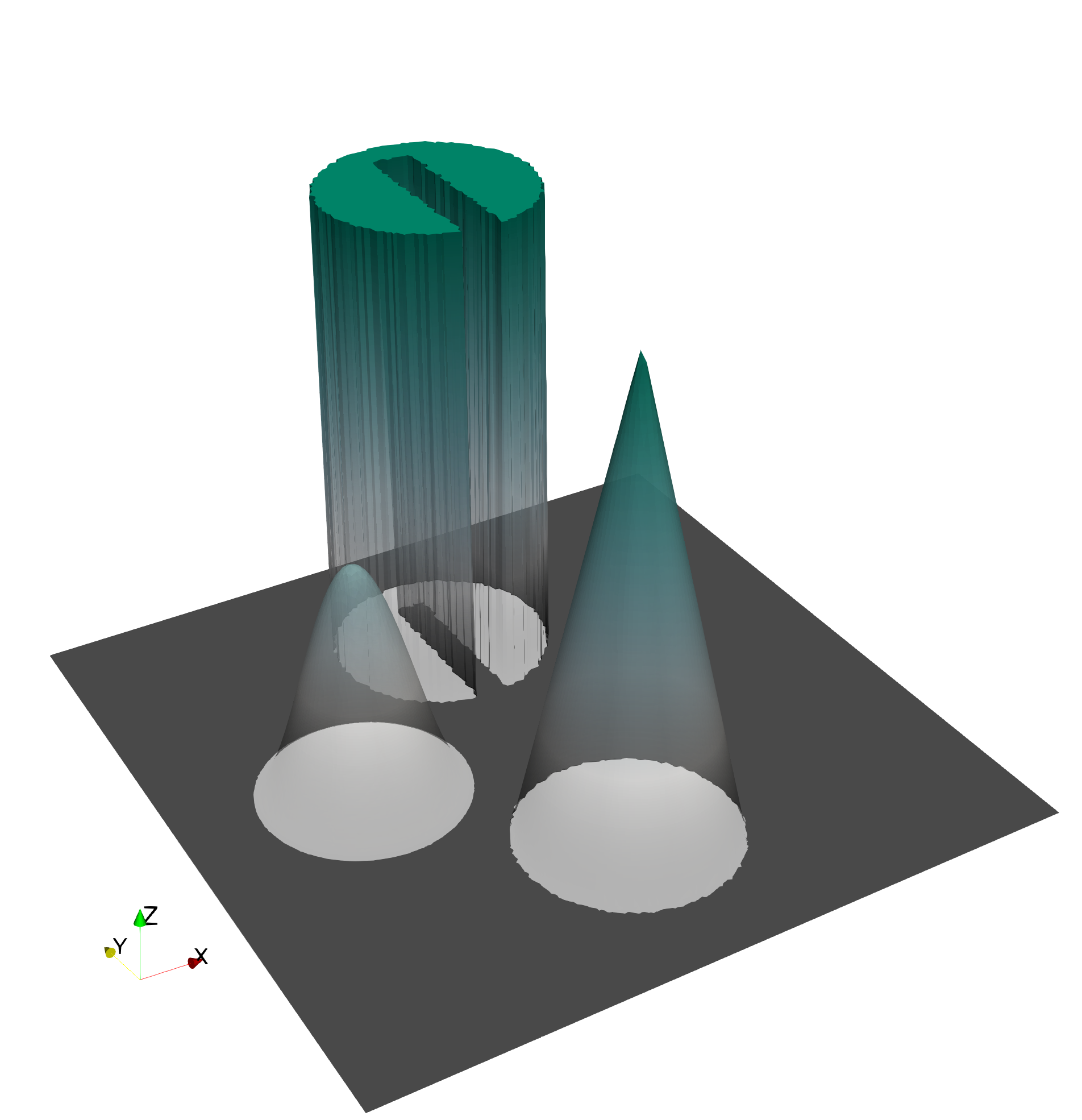
Refer to caption
(a) Exact solution.
Refer to caption
(b) p=0p=0.
Refer to caption
(c) p=1p=1.
Refer to caption
Refer to caption
(d) p=2p=2.
Refer to caption
(e) p=3p=3.
Refer to caption
(f) p=4p=4.
Figure 3: HDG solutions for the solid body rotation benchmark for different polynomial orders at end time tend=2​πt_{\mathrm{end}}=2\pi.
Refer to caption
(a) Exact solution.
Refer to caption
(b) p=0p=0.
Refer to caption
(c) p=1p=1.
Refer to caption
Refer to caption
(d) p=2p=2.
Refer to caption
(e) p=3p=3.
Refer to caption
(f) p=4p=4.
Figure 4: DG solutions for the solid body rotation benchmark for different polynomial orders at end time tend=2​πt_{\mathrm{end}}=2\pi.
Figure 5: Cross-sections of the DG solutions for the solid body rotation benchmark with p=3p=3 at end time tend=2​πt_{\mathrm{end}}=2\pi.

Our previous work in series was concerned with the same model problem (1) and the same linear flux (2); however, an unhybridized discontinuous Galerkin discretization with explicit strong stability preserving Runge–Kutta methods was used—in contrast to a HDG discretization and diagonally implicit Runge-Kutta schemes utilized in the current study. To make both implementations comparable, we implemented a variant of the DG solver that incorporates the DIRK schemes and computes the solid body rotation benchmark proposed by LeVeque [49] and used in [35] to investigate the performance of slope limiters. The initial solution consists of a slotted cylinder, a sharp cone, and a smooth hump (see Fig. 3(a)) placed in a square domain Ω=(0,1)2\Omega=(0,1)^{2} with velocity field 𝐮⁡(𝐱)=[0.5−x2,x1−0.5]T\mathbf{u}(\mathbf{x})={[0.5-x^{2},x^{1}-0.5]}^{\mathrm{T}} producing a full counterclockwise rotation of the initial scene over time interval J=(0,2​π)J=(0,2\pi). With r=0.0225r=0.0225 and G⁡(𝐱,𝐱0)≔10.15​‖𝐱−𝐱0‖2G(\mathbf{x},\mathbf{x}_{0})\coloneqq\frac{1}{0.15}\|\mathbf{x}-\mathbf{x}_{0}\|_{2}, we choose homogeneous Dirichlet boundary conditions cD=0c_{\mathrm{D}}=0 and right-hand-side function ξ=0\xi=0 with initial data satisfying

c0​(𝐱)={1if   (x1−0.5)2+(x2−0.75)2≤r  ∧(x1≤0.475∨x1≥0.525∨x2≥0.85)  (slotted cylinder)1−G⁡(𝐱,[0.5,0.25]T)if(x1−0.5)2+(x2−0.25)2≤r(sharp cone)14​(1+cos⁡(π​G​(𝐱,[0.25,0.5]T))CLOSEif(x1−0.25)2+(x2−0.5)2≤r(smooth hump)0otherwise}c^{0}(\mathbf{x})=\left\{\begin{array}[]{lll}1&\quad\text{if}\quad\parbox{124.20021pt}{$(x^{1}-0.5)^{2}+(x^{2}-0.75)^{2}\leq r$\\ $\land\;(x^{1}\leq 0.475\lor x^{1}\geq 0.525\lor x^{2}\geq 0.85)$}&\mbox{(slotted cylinder)}\\ 1-G(\mathbf{x},{[0.5,0.25]}^{\mathrm{T}})&\quad\text{if}\quad(x^{1}-0.5)^{2}+(x^{2}-0.25)^{2}\leq r&\mbox{(sharp cone)}\\ \frac{1}{4}(1+\cos(\pi G(\mathbf{x},{[0.25,0.5]}^{\mathrm{T}}))&\quad\text{if}\quad(x^{1}-0.25)^{2}+(x^{2}-0.5)^{2}\leq r&\mbox{(smooth hump)}\\ 0&\quad\text{otherwise}&\end{array}\right\}

An unstructured mesh generated by MATLAB’s initmesh with maximum element size h=2−6h=2^{-6} is used resulting in 14006 elements and 320 time steps.

‖ch​(tend)−c0‖L2​(Ω)\|c_{h}(t_{\mathrm{end}})-c^{0}\|_{L^{2}(\Omega)} runtime [s][s]
pp DG HDG DG HDG
0 1.87e-01 2.35e-01 27.1 39.8
1 7.25e-02 7.78e-02 157 218
2 5.53e-02 5.44e-02 797 717
3 4.02e-02 4.13e-02 3980 3166
4 4.16e-02 4.18e-02 10996 7199
Hardware / software details
CPU Intel Core-i7 4790 (Haswell)
RAM 32 GBytes
MATLAB R2017a
Table 5: Comparison of L2L^{2}-errors for the solid body rotation benchmark (cf. Sec. 5.2) at end time tend=2​πt_{\mathrm{end}}=2\pi (using initial data as the exact solution) and runtimes for DG and HDG solvers (left). Details of the employed hardware and software (right).

Figures 3 and 4 show the computed solution at end time tend=2​πt_{\mathrm{end}}=2\pi for different polynomial degrees. We chose a color map (inspired by [50]) that emphasizes violations of the discrete maximum principle: in the range [0,1][0,1] we have a color gradient from black via white to green; values in the range [−0.1,0)∪(1,1.1][-0.1,0)\cup(1,1.1] are colored red, and values in (−∞,−0.1)∪(1.1,+∞)(-\infty,-0.1)\cup(1.1,+\infty) are colored yellow. To make oscillations in the bottom range better visible, we gradually reduce the opacity from above to zero. Figure 5 presents intersection lines for p=3p=3.

Clearly, the lowest-order approximation is unusable for this kind of problem in both implementations with numerical diffusion killing off most (DG) or all (HDG) of the variability of the solution. For p>0p>0, solutions from HDG and DG are in good agreement for all approximation orders. This finding is substantiated by the intersection lines in Fig. 5 and the L2L^{2}-errors shown in Table 5 exhibiting only minor differences between both discretizations. However, also clearly visible are severe violations of the discrete maximum principles and oscillations in the wake of cylinder and cone, which do not become less pronounced with increasing approximation order. This type of behavior can be alleviated using slope limiters as shown in our previous work [35], where a post-processing step in each time level restricted the updated solution at the vertices to the bounds provided by the mean values of the adjacent elements. Unfortunately, designing slope limiters for implicit time stepping methods is not a trivial task and lies out of scope of this work.

When comparing the runtimes for both discretizations in Table 5, it becomes clear that the static condensation outlined in Sec. 3.4 becomes advantageous especially for higher approximation orders making HDG a superior approach for time-implicit high-order discretizations.

5.3 Performance analysis

hmax=2−4h_{\mathrm{max}}=2^{-4} (K=872)(K=872) hmax=2−6h_{\mathrm{max}}=2^{-6} (K=14006)(K=14006)
runtime assembly step solver step runtime assembly step solver step
pp 𝐆\mathbfsf{G} 𝐒\mathbfsf{S} 𝐋−𝟏\mathbfsf{L}^{-1} λ\lambda 𝐆\mathbfsf{G} 𝐒\mathbfsf{S} 𝐋−𝟏\mathbfsf{L}^{-1} λ\lambda
0 0.641 0.181 (28.2%\%) 0.047 (7.3%\%) 1.156 0.367 (31.7%\%) 0.617 (53.4%\%)
18.2%\% 8.3%\% 25.5%\% 61.7%\% 13.4%\% 19.6%\% 4.5%\% 91.9%\%
1 0.919 0.351 (38.2%\%) 0.278 (30.3%\%) 6.698 1.820 (27.2%\%) 4.674 (69.8%\%)
29.3%\% 17.9%\% 33.1%\% 59.0%\% 42.6%\% 29.3%\% 23.8%\% 71.2%\%
2 1.818 0.655 (36.0%\%) 0.852 (46.9%\%) 21.945 6.271 (28.6%\%) 15.491 (70.6%\%)
41.5%\% 21.4%\% 34.5%\% 56.0%\% 55.8%\% 31.0%\% 25.3%\% 66.1%\%
3 5.627 3.079 (54.7%\%) 2.353 (41.8%\%) 100.089 53.218 (53.2%\%) 46.688 (46.6%\%)
72.2%\% 15.6%\% 33.1%\% 53.7%\% 79.2%\% 17.0%\% 26.5%\% 60.2%\%
4 10.159 6.273 (61.7%\%) 3.685 (36.3%\%) 230.148 151.809 (66.0%\%) 78.151 (34.0%\%)
80.7%\% 12.3%\% 27.3%\% 53.9%\% 88.2%\% 9.9%\% 26.8%\% 56.6%\%
Table 6: Runtime distribution for 10 time steps of the solid body rotation benchmark (cf. Sec. 5.2) without initialization tasks (i.e., only time stepping loop) measured using MATLAB’s profiler. We compare different mesh sizes and approximation orders with runtimes given in seconds. Percentages for assembly and solvers are relative to the runtime of the time stepping loop, percentages for the assembly of 𝐆\mathbfsf{G} and 𝐒\mathbfsf{S} (cf. secs. 4.3.2 and 4.3.1) are relative to assembly runtime, and percentages for inversion of 𝐋\mathbfsf{L} (cf. sec. 3.4) and solving (32) for λ\lambda are relative to solver step runtimes. Details on the employed hardware and software are given in Table 5 (right).

A major advantage of the hybridized DG method is the fact that the globally coupled linear equation system resulting from the discretization is relatively compact and easy to solve (see Sec. 3.4 for details). To illustrate this, we present some performance results that show the runtime distribution among the different steps of the code. We disregard pre-processing and initialization tasks as these are only performed once and consider ten time steps of the solid body rotation benchmark presented in Sec. 5.2. Using MATLAB’s profiler to determine the runtime share of each instruction we see — just as expected — that the linear solvers together with the assembly of the time-dependent block matrices, particularly 𝐆\mathbfsf{G} and 𝐒\mathbfsf{S}, are responsible for the majority of the computation time. Table 6 shows the runtime shares for the most expensive parts of the code.

First of all, the overall runtime clearly increases with mesh size and polynomial approximation order simply due to the increasing number of degrees of freedom. More intriguing is the fact that the assembly step becomes more dominant than the linear system solves with the increasing polynomial degree. The primary reason for this is the assembly of matrices 𝐆𝐦\mathbfsf{G}^{m}, which do not only grow in size due to the increasing number of degrees of freedom but also require a loop over all quadrature points (see Sec. 4.3.1 for details). With the order of the quadrature rule (and thus the number of quadrature points) increasing with the polynomial degree, the computational complexity of this operation grows quickly. Nevertheless, the total runtime increase for higher polynomial approximation orders is not as pronounced as for the unhybridized DG solver as shown in Sec. 5.2.

In contrast to the shift in the assembly step, the runtime distribution between the block-wise inversion of 𝐋\mathbfsf{L} and solving (32) is very similar throughout all approximation orders and different mesh sizes. We would like to point out that the local solves with 𝐋−𝟏\mathbfsf{L}^{-1} are element-local and thus could be easily parallelized with virtually perfect scaling.

6 Register of routines

In this section, the routines added since the first two papers in series [34, 35] are presented in form of a two-part list: first, the scripts implementing the solution algorithm in the order they are executed followed by the alphabetically ordered list of assembly and integration routines used in the solution algorithm. In the code available on GitHub [37], all routines check for correctly provided function arguments using MATLAB / GNU Octave’s validateattributes excluded here for brevity.

All data that is needed throughout the entire algorithm (e. g., mesh data structures, pre-computed reference blocks, etc.) are passed between steps in a struct always called problemData. In all routines, the argument g is a struct containing information about the triangulation. Input parameter N is the number of degrees of freedom for the 2D polynomials φh\varphi_{h}, and Nmu is the number of degrees of freedom for the 1D polynomials μh\mu_{h}. Parameter qOrd is the order of the quadrature rule, and basesOnQuad is a struct that contains basis functions φh\varphi_{h} and μh\mu_{h} evaluated in quadrature points of the reference element T^\hat{T}, edges E^n\hat{E}_{n} of the reference element, and reference interval [0,1][0,1]. In the time stepping routines, nStep always refers to the current time step index nn and nSubStep to the current Runge-Kutta stage ii (cf. Sec. 3.3).

6.1 Solution algorithm

problemData = configureProblem(problemData) is executed first and fills the problemData-struct with all basic configuration options. Problem parameters are to be modified inside this routine.

function problemData = configureProblem(problemData)
%% Parameters.
% Choose testcase
problemData = setdefault(problemData, 'testcase', 'solid_body');
% Mark run as convergence test (enforces Friedrichs-Keller triangulation)
problemData = setdefault(problemData, 'isConvergence', false);
% Maximum edge length of triangle
problemData = setdefault(problemData, 'hmax', 2^-6);
% Local polynomial approximation order (0 to 4)
problemData = setdefault(problemData, 'p', 2);
% Order of Runge-Kutta method
problemData = setdefault(problemData, 'ordRK', min(problemData.p + 1, 4));
% Order of quadrature rule
problemData = setdefault(problemData, 'qOrd', 2*problemData.p + 1);
% Load testcase
problemData = getTestcase(problemData, problemData.testcase);
% Visualization settings
problemData = setdefault(problemData, 'isVisGrid', false); % visualization of grid
problemData = setdefault(problemData, 'isVisSol', true); % visualization of solution
problemData = setdefault(problemData, 'outputFrequency', 50); % no visualization of every timestep
problemData = setdefault(problemData, 'outputBasename', ['output' filesep 'hdg_advection']);
problemData = setdefault(problemData, 'outputTypes', { 'vtk', 'tec' }); % Type of visualization files
% HDG stabilization parameter
problemData = setdefault(problemData, 'stab', 1.0);
% Enable blockwise local solves and specify block size
problemData = setdefault(problemData, 'isBlockSolve', true);
problemData = setdefault(problemData, 'blockSolveSize', 2^(5 - problemData.p));
%% Domain and triangulation configuration.
% Triangulate unit square using pdetool (if available or Friedrichs-Keller otherwise).
if ~problemData.isConvergence && license('checkout','PDE_Toolbox')
problemData.generateGridData = @(hmax) domainPolygon([0 1 1 0], [0 0 1 1], hmax);
else
fprintf('PDE_Toolbox␣not␣available.␣Using␣Friedrichs-Keller␣triangulation.\n');
problemData.generateGridData = @domainSquare;
end % if
end % function

problemData = preprocessProblem(problemData) performs all pre-processing tasks and one-time computations prior to the projection of the initial data and the time stepping loop. This includes mesh generation, evaluation of basis functions in quadrature points, computation of blocks for the reference elements and edges, and assembly of time-independent block matrices.

function problemData = preprocessProblem(problemData)
%% Triangulation.
problemData.g = problemData.generateGridData(problemData.hmax);
if problemData.isVisGrid, visualizeGrid(problemData.g); end
%% Globally constant parameters.
problemData.K = problemData.g.numT; % number of triangles
problemData.N = nchoosek(problemData.p + 2, problemData.p); % number of local DOFs
problemData.Nmu = problemData.p + 1; % number of local DOFs on Faces
problemData.dt = problemData.tEnd / problemData.numSteps;
% [K x 3] arrays that mark local edges (E0T) or vertices (V0T) that are
% interior or have a certain boundary type.
problemData.g.markE0Tint = problemData.generateMarkE0Tint(problemData.g);
problemData.g.markE0Tbdr = problemData.generateMarkE0Tbdr(problemData.g);
% Precompute some repeatedly evaluated fields
problemData.g = computeDerivedGridData(problemData.g);
%% Configuration output.
fprintf('Computing␣with␣polynomial␣order␣%d␣(%d␣local␣DOFs)␣on␣%d␣triangles␣and␣%d␣edges.\n', ...
problemData.p, problemData.N, problemData.K, problemData.g.numE)
qOrd = problemData.qOrd;
N = problemData.N;
Nmu = problemData.Nmu;
%% Lookup table for basis function.
problemData.basesOnQuad = computeBasesOnQuad(N, struct, [qOrd, qOrd + 1]);
problemData.basesOnQuad = computeBasesOnQuadEdge(Nmu, problemData.basesOnQuad, [qOrd, qOrd + 1]);
%% Computation of matrices on the reference triangle.
problemData.hatM = integrateRefElemPhiPhi(N, problemData.basesOnQuad, qOrd);
hatMmu = integrateRefEdgeMuMu(Nmu, problemData.basesOnQuad, qOrd);
problemData.hatRmu = integrateRefEdgePhiIntMu([N, Nmu], problemData.basesOnQuad, qOrd);
hatRphi = integrateRefEdgePhiIntPhiInt(N, problemData.basesOnQuad, qOrd);
problemData.hatG = integrateRefElemDphiPhiPerQuad(N, problemData.basesOnQuad, qOrd);
problemData.hatS = integrateRefEdgePhiIntMuPerQuad([N, Nmu], problemData.basesOnQuad, qOrd);
%% Assembly of time-independent global matrices.
problemData.globMphi = assembleMatElemPhiPhi(problemData.g, problemData.hatM);
problemData.globRmu = assembleMatEdgePhiIntMu(problemData.g, problemData.g.markE0Tint, ...
problemData.hatRmu);
problemData.globRphi = assembleMatEdgePhiIntPhiInt(problemData.g, problemData.g.markE0Tint, hatRphi);
problemData.globMmuBar = assembleMatEdgeMuMu(problemData.g, problemData.g.markE0Tint, hatMmu);
problemData.globMmuTilde = assembleMatEdgeMuMu(problemData.g, problemData.g.markE0Tbdr, hatMmu);
problemData.globP = problemData.stab .* problemData.globMmuBar + problemData.globMmuTilde;
problemData.globT = problemData.globRmu';
end␣%␣function'

problemData = initializeProblem(problemData) projects initial data c0c^{0} and visualizes the initial state.

function problemData = initializeProblem(problemData)
problemData.isFinished = false;
%% Initial data on elements and faces
if ~problemData.isStationary
problemData.cDisc = projectFuncCont2DataDisc(problemData.g, problemData.c0Cont, problemData.qOrd, ...
problemData.hatM, problemData.basesOnQuad);
fprintf('L2␣error␣w.r.t.␣the␣initial␣condition:␣%g\n', computeL2Error(problemData.g, ...
problemData.cDisc, problemData.c0Cont, problemData.qOrd + 1, problemData.basesOnQuad));
%% visualization of inital condition.
if problemData.isVisSol
cLgr = projectDataDisc2DataLagr(problemData.cDisc);
visualizeDataLagr(problemData.g, cLgr, 'u_h', problemData.outputBasename,0,problemData.outputTypes)
end
fprintf('Starting␣time␣integration␣from␣0␣to␣%g␣using␣time␣step␣size␣%g␣(%d␣steps).\n', ...
problemData.tEnd, problemData.dt, problemData.numSteps)
end % if
end % function

problemData = preprocessStep(problemData, nStep) is the first step in each iteration of the time stepping loop and applies mass matrix 𝐌φ\mathbfsf{M}_{\varphi} to solution vector 𝐂n\mathbf{C}^{n} required in each stage of the DIRK schemes.

function problemData = preprocessStep(problemData, nStep)
if ~problemData.isStationary
problemData.globMcDisc = problemData.globMphi * reshape(problemData.cDisc',␣[],␣1);
end␣%␣if
end␣%␣function'

problemData = solveStep(problemData, nStep) is the main routine of the time stepping loop and determines Runge-Kutta coefficients before initiating sub-stepping to carry out the Runge-Kutta stages.

function problemData = solveStep(problemData, nStep)
if problemData.isStationary
problemData.t = 0;
else
% Obtain Runge-Kutta rule and initialize solution vectors
[problemData.t, problemData.A, problemData.b] = rungeKuttaImplicit(problemData.ordRK, ...
problemData.dt, (nStep - 1) * problemData.dt);
problemData.cDiscRK = cell(length(problemData.t), 1);
end % if
% Carry out RK steps
problemData.isSubSteppingFinished = false;
problemData = iterateSubSteps(problemData, nStep);
end % function

problemData = preprocessSubStep(problemData, nStep, nSubStep) is the main assembly routine of the current Runge-Kutta stage, where velocity function 𝐮\mathbf{u} is evaluated at quadrature points of all edges, inflow and outflow boundaries are determined, and all time-dependent block matrices and right-hand-side vectors are built.

function problemData = preprocessSubStep(problemData, nStep, nSubStep)
% Select time level for current Runge-Kutta stage
t = problemData.t(nSubStep);
cDCont = @(x1, x2) problemData.cDCont(t, x1 ,x2);
u1Cont = @(x1, x2) problemData.u1Cont(t, x1, x2);
u2Cont = @(x1, x2) problemData.u2Cont(t, x1, x2);
fCont = @(x1,x2) problemData.fCont(t, x1, x2);
% Evaluate normal advection velocity on every edge.
uNormalQ0E0T = computeFuncContNuOnQuadEdge(problemData.g, u1Cont, u2Cont, problemData.qOrd);
% Determine inflow- and outflow edges
[~, W] = quadRule1D(problemData.qOrd);
markE0TbdrOut = problemData.g.markE0Tbdr & sum(bsxfun(@times, reshape(W,1,1,[]), uNormalQ0E0T), 3) > 0;
markE0TbdrIn = problemData.g.markE0Tbdr & ~markE0TbdrOut;
% Assemble source term.
problemData.globH = problemData.globMphi * reshape(projectFuncCont2DataDisc(problemData.g, fCont, ...
problemData.qOrd, problemData.hatM, problemData.basesOnQuad)',␣[],␣1);
%␣Assemble␣element␣integral␣contributions.
problemData.globG␣=␣assembleMatElemDphiPhiFuncContVec(problemData.g,␣problemData.hatG,␣...
␣␣␣␣␣␣␣␣␣␣␣␣␣␣␣␣␣␣␣␣␣␣␣␣u1Cont,␣u2Cont,␣problemData.qOrd);
%␣Assemble␣flux␣on␣interior␣and␣outflow␣edges
problemData.globS␣=␣assembleMatEdgePhiIntMuVal(problemData.g,␣problemData.g.markE0Tint|markE0TbdrOut,...
␣␣␣␣␣␣␣␣␣␣␣␣␣␣␣␣␣␣␣␣␣␣␣␣problemData.hatS,␣uNormalQ0E0T);
problemData.globKmuOut␣=␣assembleMatEdgePhiIntMu(problemData.g,␣markE0TbdrOut,␣problemData.hatRmu)';
% Assemble inflow boundary conditions.
cQ0E0T = computeFuncContOnQuadEdge(problemData.g, cDCont, problemData.qOrd);
problemData.globFphiIn = assembleVecEdgePhiIntVal(problemData.g, markE0TbdrIn, ...
cQ0E0T .* uNormalQ0E0T, problemData.N, problemData.basesOnQuad);
problemData.globKmuIn = assembleVecEdgeMuFuncCont(problemData.g, markE0TbdrIn, ...
cDCont, problemData.basesOnQuad, problemData.qOrd);
end % function

problemData = solveSubStep(problemData, nStep, nSubStep) builds and solves the linear systems described in Sec. 3.4 for the current Runge-Kutta stage.

function problemData = solveSubStep(problemData, nStep, nSubStep)
K = problemData.K;
N = problemData.N;
if problemData.isStationary
matL = - problemData.globG{1} - problemData.globG{2} + problemData.stab * problemData.globRphi;
vecQ = problemData.globH - problemData.globFphiIn;
matM = problemData.globS - problemData.stab * problemData.globRmu;
else
dtA = problemData.dt * problemData.A;
cDiscRkRHS = zeros(K * N, 1);
for i = 1 : nSubStep - 1
cDiscRkRHS = cDiscRkRHS + dtA(nSubStep, i) .* problemData.cDiscRK{i};
end
matLbar = - problemData.globG{1} - problemData.globG{2} + problemData.stab * problemData.globRphi;
matL = problemData.globMphi + dtA(nSubStep, nSubStep) .* matLbar;
vecBphi = problemData.globH - problemData.globFphiIn;
vecQ = problemData.globMcDisc + dtA(nSubStep, nSubStep) * vecBphi + cDiscRkRHS;
matMbar = problemData.globS - problemData.stab * problemData.globRmu;
matM = dtA(nSubStep, nSubStep) .* matMbar;
end % if
%% Computing local solves
if problemData.isBlockSolve
matLinv = blkinv(matL, problemData.blockSolveSize * N);
LinvQ = matLinv * vecQ;
LinvM = matLinv * matM;
else
LinvQ = matL \ vecQ;
LinvM = matL \ matM;
end % if
%% Solving global system for lambda
matN = - problemData.stab * problemData.globT - problemData.globKmuOut ;
matP = problemData.globP;
lambdaDisc = (-matN * LinvM + matP) \ (problemData.globKmuIn - matN * LinvQ);
%% Reconstructing local solutions from updated lambda
problemData.cDisc = LinvQ - LinvM * lambdaDisc;
if ~problemData.isStationary
problemData.cDiscRK{nSubStep} = vecBphi - matLbar * problemData.cDisc - matMbar * lambdaDisc;
end % if
problemData.cDisc = reshape(problemData.cDisc, N, K)';
end␣%␣function'

problemData = postprocessSubStep(problemData, nStep, nSubStep) determines whether ...SubStep-routines must be executed once more to carry out the remaining Runge-Kutta stages or if control has to be returned to function solveStep.

function problemData = postprocessSubStep(problemData, nStep, nSubStep)
problemData.isSubSteppingFinished = problemData.isStationary || nSubStep >= length(problemData.t);
end % function

problemData = postprocessStep(problemData, nStep) checks if all time integration steps have been carried out or if another iteration of the time stepping loop is required.

function problemData = postprocessStep(problemData, nStep)
problemData.isFinished = problemData.isStationary || nStep >= problemData.numSteps;
end % function

problemData = outputStep(problemData, outputStep) writes visualization output files for the updated solution.

function problemData = outputStep(problemData, nStep)
%% visualization
if problemData.isVisSol && mod(nStep, problemData.outputFrequency) == 0
cLagrange = projectDataDisc2DataLagr(problemData.cDisc);
visualizeDataLagr(problemData.g, cLagrange, 'u_h', problemData.outputBasename, ...
nStep, problemData.outputTypes);
end % if
end % function

problemData = postprocessProblem(problemData) is executed after termination of the time stepping loop and computes the L2L^{2}-error of the solution if the analytical solution is provided.

function problemData = postprocessProblem(problemData)
%% Visualization
if problemData.isVisSol
cLagrange = projectDataDisc2DataLagr(problemData.cDisc);
visualizeDataLagr(problemData.g, cLagrange, 'u_h', problemData.outputBasename, ...
problemData.numSteps, problemData.outputTypes);
end % if
fprintf('Finished␣simulation␣at␣t_end␣=␣%g\n', problemData.tEnd);
%% Error evaluation
if isfield(problemData, 'cCont')
problemData.error = computeL2Error(problemData.g, problemData.cDisc, ...
@(x1, x2) problemData.cCont(problemData.tEnd, x1, x2), problemData.qOrd, problemData.basesOnQuad);
fprintf('L2␣error␣w.r.t.␣the␣analytical␣solution:␣%g\n', problemData.error);
else
problemData.error = computeL2Error(problemData.g, problemData.cDisc, ...
problemData.c0Cont, problemData.qOrd, problemData.basesOnQuad);
fprintf('L2␣error␣w.r.t.␣the␣initial␣condition:␣%g\n', problemData.error);
end % if
end % function

6.2 Helper routines

ret = assembleMatEdgeMuMu(g, markE0T, refEdgeMuMu) assembles mass-matrices 𝐌¯μ\mathbfsf{\mkern 1.5mu\overline{\mkern-1.5muM\mkern-1.5mu}\mkern 1.5mu}_{\mu} and 𝐌~μ\tilde{\mathbfsf{M}}_{\mu} for the edge-based basis functions μh\mu_{h} as described in Sec. 4.3.4. Array markE0T plays the role of the Kronecker delta in the matrix definition by selecting the relevant edges for either matrix. refEdgeMuMu is the mass matrix 𝐌^μ\mathbfsf{\hat{M}}_{\mu} on the reference interval [0,1][0,1] computed by integrateRefEdgeMuMu.

function ret = assembleMatEdgeMuMu(g, markE0T, refEdgeMuMu)
Nmu = size(refEdgeMuMu, 1); Kedge = g.numE;
ret = sparse(Kedge * Nmu, Kedge * Nmu);
for n = 1 : 3
Kkn = g.areaE0T(:, n) .* markE0T(:, n) ;
ret = ret + kron(sparse(g.E0T(:, n), g.E0T(:, n), Kkn, Kedge, Kedge), refEdgeMuMu);
end % for
end % function

ret = assembleMatEdgePhiIntMu(g, markE0T, refEdgePhiIntMu) assembles matrices 𝐑μ\mathbfsf{R}_{\mu}, 𝐓\mathbfsf{T}, and 𝐊μ,out\mathbfsf{K}_{\mu,\mathrm{out}} as detailed in Sec. 4.3.3. As before, markE0T is used to select relevant edges, and refEdgePhiIntMu stores the pre-computed reference blocks 𝐑^μ\mathbfsf{\hat{R}}_{\mu} given by integrateRefEdgePhiIntMu.

function ret = assembleMatEdgePhiIntMu(g, markE0T, refEdgePhiIntMu)
K = g.numT; Kedge = g.numE;
[N, Nmu, ~, ~] = size(refEdgePhiIntMu);
ret = sparse(K * N, Kedge * Nmu);
for n = 1 : 3
for l = 1 : 2
Rkn = markE0T(:,n) .* g.markSideE0T(:, n, l) .* g.areaE0T(:, n);
ret = ret + kron(sparse(1 : K, g.E0T(:, n), Rkn, K, Kedge), refEdgePhiIntMu(:, :, n, l));
end % for
end % for
end % function

ret = assembleMatEdgePhiIntMuVal(g, markE0T, refEdgePhiIntMuPerQuad, valOnQuad) builds the global matrices 𝐒\mathbfsf{S} and 𝐒out\mathbfsf{S}_{\text{out}} given in Sec. 4.3.2. Both matrices are assembled at once by specifying all interior and outflow edges as markE0T. The reference blocks per quadrature point 𝐒^\mathbfsf{\hat{S}} are computed by integrateRefEdgePhiIntMuPerQuad and specified in the parameter refEdgePhiIntMuPerQuad. Parameter valOnQuad stores the normal velocity 𝐔𝝂\mathbf{U}_{\boldsymbol{\nu}} evaluated at the quadrature points of each edge.

function ret = assembleMatEdgePhiIntMuVal(g, markE0T, refEdgePhiIntMuPerQuad, valOnQuad)
K = g.numT; Kbar = g.numE;
[N, Nmu, ~, R] = size(refEdgePhiIntMuPerQuad{1});
ret = sparse(K*N, Kbar*Nmu);
for n = 1 : 3
RknTimesVal = sparse(K*N, Nmu);
markAreaE0T = markE0T(:, n) .* g.areaE0T(:, n);
for l = 1 : 2
markAreaSideE0T = markAreaE0T .* g.markSideE0T(:, n, l);
for r = 1 : R
RknTimesVal = RknTimesVal + kron(markAreaSideE0T .* valOnQuad(:, n, r), ...
refEdgePhiIntMuPerQuad{l}(:, :, n, r));
end % for r
end % for l
ret = ret + kronVec(sparse(1:K, g.E0T(:, n), ones(K, 1), K, Kbar), RknTimesVal);
end % for n
end % function

ret = assembleMatElemDphiPhiFuncContVec(g, refElemDphiPhiPerQuad, funcCont1, funcCont2, qOrd) assembles matrices 𝐆𝐦\mathbfsf{G}^{m} described in Sec. 4.3.1. Reference blocks 𝐆^\mathbfsf{\hat{G}} are provided in parameter refElemDphiPhiPerQuad and computed by integrateRefElemDphiPhiPerQuad. The two components of the continuous function in the integrand – here the velocity components – are given as function handles in funcCont1 and funcCont2, respectively.

function ret = assembleMatElemDphiPhiFuncContVec(g, refElemDphiPhiPerQuad, funcCont1, funcCont2, qOrd)
K = g.numT; [N, ~, R] = size(refElemDphiPhiPerQuad{1});
if nargin < 5, p = (sqrt(8*N+1)-3)/2; qOrd = max(2*p, 1); end
[Q1, Q2, ~] = quadRule2D(qOrd);
ret = { zeros(K*N, N), zeros(K*N,N) };
for r = 1 : R
valOnQuad1 = funcCont1(g.mapRef2Phy(1, Q1(r), Q2(r)), g.mapRef2Phy(2, Q1(r), Q2(r)));
ret{1} = ret{1} + kron(g.B(:,2,2) .* valOnQuad1, refElemDphiPhiPerQuad{1}(:, :, r)) ...
- kron(g.B(:,2,1) .* valOnQuad1, refElemDphiPhiPerQuad{2}(:, :, r));
valOnQuad2 = funcCont2(g.mapRef2Phy(1, Q1(r), Q2(r)), g.mapRef2Phy(2, Q1(r), Q2(r)));
ret{2} = ret{2} - kron(g.B(:,1,2) .* valOnQuad2, refElemDphiPhiPerQuad{1}(:, :, r)) ...
+ kron(g.B(:,1,1) .* valOnQuad2, refElemDphiPhiPerQuad{2}(:, :, r));
end % for
ret{1} = kronVec(speye(K,K), ret{1});
ret{2} = kronVec(speye(K,K), ret{2});
end % function

ret = assembleVecEdgeMuFuncCont(g, markE0T, funcCont, basesOnQuad, qOrd) builds the vector with Dirichlet data 𝐊μ,in\mathbf{K}_{\mu,\mathrm{in}} (cf. Sec. 4.3.5). Inflow edges are specified in markE0T, and Dirichlet data is specified as a function handle in funcCont.

function ret = assembleVecEdgeMuFuncCont(g, markE0T, funcCont, basesOnQuad, qOrd)
[Q, W] = quadRule1D(qOrd);
[R, Nmu] = size(basesOnQuad.mu{qOrd});
ret = zeros(g.numE, Nmu);
for n = 1 : 3
[Q1, Q2] = gammaMap(n, Q);
funcOnQuad = funcCont(g.mapRef2Phy(1, Q1, Q2), g.mapRef2Phy(2, Q1, Q2));
Kkn = markE0T(:, n) .* g.areaE0T(:,n);
ret(g.E0T(:, n), :) = ret(g.E0T(:, n), :) + (repmat(Kkn, 1, R) .* funcOnQuad) ...
* ( repmat(W',␣1,␣Nmu)␣.*␣basesOnQuad.mu{qOrd}␣);
end␣%␣for
ret␣=␣reshape(ret', [], 1);
end % function

invA = blkinv(A, blockSize) inverts a square block-diagonal matrix A built up from blocks of size n×nn\times n, which is used to compute 𝐋−𝟏\mathbfsf{L}^{-1} as described in Sec. 3.4. To improve the computational performance of this method, the inversion is performed using a blocking-technique where a pre-specified number of diagonal blocks are inverted together. Parameter blockSize specifies the blocking size and must be a multiple of nn.

function invA = blkinv(A, blockSize)
n = size(A,1);
numBlocks = ceil(n / blockSize);
idxEnd = (numBlocks - 1) * blockSize;
idxs = mat2cell(1 : idxEnd, 1, ones(1, numBlocks - 1) * blockSize);
cellA = cellfun(@(X) A(X, X), idxs, 'UniformOutput', false);
cellInvA = cellfun(@(X) inv(X), cellA, 'UniformOutput', false);
invA = blkdiag(cellInvA{:}, inv(A(idxEnd + 1 : end, idxEnd + 1 : end)));
end % function

basesOnQuadEdge = computeBasesOnQuadEdge(N, basesOnQuadEdge, requiredOrders) evaluates edge basis function μh\mu_{h} at the quadrature points of the reference interval [0,1][0,1]. Parameter basesOnQuadEdge is a (possibly empty) struct to which the computed fields mu and thetaMu (the latter corresponding to μ^∘β^k​n\hat{\mu}\circ\hat{\beta}_{kn}) are added. The quadrature orders can be optionally specified in requiredOrders and with defaults equal to 2​p2p and 2​p+12p+1.

function basesOnQuadEdge = computeBasesOnQuadEdge(N, basesOnQuadEdge, requiredOrders)
if nargin < 3
p = N - 1;
if p > 0
requiredOrders = [2*p, 2*p+1];
else
requiredOrders = 1;
end % if
end % if
basesOnQuadEdge.mu = cell(max(requiredOrders),1);
basesOnQuadEdge.thetaMu = cell(max(requiredOrders),1);
for it = 1 : length(requiredOrders)
ord = requiredOrders(it);
[Q, ~] = quadRule1D(ord);
R = length(Q);
basesOnQuadEdge.mu{ord} = zeros(R, N);
for i = 1 : N
basesOnQuadEdge.mu{ord}(:, i) = phi1D(i, Q);
end
basesOnQuadEdge.thetaMu{ord} = zeros(R, N, 2);
basesOnQuadEdge.thetaMu{ord}(:, :, 1) = basesOnQuadEdge.mu{ord};
basesOnQuadEdge.thetaMu{ord}(:, :, 2) = flipud(basesOnQuadEdge.mu{ord});
end % for
end % function

g = computeDerivedGridData(g) enriches grid data structure g by an additional K×3×2K\times 3\times 2 field markSideE0T that marks for each element-local edge, whether the element has local index 1 or 2 at the edge thus providing a way to determine ll in the mapping κ\kappa (cf. eq. (6)) for given element TkT_{k} and edge Ek​n=Ek¯E_{kn}=E_{\bar{k}}.

function g = computeDerivedGridData(g)
g.markSideE0T = true(g.numT, 3, 2);
for n = 1 : 3
% Mark element to have local id 1 or 2 at the given edge
g.markSideE0T(:, n, 1) = g.T0E(g.E0T(:, n), 2) ~= (1:g.numT)';
␣␣g.markSideE0T(:,␣n,␣2)␣=␣~g.markSideE0T(:,␣n,␣1);
end␣%␣for
end␣%␣function'

ret = computeFuncContOnQuadEdge(g, funcCont, qOrd) evaluates a given function handle funcCont in all quadrature points of all edges. This is used to determine the Dirichlet boundary data cDc_{\mathrm{D}} before multiplying it with the normal velocity and assembling 𝐅φ,in\mathbf{F}_{\varphi,\mathrm{in}} in routine assembleVecEdgePhiIntVal.

function ret = computeFuncContOnQuadEdge(g, funcCont, qOrd)
K = g.numT; [Q, W] = quadRule1D(qOrd);
ret = zeros(K, 3, length(W));
for n = 1 : 3
[Q1, Q2] = gammaMap(n, Q);
ret(:, n, :) = funcCont(g.mapRef2Phy(1, Q1, Q2), g.mapRef2Phy(2, Q1, Q2));
end % for
end % function

problemData = getTestcase(problemData, testcase) defines initial and boundary data as well as the analytical solution, if available, for test cases given in Sec. 5. To shorten the presentation, the actual definitions are omitted here but can be found in GitHub [37].

function problemData = getTestcase(problemData, testcase)
switch testcase
case 'solid_body'
% LeVeque's solid body rotation
case 'stationary'
% Stationary analytical example
case 'transient_ode'
% Transient ODE example
case 'transient'
% Transient analytical example
otherwise
error('Invalid␣testcase␣"%s".', testcase);
end % switch
fprintf('Loaded␣testcase␣"%s".\n', testcase);
% Time stepping parameters
problemData = setdefault(problemData, 'numSteps', numSteps);
problemData = setdefault(problemData, 'tEnd', tEnd);
problemData = setdefault(problemData, 'isStationary', isStationary);
% Store defined functions in struct
problemData = setdefault(problemData, 'c0Cont', c0Cont);
problemData = setdefault(problemData, 'fCont', fCont);
problemData = setdefault(problemData, 'u1Cont', u1Cont);
problemData = setdefault(problemData, 'u2Cont', u2Cont);
problemData = setdefault(problemData, 'cDCont', cDCont);
if isAnalytical, problemData = setdefault(problemData, 'cCont', cCont); end
% Specify boundary conditions
problemData = setdefault(problemData, 'generateMarkE0Tint', @(g) g.idE0T == 0);
problemData = setdefault(problemData, 'generateMarkE0Tbdr', @(g) g.idE0T ~= 0);
end % function

ret = integrateRefEdgeMuMu(N, basesOnQuadEdge, qOrd) computes reference blocks 𝐌^μ\mathbfsf{\hat{M}}_{\mu} (see Sec. 4.3.4).

function ret = integrateRefEdgeMuMu(N, basesOnQuad, qOrd)
if nargin < 3, p = N-1; qOrd = 2*p+1; end
[~, W] = quadRule1D(qOrd);
ret = zeros(N, N); % [N x N]
for i = 1 : N
for j = 1 : N
ret(i, j) = sum( W'␣.*␣basesOnQuad.mu{qOrd}(:,i)␣.*␣basesOnQuad.mu{qOrd}(:,j)␣);
␣␣end␣%␣for
end␣%␣for
end␣%␣function'

ret = integrateRefEdgePhiIntMu(N, basesOnQuad, qOrd) computes reference blocks 𝐑^μ\mathbfsf{\hat{R}}_{\mu} (see Sec. 4.3.3).

function ret = integrateRefEdgePhiIntMu(N, basesOnQuad, qOrd)
if nargin < 3, p = (sqrt(8*N(1)+1)-3)/2; qOrd = 2*p+1; end
[~, W] = quadRule1D(qOrd);
ret = zeros(N(1), N(2), 3, 2); % [N(1) x N(2) x 3 x 2]
for n = 1 : 3
for i = 1 : N(1)
for j = 1 : N(2)
ret(i, j, n, 1) = W * (basesOnQuad.phi1D{qOrd}(:, i, n) .* basesOnQuad.mu{qOrd}(:, j) );
ret(i, j, n, 2) = W * (basesOnQuad.phi1D{qOrd}(:, i, n) .* basesOnQuad.thetaMu{qOrd}(:, j, 2) );
end % for
end % for
end % for
end % function

ret = integrateRefEdgePhiIntMuPerQuad(N, basesOnQuad, qOrd) computes reference blocks 𝐒^\mathbfsf{\hat{S}} (see Sec. 4.3.2).

function ret = integrateRefEdgePhiIntMuPerQuad(N, basesOnQuad, qOrd)
if nargin < 3, p = (sqrt(8*N+1)-3)/2; qOrd = 2*p+1; end
[~, W] = quadRule1D(qOrd); R = length(W);
ret = { zeros(N(1), N(2), 3, R); zeros(N(1), N(2), 3, R) };
for n = 1 : 3
for i = 1 : N(1)
for j = 1 : N(2)
ret{1}(i, j, n, :) = W(:) .* basesOnQuad.phi1D{qOrd}(:, i, n) ...
.* basesOnQuad.mu{qOrd}(:, j);
ret{2}(i, j, n, :) = W(:) .* basesOnQuad.phi1D{qOrd}(:, i, n) ...
.* basesOnQuad.thetaMu{qOrd}(:, j, 2);
end % for j
end % for i
end % for n
end % function

ret = integrateRefElemDphiPhiPerQuad(N, basesOnQuad, qOrd) computes reference blocks 𝐆^\mathbfsf{\hat{G}} (see Sec. 4.3.1).

function ret = integrateRefElemDphiPhiPerQuad(N, basesOnQuad, qOrd)
if nargin < 3, p = (sqrt(8*N+1)-3)/2; qOrd = max(2*p, 1); end
[~, ~, W] = quadRule2D(qOrd); R = length(W);
ret = { zeros(N, N, R); zeros(N, N, R) };
for i = 1 : N
for j = 1 : N
for m = 1 : 2
ret{m}(i, j, :) = W(:) .* basesOnQuad.phi2D{qOrd}(:, j) .* basesOnQuad.gradPhi2D{qOrd}(:, i, m);
end % for
end % for
end % for
end % function

[t, A, b, c] = rungeKuttaImplicit(ord, tau, t0) provides the Butcher tableau for DIRK schemes of orders one to four (see Sec. 3.3) with the order given in ord. The current time level is provided in t0, and the time step size is given in tau.

function [t, A, b, c] = rungeKuttaImplicit(ord, tau, t0)
switch ord
case 1
A = 1;
case 2
lambda = 0.5 * (2 - sqrt(2));
A = [ lambda, 0 ;
(1-lambda), lambda ];
case 3
alph = 0.4358665215084589994160194511935568425292;
bet = 0.5 * (1.+ alph);
b1 = -0.25 * (6 * alph * alph - 16 * alph + 1);
b2 = 0.25 * (6 * alph * alph - 20 * alph + 5);
A = [ alph, 0, 0 ;
bet - alph, alph, 0 ;
b1, b2, alph ];
case 4
gamm = 1./4.;
A = [ gamm, 0, 0, 0, 0;
1./2., gamm, 0, 0, 0;
17./50., -1./25., gamm, 0, 0;
371./1360., -137./2720., 15./544., gamm, 0;
25./24., -49./48., 125./16., -85./12., gamm ];
otherwise
error('Invalid␣order␣for␣implicit␣Runge-Kutta')
end % switch
b = A(end, :);
c = sum(A, 2);
t = t0 + c * tau;
end % function

7 Conclusion and Outlook

The third work in our series introduces a hybridized DG formulation and expands our FESTUNG framework to include edge-based degrees of freedom as well as implicit time stepping schemes. A comparison of the results obtained using HDG to those from the standard DG method indicates little difference in solution quality (except in the lowest order approximation p=0p=0 case, where the unhybridized DG held a slight edge) and confirms the well-known computational cost advantage of the HDG method for higher order polynomial spaces. Since HDG implementations spend a significant portion of computing time in element-local solves, this advantage over standard DG discretizations becomes even more pronounced for parallel implementations using the distributed memory programming paradigm. Our future work plans include more complex systems of PDEs and coupled multi-physics applications.

Acknowledgments

The stay of A. Jaust at the University of Erlangen-Nürnberg was supported by the Research Foundation - Flanders (FWO) with a grant for a short study visit abroad and by the Special Research Fund (BOF) of Hasselt University.

Index of notation

Symbol Definition
diag(𝐀,𝐁)\diag(\mathbfsf{A},\mathbfsf{B}) ≔[𝐀𝐁]\coloneqq\begin{bmatrix}\mathbfsf{A}&\hskip 9.24994pt\\ \hskip 9.24994pt&\mathbfsf{B}\end{bmatrix}, block-diagonal matrix with blocks 𝐀\mathbfsf{A}, 𝐁\mathbfsf{B}.
𝐚⋅𝐛\mathbf{a}\cdot\mathbf{b} ≔∑m=12am​bm\coloneqq\sum_{m=1}^{2}a_{m}b_{m}, Euclidean scalar product in ℝ2\mathds{R}^{2}.
∇\mathbf{\nabla} ≔[∂x1,∂x2]T\coloneqq{[\partial_{x^{1}},\partial_{x^{2}}]}^{\mathrm{T}}, spatial gradient in the physical domain Ω\Omega.
∘\circ Composition of functions or Hadamard product.
⊗\otimes,  ⊗V\otimes_{\mathrm{V}} Kronecker product, ‘vectorial’ Kronecker product.
α\alpha Stabilization parameter.
β^k​n\hat{\beta}_{kn} Mapping from [0,1][0,1] to [0,1][0,1] that adapts the edge orientation.
cc Concentration (scalar-valued unknown).
c∂Ωc_{\partial\Omega} Concentration on the boundary ∂Ω\partial\Omega.
c0c^{0},  cDc_{\mathrm{D}} Concentration prescribed at initial time t=0t=0 and on the inflow Dirichlet boundary.
𝐂\mathbf{C} ∈ℝK​N\in\mathds{R}^{KN}, representation vector of ch∈ℙp​(𝒯h)c_{h}\in\mathds{P}_{p}(\mathcal{T}_{h}) with respect to {φk​j}\{\varphi_{kj}\}.
δ[condition]\delta_{\mathrm{[condition]}} ≔{1​if condition is true, 0 otherwise}\coloneqq\{1\penalty\ \text{if condition is true, 0\penalty\ otherwise}\}, Kronecker delta.
Ek​nE_{kn}, E^n\hat{E}_{n} nnth edge of the physical triangle TkT_{k}, nnth edge of the reference triangle T^\hat{T}.
Ek¯E_{\bar{k}} k¯\bar{k}th physical edge of the mesh.
ℰ\mathcal{E},  𝒯\mathcal{T} Sets of edges and triangles.
ℰint\mathcal{E}_{\mathrm{int}},  ℰext\mathcal{E}_{\mathrm{ext}},  ℰin\mathcal{E}_{\mathrm{in}},  ℰout\mathcal{E}_{\mathrm{out}} Sets of interior, boundary, inflow, and outflow edges.
𝐟\mathbf{f},  𝐟^\hat{\mathbf{f}} Advective flux function, numerical flux.
𝐅k\mathbf{F}_{k} Affine mapping from T^\hat{T} to TkT_{k}.
Γ\Gamma Trace of the mesh.
𝜸^n\boldsymbol{\hat{\gamma}}_{n} Mapping from [0,1][0,1] to E^n\hat{E}_{n}.
hh Mesh fineness of 𝒯h\mathcal{T}_{h}.
hTh_{T} ≔diam(T)\coloneqq\diam(T), diameter of triangle T∈𝒯hT\in\mathcal{T}_{h}.
ξ⁡(t,𝐱)\xi(t,\mathbf{x}) Source / sink (scalar-valued coefficient function).
JJ ≔(t0,tend)\coloneqq(t^{0},t_{\mathrm{end}}), open time interval.
KK,  K¯\overline{K} Number of triangles, number of edges.
κ⁡(k¯,l)\kappa(\bar{k},l) Index mapping from physical edge to neighboring physical triangles Tk−,Tk+T_{k^{-}},T_{k^{+}}.
λh\lambda_{h} Scalar-valued unknown on the trace of the mesh.
𝚲\boldsymbol{\Lambda} ∈ℝK¯​N¯\in\mathds{R}^{\overline{K}\overline{N}}, representation vector of λh∈ℙp​(ℰh)\lambda_{h}\in\mathds{P}_{p}(\mathcal{E}_{h}) with respect to {μk¯​j}\{\mu_{\bar{k}j}\}.
μk¯​i\mu_{\bar{k}i},  μ^i\hat{\mu}_{i} iith hierarchical basis function on Ek¯E_{\bar{k}}, iith hierarchical basis function on [0,1][0,1].
𝝂T\boldsymbol{\nu}_{T},  𝝂k​n\boldsymbol{\nu}_{kn},  𝝂k¯\boldsymbol{\nu}_{\bar{k}} Unit normal on ∂T\partial T pointing outward of TT, unit normal on Ek​nE_{kn}, unit normal on Ek¯E_{\bar{k}}.
NN ≔(p+1)​(p+2)/2\coloneqq(p+1)(p+2)/2, number of local degrees of freedom of ℙp​(T)\mathds{P}_{p}(T).
N¯\overline{N} ≔p+1\coloneqq p+1, number of local degrees of freedom of ℙp​(E)\mathds{P}_{p}(E).
ωr\omega_{r} Quadrature weight associated with 𝐪^r\hat{\mathbf{q}}_{r}.
Ω\Omega,  ∂Ω\partial\Omega,  ∂Ωin\partial\Omega_{\mathrm{in}},  ∂Ωout\partial\Omega_{\mathrm{out}} spatial domain in two dimensions, boundary of Ω\Omega, inflow- and outflow boundaries, ∂Ω=∂Ωin∪∂Ωout\partial\Omega=\partial\Omega_{\mathrm{in}}\cup\partial\Omega_{\mathrm{out}}.
pp =(8​N+1−3)/2=(\sqrt{8N+1}-3)/2, polynomial degree.
φk​i\varphi_{ki},  φ^i\hat{\varphi}_{i} iith hierarchical basis function on TkT_{k}, iith hierarchical basis function on T^\hat{T}.
ℙp​(T)\mathds{P}_{p}(T) Space of polynomials on T∈𝒯hT\in\mathcal{T}_{h} of degree at most pp.
ℙp​(𝒯h)\mathds{P}_{p}(\mathcal{T}_{h}) ≔{wh:Ω¯→ℝ;∀T∈𝒯h,wh|T∈ℙp(T)}\coloneqq\{w_{h}:\overline{\Omega}\rightarrow\mathds{R}\,;\forall T\in\mathcal{T}_{h},\,{w_{h}}|_{T}\in\mathds{P}_{p}(T)\}.
ℙp​(ℰh)\mathds{P}_{p}(\mathcal{E}_{h}) ≔{wh:Γ→ℝ;∀E∈ℰh,wh|E∈ℙp(E)}\coloneqq\{w_{h}:\Gamma\rightarrow\mathds{R}\,;\forall E\in\mathcal{E}_{h},\,{w_{h}}|_{E}\in\mathds{P}_{p}(E)\}.
RR,  𝐪^r\hat{\mathbf{q}}_{r} Number of quadrature points, rrth quadrature point in T^\hat{T}.
ρ⁡(k,n)\rho(k,n) Index mapping from edge Ek​nE_{kn} to physical edge Ek¯E_{\bar{k}}.
tt Time variable.
tnt^{n} nnth time level.
tendt_{\mathrm{end}} End time.
ϑ^n−​n+\hat{\mathbf{\vartheta}}_{n^{-}n^{+}} Mapping from E^n−\hat{E}_{n^{-}} to E^n+\hat{E}_{n^{+}}.
Δ​tn\Delta t^{n} ≔tn+1−tn\coloneqq t^{n+1}-t^{n}, time step size.
TkT_{k},  ∂Tk\partial T_{k} kkth physical triangle, boundary of TkT_{k}.
T^\hat{T} Bi-unit reference triangle.
𝐮\mathbf{u} Velocity (vector-valued coefficient function).
𝐱\mathbf{x} =[x1,x2]T={[x^{1},x^{2}]}^{\mathrm{T}}, space variable in the physical domain Ω\Omega.
𝐱^\hat{\mathbf{x}} =[x^1,x^2]T={[\hat{x}^{1},\hat{x}^{2}]}^{\mathrm{T}}, space variable in the reference triangle T^\hat{T}.

References

  • [1] H. Reed, T. R. Hill, Triangular mesh methods for the neutron transport equation, Tech. Rep. LA-UR-73-479, Los Alamos Scientific Laboratory, NM (1973).
  • [2] D. N. Arnold, F. Brezzi, B. Cockburn, L. D. Marini, Unified analysis of discontinuous Galerkin methods for elliptic problems, SIAM Journal on Numerical Analysis 39 (2002) 1749–1779.
  • [3] C.-W. Shu, Discontinuous Galerkin method for time-dependent problems: survey and recent developments, in: Recent developments in discontinuous Galerkin finite element methods for partial differential equations, Vol. 157 of IMA Vol. Math. Appl., Springer, Cham, 2014, pp. 25–62. doi:10.1007/978-3-319-01818-8_2.
  • [4] F. Bassi, L. Botti, A. Colombo, D. D. Pietro, P. Tesini, On the flexibility of agglomeration based physical space discontinuous Galerkin discretizations, Journal of Computational Physics 231 (2011) 45–65.
  • [5] L. Wang, P.-O. Persson, A high-order discontinuous Galerkin method with unstructured space–time meshes for two-dimensional compressible flows on domains with large deformations, Computers & Fluids 118 (2015) 53 – 68. doi:10.1016/j.compfluid.2015.05.026.
  • [6] P. Ortwein, T. Binder, S. Copplestone, A. Mirza, P. Nizenkov, M. Pfeiffer, T. Stindl, S. Fasoulas, C.-D. Munz, Parallel performance of a discontinuous Galerkin spectral element method based PIC-DSMC solver, in: W. E. Nagel, D. H. Kröner, M. M. Resch (Eds.), High Performance Computing in Science and Engineering ‘14, Springer, 2015, pp. 671–681. doi:10.1007/978-3-319-10810-0_44.
  • [7] K. Fidkowski, T. Oliver, J. Lu, D. L. Darmofal, p–Multigrid solution of high-order discontinuous Galerkin discretizations of the compressible Navier–Stokes equations, Journal of Computational Physics 207 (2005) 92–113.
  • [8] H. Luo, J. D. Baum, R. Löhner, A p-multigrid discontinuous Galerkin method for the Euler equations on unstructured grids, Journal of Computational Physics 211 (2) (2006) 767–783. doi:10.1016/j.jcp.2005.06.019.
    URL http://dx.doi.org/10.1016/j.jcp.2005.06.019
  • [9] F. Bassi, A. Ghidoni, S. Rebay, P. Tesini, High-order accurate p-multigrid discontinuous Galerkin solution of the euler equations, International Journal for Numerical Methods in Fluids 60 (8) (2009) 847–865. doi:10.1002/fld.1917.
    URL http://dx.doi.org/10.1002/fld.1917
  • [10] V. Aizinger, D. Kuzmin, L. Korous, Scale separation in fast hierarchical solvers for discontinuous Galerkin methods, Applied Mathematics and Computation 266 (2015) 838–849. doi:10.1016/j.amc.2015.05.047.
    URL http://www.sciencedirect.com/science/article/pii/S0096300315006645
  • [11] A. Jaust, J. Schütz, V. Aizinger, An efficient linear solver for the hybridized discontinuous Galerkin method, PAMM 16 (1) (2016) 845–846. doi:10.1002/pamm.201610411.
    URL http://dx.doi.org/10.1002/pamm.201610411
  • [12] J. Schütz, V. Aizinger, A hierarchical scale separation approach for the hybridized discontinuous Galerkin method, Journal of Computational and Applied Mathematics 317 (2017) 500–509. doi:10.1016/j.cam.2016.12.018.
    URL http://www.sciencedirect.com/science/article/pii/S0377042716306288
  • [13] C. Thiele, M. Araya-Polo, F. O. Alpak, B. Riviere, F. Frank, Inexact hierarchical scale separation: A two-scale approach for linear systems from discontinuous Galerkin discretizations, Computers and Mathematics with Applications (2017) in pressdoi:http://dx.doi.org/10.1016/j.camwa.2017.06.025.
    URL http://www.sciencedirect.com/science/article/pii/S0898122117303735
  • [14] R. M. Kirby, S. J. Sherwin, B. Cockburn, To CG or HDG: A comparative study, Journal of Scientific Computing 51 (1) (2012) 183–212. doi:10.1007/s10915-011-9501-7.
  • [15] S. Yakovlev, D. Moxey, R. M. Kirby, S. J. Sherwin, To CG or to HDG: A comparative study in 3d, Journal of Scientific Computing 67 (1) (2016) 192–220. doi:10.1007/s10915-015-0076-6.
  • [16] M. Woopen, A. Balan, G. May, J. Schütz, A comparison of hybridized and standard DG methods for target-based h​php-adaptive simulation of compressible flow, Computers and Fluids 98 (2014) 3–16.
  • [17] B. F. de Veubeke, Displacement and equilibrium models in the finite element method., in: O.C.Zienkiewicz, G.S.Holister (Eds.), Stress Analysis, Wiley New York, 1965, Ch. 9, pp. 145–197.
  • [18] D. Arnold, F. Brezzi, Mixed and nonconforming Finite Element methods: Implementation, postprocessing and error estimates, Mathematical Modelling and Numerical Analysis 19 (1985) 7–32.
  • [19] F. Brezzi, J. Douglas, L. D. Marini, Two families of mixed finite elements for second order elliptic problems, Numerische Mathematik 47 (1985) 217–235.
  • [20] B. Cockburn, J. Gopalakrishnan, A characterization of hybridized mixed methods for second order elliptic problems, SIAM Journal on Numerical Analysis 42 (2004) 283–301.
  • [21] B. Cockburn, J. Gopalakrishnan, R. Lazarov, Unified hybridization of discontinuous Galerkin, mixed, and continuous Galerkin methods for second order elliptic problems, SIAM Journal on Numerical Analysis 47 (2009) 1319–1365.
  • [22] B. Cockburn, J. Gopalakrishnan, N. C. Nguyen, J. Peraire, F.-J. Sayas, Analysis of HDG methods for Stokes flow, Mathematics of Computation 80 (274) (2011) 723–760. doi:10.1090/S0025-5718-2010-02410-X.
  • [23] H. Egger, C. Waluga, hp-analysis of a hybrid DG method for Stokes flow, IMA Journal of Numerical Analysis 33 (2) (2013) 687–721.
  • [24] H. Egger, C. Waluga, A hybrid discontinuous Galerkin method for Darcy-Stokes problems, in: R. Bank, M. Holst, O. Widlund, J. Xu (Eds.), Domain Decomposition Methods in Science and Engineering XX, Springer Berlin Heidelberg, Berlin, Heidelberg, 2013, pp. 663–670. doi:10.1007/978-3-642-35275-1_79.
  • [25] N. Nguyen, J. Peraire, B. Cockburn, A hybridizable discontinuous Galerkin method for the incompressible Navier-Stokes equations, AIAA Paper 2010-362.
  • [26] N. C. Nguyen, J. Peraire, Hybridizable discontinuous Galerkin methods for partial differential equations in continuum mechanics, Journal of Computational Physics 231 (2012) 5955–5988.
  • [27] N. C. Nguyen, J. Peraire, B. Cockburn, High-order implicit hybridizable discontinuous Galerkin methods for acoustics and elastodynamics, Journal of Computational Physics 230 (2011) 3695–3718.
  • [28] J. Schütz, G. May, A hybrid mixed method for the compressible Navier-Stokes equations, Journal of Computational Physics 240 (2013) 58–75.
  • [29] N. C. Nguyen, J. Peraire, B. Cockburn, Hybridizable discontinuous Galerkin methods for the time-harmonic Maxwell’s equations, Journal of Computational Physics 230 (19) (2011) 7151–7175. doi:10.1016/j.jcp.2011.05.018.
  • [30] N. C. Nguyen, J. Peraire, B. Cockburn, An implicit high-order hybridizable discontinuous Galerkin method for nonlinear convection-diffusion equations, Journal of Computational Physics 228 (2009) 8841–8855.
  • [31] N. C. Nguyen, J. Peraire, B. Cockburn, An implicit high-order hybridizable discontinuous Galerkin method for linear convection-diffusion equations, Journal of Computational Physics 228 (2009) 3232–3254.
  • [32] H. Egger, J. Schöberl, A hybrid mixed discontinuous Galerkin finite element method for convection-diffusion problems, IMA Journal of Numerical Analysis 30 (2010) 1206–1234.
  • [33] T. Bui-Thanh, From Godunov to a unified hybridized discontinuous Galerkin framework for partial differential equations, Journal of Computational Physics 295 (2015) 114–146. doi:10.1016/j.jcp.2015.04.009.
  • [34] F. Frank, B. Reuter, V. Aizinger, P. Knabner, FESTUNG: A MATLAB/GNU Octave toolbox for the discontinuous Galerkin method. Part I: Diffusion operator, Computers and Mathematics with Applications 70 (1) (2015) 11 – 46. doi:10.1016/j.camwa.2015.04.013.
  • [35] B. Reuter, V. Aizinger, M. Wieland, F. Frank, P. Knabner, FESTUNG: A MATLAB/GNU Octave toolbox for the discontinuous Galerkin method. Part II: Advection operator and slope limiting, Computers and Mathematics with Applications 72 (7) (2016) 1896–1925. doi:10.1016/j.camwa.2016.08.006.
  • [36] B. Reuter, F. Frank, V. Aizinger, FESTUNG — The Finite Element Simulation Toolbox for UNstructured Grids (2018).
    URL https://www.math.fau.de/FESTUNG
  • [37] B. Reuter, F. Frank, FESTUNG: The Finite Element Simulation Toolbox for UNstructured Grids (2018). doi:10.5281/zenodo.1215561.
    URL https://github.com/FESTUNG
  • [38] D. Kuzmin, A vertex-based hierarchical slope limiter for adaptive discontinuous Galerkin methods, Journal of Computational and Applied Mathematics 233 (12) (2010) 3077–3085, Finite Element Methods in Engineering and Science (FEMTEC 2009). doi:10.1016/j.cam.2009.05.028.
  • [39] V. Aizinger, A geometry independent slope limiter for the discontinuous Galerkin method, in: E. Krause, Y. Shokin, M. Resch, D. Kröner, N. Shokina (Eds.), Computational Science and High Performance Computing IV, Vol. 115 of Notes on Numerical Fluid Mechanics and Multidisciplinary Design, Springer Berlin Heidelberg, 2011, pp. 207–217. doi:10.1007/978-3-642-17770-5_16.
  • [40] B. Reuter, A. Rupp, V. Aizinger, P. Knabner, FESTUNG: A MATLAB/GNU Octave toolbox for the discontinuous Galerkin method. Part IV: Generic problem framework and model coupling interface, in preparation.
  • [41] E. Godlewski, P.-A. Raviart, Hyperbolic Systems of Conservation Laws, Ellipses Paris, 1991.
  • [42] E. Godlewski, P.-A. Raviart, Numerical Approximation of Hyperbolic Systems of Conservation Laws, Springer New York, 1996.
  • [43] D. Kröner, Numerical Schemes for Conservation Laws, Wiley Teubner, 1997.
  • [44] P. Lax, Weak solutions of nonlinear hyperbolic equations and their numerical computation, Communications on Pure and Applied Mathematics 7 (1954) 159–193.
  • [45] V. V. Rusanov, The calculation of the interaction of non-stationary shock waves with barriers, Journal of Computational Mathematics and Mathematical Physics (in Russian) 1 (1961) 267–279.
  • [46] R. Alexander, Diagonally implicit Runge-Kutta methods for stiff O.D.E.’s., SIAM Journal of Numerical Analysis 14 (1977) 1006–1021.
  • [47] E. Hairer, G. Wanner, Solving Ordinary Differential Equations II, Springer Series in Computational Mathematics, 1991.
  • [48] A. Jaust, J. Schütz, A temporally adaptive hybridized discontinuous Galerkin method for time-dependent compressible flows, Computers and Fluids 98 (2014) 177–185. doi:10.1016/j.compfluid.2014.01.019.
  • [49] R. J. LeVeque, High-resolution conservative algorithms for advection in incompressible flow, SIAM Journal on Numerical Analysis 33 (2) (1996) 627–665. doi:10.2307/2158391.
  • [50] S. Badia, J. Bonilla, A. Hierro, Differentiable monotonicity-preserving schemes for discontinuous Galerkin methods on arbitrary meshes, Computer Methods in Applied Mechanics and Engineering 320 (2017) 582 – 605. doi:10.1016/j.cma.2017.03.032.